Öykü anlatıcısı olarak karakter : tek kişilik bir destan uyarlamasında anlatıcı

(1)

KADIR HAS UNIVERSITY

GRADUATE SCHOOL OF SCIENCE AND ENGINEERING

TOWARDS A DYNAMIC SYSTEM IN CREDIT SCORING

GRADUATE THESIS

SÜLEYMAN ŞAHAL

(2)

S üleyma n Ş aha l M.S . The sis 2017

(3)

TOWARDS A DYNAMIC SYSTEM IN CREDIT SCORING

SÜLEYMAN ŞAHAL

Submitted to the Graduate School of Science and Engineering in partial fulfillment of the requirements for the degree of

Master of Science in

MANAGEMENT INFORMATION SYSTEMS

KADIR HAS UNIVERSITY January, 2017

(4)

(5)

(6)

ABSTRACT

TOWARDS A DYNAMIC SYSTEM IN CREDIT SCORING Süleyman Şahal

Master of Science in Management Information Systems Advisor: Prof. Dr. Hasan Dağ

January, 2017

In credit scoring statistical methods like logistic regression have been successfully used for years. In the last two decades, several data mining algorithms have gained popularity and proved themselves to be useful in credit scoring. Most recent studies indicate that data mining methods are indeed good predictors of default.

Additionally, ensemble models which combine single models have even better predictive capability. However, in most studies the rationale behind data

transformation steps and selection criteria of single models while building ensemble models are unclear.

In this study, it is aimed to construct a fully automated, comprehensive, and dynamic system which gives the ability to a credit analyst to make credit decisions without any human interaction, solely based on the data set. With this system, it is hoped not to miss any valuable data transformation step and it is assumed that each built-in model in RapidMiner is a possible candidate to be the best predictor. To this end, a model comparison engine has been designed in RapidMiner. This engine conducts almost every kind of data transformation on the data set and gives the opportunity to observe the effects of data transformations. The engine also trains every possible model on every possible transformed data. Therefore, the analyst can easily compare the performances of models.

As the final phase, it is aimed to develop an objective method to select successful single models to build more successful ensemble models without any human interaction. However, research in this direction has not been able to achieve an objective method. Hence, to build ensemble models, six of the most successful single models are chosen manually and every possible combination of these models are fed to another engine: ensemble model building engine. This engine tries every

combination of single models in ensemble modelling and provides the credit analyst with the ability to find the best possible combination of single models, and finally to reach the ultimate, most successful model that can later be used in predicting the creditworthiness of counterparties.

Keywords: Credit Risk, Credit Scoring, Data Mining, Machine Learning, Ensemble Model, Dynamic System, Automated System, RapidMiner

(7)

ÖZET

KREDİ SKORLAMADA DİNAMİK BİR SİSTEME DOĞRU Süleyman Şahal

Yönetim Bilişim Sistemleri, Yüksek Lisans Danışman: Prof. Dr. Hasan Dağ

Ocak, 2017

Kredi skorlamasında, lojistik regresyon gibi istatistiksel yöntemler yıllarca başarılı bir şekilde kullanılmıştır. Son yirmi yılda, bazı veri madenciliği algoritmaları popülarite kazanmış ve kredi skorlamasında kullanışlı olduklarını kanıtlamışlardır. Güncel araştırmalar, veri madenciliği yöntemlerinin gerçekten de iyi tahmin ediciler olduklarını göstermektedir. Ek olarak, tekil modelleri birleştiren gruplama modelleri daha da iyi tahmin yeteneğine sahiptir. Bununla birlikte, çoğu araştırmada, veri dönüştürme adımlarının arkasındaki mantık ve gruplama modellerini oluşturmada tekil modellerin seçim kriterleri yeterince açık değildir.

Bu çalışmada, bir kredi analistine yalnızca verilere dayanarak ve herhangi bir insan etkileşimi olmaksızın kredi kararları verme yeteneği kazandıracak, tamamen

otomatik, kapsamlı ve dinamik bir sistem kurulması amaçlanmaktadır. Bu sistem ile herhangi bir değerli veri dönüşüm adımını kaçırmamak umut edilmekte ve

RapidMiner'daki her yerleşik modelin en iyi tahminci olmaya aday olduğu varsayılmaktadır. Bu amaçla, RapidMiner'da bir model karşılaştırma motoru tasarlandı. Bu motor veri kümesi üzerinde hemen her tür veri dönüşümünü

gerçekleştirmekte ve veri dönüşümlerinin etkilerini gözleme fırsatını vermektedir. Motor ayrıca mümkün olan her dönüştürülmüş veri üzerinde olası tüm modellerini de eğitir. Bu sayede, analist modellerin performanslarını kolayca karşılaştırabilmektedir. Son aşamada, insan etkileşimi olmaksızın daha başarılı gruplama modelleri

oluşturmada başarılı tekil modelleri seçmek için nesnel bir yöntem geliştirilmesi amaçlanmaktadır. Fakat, bu doğrultudaki araştırmalar nesnel bir yönteme ulaşılmasını sağlayamadı. Bu nedenle, gruplama modelleri oluşturmak için, en başarılı tekil modellerin altısı manuel olarak seçildi ve bu modellerin olası

kombinasyonları başka bir motora beslendi: gruplama modeli oluşturma motoru. Bu motor, gruplama modelinde tekil modellerin her kombinasyonunu denemekte ve kredi analistine tekil modellerin mümkün olan en iyi kombinasyonunu bulma ve sonuç olarak karşı tarafların kredi değerliliği hakkında tahminde bulunabilecek en mükemmel ve en başarılı modele ulaşma olanağı sağlamaktadır.

(8)

Acknowledgements

I would like to thank to my advisor Prof. Dr. Hasan Dağ for his contributions throughout my master’s education in Kadir Has University and for his support and guidance during my research.

I would also like to thank to Assoc. Prof. Dr. Songül Varlı Albayrak for accepting being my co-advisor in this research on late notice and for sparing her time to listen to my research proposal.

Finally, I would also like to thank all members of the thesis defense jury for their time and sincere contributions.

(9)

LIST of TABLES

Table 1.1 Literature Review, Source Types ... 4

Table 2.1 Selection of Researches on Learner Comparison in Credit Scoring ... 11

Table 2.2 German Credit Data Attributes ... 14

Table 2.3 Australian Credit Data Attributes ... 15

Table 3.1 Conversion of Categorical to Numerical Values ... 21

Table 3.2 Confusion Matrix ... 27

Table 4.1 RapidMiner Classifier Families & Models ... 35

Table 5.1 First 20 Performance Results of Data-Model Pairings on German credit data set 52 Table 5.2 First 20 Performance Results of Data-Model Pairings on Australian credit data set ... 60

Table 5.3 First 5 Performance Results of Weighted Model Combinations on German credit data set ... 64

Table 5.4 First 5 Performance Results of Weighted Model Combinations on Australian credit data set ... 65

(12)

LIST of FIGURES

Figure 2.1 Data Mining Venn Diagram ... 7

Figure 2.2 Clustering Example ... 8

Figure 2.3 Example of Simple Linear Regression ... 9

Figure 3.1 Predictive Modelling General Process ... 17

Figure 3.2 Discretization of CRD_AMNT Attribute ... 21

Figure 3.3 Fitting Examples of a Regression Model ... 24

Figure 3.4 Bias-Variance Trade-Off ... 25

Figure 3.5 ROC Graph Example ... 29

Figure 4.1 Permutations of Data Transformations and Number of Possible Data Sets ... 33

Figure 4.2 Support Vector Machine Hyperplane ... 37

Figure 4.3 Logistic Regression Example ... 39

Figure 4.4 Decision Tree on German Credit Data ... 41

Figure 4.5 Improvements of Ensemble Models by Correlation ... 45

Figure 5.1 Average AUC Values Across Data Transformations on German data ... 53

Figure 5.2 Maximum AUC Values Across Data Transformations on German data ... 54

Figure 5.3 Average AUC Values of Classifier Families on German data ... 55

Figure 5.4 Maximum AUC Values of Classifier Families on German data ... 56

Figure 5.5 Average AUC Values of Models on German data (focused values above 0.75) ... 57

Figure 5.6 Maximum AUC Values of Models on German data (focused values above 0.795) ... 58

Figure 5.7 Maximum AUC Values of Models on Australian data (focused values above 0.93) ... 61

(13)

LIST of ABBREVIATIONS

ANN Artificial Neural Network

AUC Area Under Curve

BRSA Banking Regulation and Supervision Agency - BDDK CV Cross Validation

disc Discretization

DL Deep Learning

DT Decision Trees

EMBE Ensemble Model Building Engine

FN False Negatives FP False Positives FPR False Positive Rate

imp Imputation

KNN K-Nearest Neighbor

LDA Linear Discriminant Analysis LR Logistic Regression

MCE Model Comparison Engine

ms Milliseconds

NB Naïve Bayes

NN Neural Network

norm Normalization

num Numerical Conversion OS Optimized Selection

PCA Principal Component Analysis

RF Random Forest

ROC Receiver Operating Characteristic

RT Random Tree

STDEV Standard Deviation SVM Support Vector Machines

TN True Negatives

TNR True Negative Rate TP True Positives TPR True Positive Rate

(14)

1 INTRODUCTION

The main task of banking industry is lending money to borrowers. Decision to lend or not fundamentally depends on the riskiness of the borrower. In other words, will the borrower pay his/her debt fully in due times? To answer this question, vast amount of information regarding loan applicant, be it a real person or a company, have been gathered for decades and statistical and data mining (machine learning1) techniques deployed on them. This broad process is called credit scoring and the outcome of it is usually a binary type decision variable (such as good/bad, approve/reject) calculated based on the estimated likelihood of a nonpayment on prompt time. The benefits and adverse consequences of credit scoring almost entirely reflect in the performance of the financial institution, the former as being profit and the latter as loss. Additionally, a good credit scoring system with minimal error will speed up decision making processes. So, measuring the riskiness of a borrower as accurate as possible has outmost importance. To contribute to this endeavor, state-of-the-art data mining methods are implemented and their accuracy rates are compared in this study.

1.1 Study Focus

The main inquiry of this study is threefold: The first task is the comparison of prediction effectiveness of contemporary data mining methods in credit scoring. The second successive task is choosing appropriate successful models among these to construct a more successful heterogeneous ensemble model. Third and finally, building two engines in RapidMiner environment that can be used on any kind of credit data. First of these two engines transforms the data and compares the

1_{Although there are differences, within the context of credit scoring, data mining and machine} learning concepts are used interchangeably throughout this study.

(15)

prediction performance of different models, and the second one tries different combinations of single successful models in order to build the final, more successful ensemble model.

Data mining and credit scoring are already extensive subjects by themselves. Hence, to be able to focus on evaluation of data mining methods while staying within the boundaries of such a concise study, some basic assumptions have been made and some restrictions are placed.

The first task in credit scoring is collecting data. The procedure of collecting data inherently involves domain knowledge of the experts in the field of credit scoring. That is, experts choose which data to record along with their form based on their experiences and priorities. Since this study is concentrated on the comparison of the capabilities of the data mining techniques, publicly available real world credit data sets have been chosen to investigate. The German and Australian credit data sets from University of California, Irvine (UCI) Machine Learning Repository are collections of real data comprised of 1,000 examples and 20 attributes (Hofmann n.d.) and 690 examples and 14 attributes respectively. These data sets have been widely used in similar studies and have become sort of a benchmark to judge

whether new studies have significant improvements or not over the prevalent models. Examples in the data sets represent real people who had applied for loans and credit cards. Therefore, the data sets represent retail credit applications, not companies. Descriptive statistics of the data sets will be presented later in the study.

1.2 Objectives of the Study

(16)

understanding the effects of data transformations on model accuracies is also one of the major objectives of this study. After finding effective models, the underlying reasons which might cause those specific models to be successful are scrutinized. Moreover, it is anticipated that ensemble models will yield better results. After conducting this experiment, it is also hoped to understand the contributions of ensemble models to single methods. Whether an objective method exists in selecting successful single models while building ensemble models is also one of the crucial points expected to be illuminated throughout this study. Finally, it is expected to develop a stable, accurate and precise credit scoring system which can efficiently be deployed to any kind of real world retail credit applications to help experts decide without much anxiety over the credit risk applicants might bear.

1.3 Methodology

Throughout this study a methodological approach has been strictly followed. Before delving into the research, a thorough scanning of existing studies has been

conducted.

1.3.1 Literature Review

The first step was to review relevant literature where the effectiveness of various data mining models in the assessment of credit scoring has been investigated. Peer

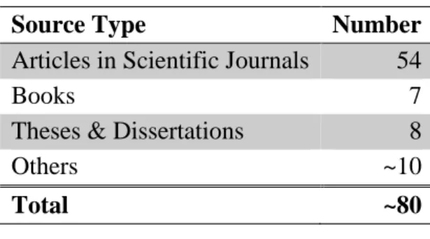
reviewed scientific journals, conference proceedings, books, theses, and dissertations have been scanned and approximately eighty sources are reviewed. A summary of reviewed source types is at Table 1.1. Contents and findings of these reviewed studies will be discussed in Section 2.3.

(17)

Table 1.1 Literature Review, Source Types

Source Type Number

Articles in Scientific Journals 54

Books 7

Theses & Dissertations 8

Others ~10

Total ~80

1.3.2 Software

In every data analysis, a researcher needs some programming tools. For some basic data manipulations Microsoft Excel is used. For the advanced data analytics part of this study, RapidMiner has been extensively used. RapidMiner is a free visual workflow environment where one can use predefined data mining models and develop his/her programming scripts2_.

1.3.3 Data Analysis

Any kind of data analysis project should ideally encompass all or most of the following phases (Tufféry 2011):

1. Identifying the objectives 2. Listing relevant data 3. Collecting the data 4. Exploring the data

5. Preprocessing (blending, cleansing) the data 6. Transforming the data if necessary

7. Training data mining models 8. Tuning model criteria

9. Validating models

(18)

Since the focus of this study is the comparison the data mining models, the objective phase is already included in the project. To be able to compare the findings of this study, publicly available date sets have been chosen and they are already well organized real data. Thus, phases from 2 to 5 can be skipped. Remaining phases comprise the body of this study.

1.4 Outline of the Study

Chapter 2 presents the basics about credit scoring and data mining. Findings of the recent and relevant studies are also given here. Finally date sets used in this study are introduced.

Chapter 3 establishes the foundation of this study. Necessary data transformation steps, aspects of model training and evaluation metrics are clarified.

Chapter 4 presents the experimental setting and gives brief descriptions about data mining models.

(19)

2 BACKGROUND

This chapter introduces the main research topic that is credit scoring and gives a brief introduction to the data mining field. Finally, the data sets are presented and former studies around this subject are evaluated.

2.1 Credit Scoring

After every application for a loan, customers are evaluated by their personal information and historical performance with the aim of estimating their

creditworthiness (Han et al. 2013). This is where credit scoring comes into play. Thanks to the recent developments in cloud technology and big data, there is

tremendous amount of data collected about people. The main aim of credit scoring is to analyze those data and distinguish good payers from bad ones, utilizing

characteristics such as account, purpose of loan, marital status etc. (Mues et al. 2004).

Although no single credit scoring model is perfect and they considerably fail to identify risky borrowers (Finlay 2011), it is the primary tool of lending institutions in making credit decisions. Scoring originally started based on subjective evaluations of experts. Later it was based on 5 Cs: character, capital, collateral, capacity,

conditions. Then, statistical techniques emerged such as linear discriminant analysis, logistic regression. They had been applied successfully for some time, but the problem with those models is they usually require the data not to violate some distributional assumptions such as normality. In recent decades, many studies and applications supported the idea that new data mining techniques such as neural networks, support vector machines can be used as alternatives (Wang et al. 2011). In contrast to statistical methods they do not assume certain distributions. Credit scoring

(20)

2.2 Data Mining

As being an area intertwined with so many disciplines it is argued that data mining is not an actual scientific branch. Rather, it is a set of methods for exploring and

analyzing data sets in an automatic way in order to extract certain unknown or hidden rules, patterns, associations among those data. Data mining has basically two functions: descriptive and predictive. Descriptive techniques are designed to bring out information that is present but buried, while predictive techniques are designed to extrapolate new information based on present information (Tufféry 2011).

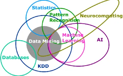
The diagram which is created for a data mining course by experts in SAS Institute back in 1998 demonstrates the complicated nature of data mining field.

Extracting information from data set is an inductive process which means the models learn from the data. There are two common types of learning: unsupervised learning (learning without definite goals), supervised learning (learning with definite goals) (Kantardzic 2011).

Figure 2.1 Data Mining Venn Diagram Source: (Mitchell-Guthrie 1998)

(21)

2.2.1 Unsupervised Learning

Under this learning scheme there is no output or response variable and only the input or explanatory variables are provided to learner. It is expected from the learner to build the model on its own. Since there is no output variable and hence there is no relation to detect, the primary goal of unsupervised learning is to discover natural structure of the data set (Kantardzic 2011). The most common unsupervised learning method is called clustering.

2.2.1.1 Clustering

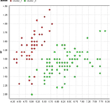
Cluster is a subset of data which are similar out of the whole data set. Clustering is the procedure to categorize each example in a data set into groups such that the members of each group are as similar as possible to one another (Sayad 2016). The chart Figure 2.2 is a demonstration of a clustering learner. The learner assigns every example in the data set to one of the two clusters. There are various models where the number of clusters set beforehand or left to optimization algorithms of learners.

(22)

2.2.2 Supervised Learning

Unlike unsupervised learning, in supervised learning there is definite output variable. The main goal is to reveal the hidden mapping between input variables and the output variable (Brownlee 2016). Most of the data mining tasks fall into this

category. Supervised learning can be further classified into two fields: regression and classification.

2.2.2.1 Regression

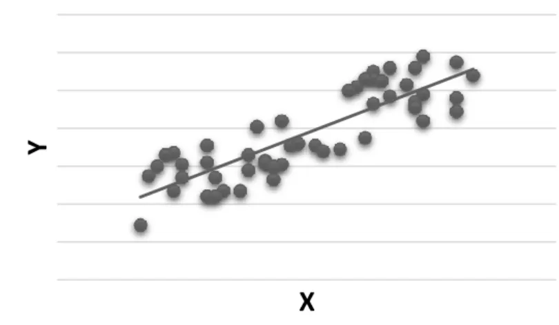
The data mining task becomes regression when the output variable has real values. In very general terms, regression is describing and revealing the relationship between the output variable and one or more input variables. More technically, regression attempts to explain variability in the output variable with respect to movements in the input variables (Brooks 2008). In its simplest form the relationship between output variable and one input variable can be depicted with a linear line as shown in the Figure 2.3

2.2.2.2 Classification

Classification learners are used to reveal the relation between the class of the output variable and input variables. Like clustering learners, classifiers also assign each

Y

X

(23)

example in a data set to a class. The difference is, in classification, classes are already defined. After revealing this relation, learner assigns new examples of which classes are not known to existing classes (Yazdani et al. 2014). Number of classes might be two or more. The special case is having two classes. It is also called binary output variable and this case is also the subject of this study.

In credit scoring the output variable, which is creditworthiness of an entity, takes only one of the values, good or bad. For binary classification tasks, commonly used learners are decision trees, Naïve Bayes, k-nearest neighbor (KNN), artificial neural networks (ANN), support vector machines (SVM), logistic regression, linear

discriminant analysis (LDA), random trees and forests, deep learning. Each of these learners will be performed and their relative successes are evaluated in following sections.

2.3 Former Studies

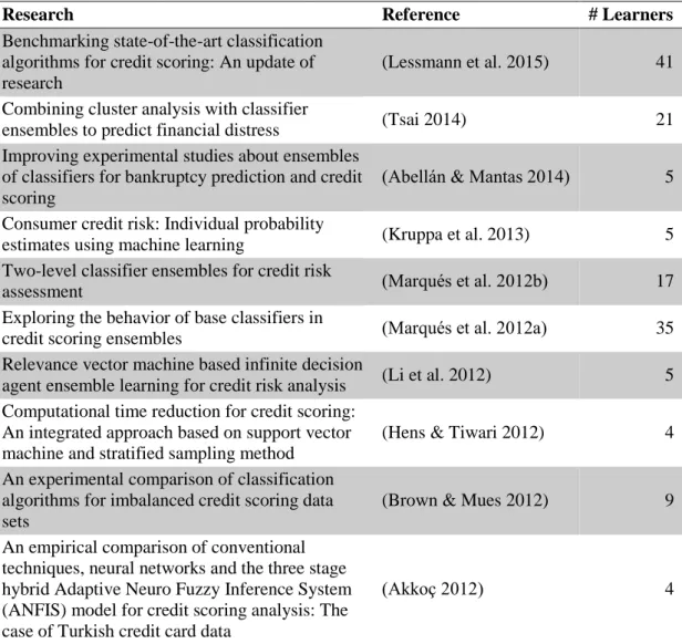
The financial industry utilizing credit scoring systems directly experience the results of their systems, as benefits or losses. Also, because of the central role of the banking industry in the national and the global economy, credit granting policies and systems are highly controlled by local authorities (like BRSA in Turkey) and by BASEL regulations as well. Because of these reasons, the whole industry together with scientists in associated fields try to reach the best model for decades. There are numerous studies only focusing on comparing of statistical and data mining algorithms. A selection of researches in which German and Australian credit data sets has been used is presented at Table 2.1. In addition to this selection, around six studies per year were published in 2010 and 2011 as well.

(24)

Table 2.1 Selection of Researches on Learner Comparison in Credit Scoring

Research Reference # Learners

Benchmarking state-of-the-art classification algorithms for credit scoring: An update of research

(Lessmann et al. 2015) 41 Combining cluster analysis with classifier

ensembles to predict financial distress (Tsai 2014) 21 Improving experimental studies about ensembles

of classifiers for bankruptcy prediction and credit scoring

(Abellán & Mantas 2014) 5 Consumer credit risk: Individual probability

estimates using machine learning (Kruppa et al. 2013) 5 Two-level classifier ensembles for credit risk

assessment (Marqués et al. 2012b) 17

Exploring the behavior of base classifiers in

credit scoring ensembles (Marqués et al. 2012a) 35

Relevance vector machine based infinite decision

agent ensemble learning for credit risk analysis (Li et al. 2012) 5 Computational time reduction for credit scoring:

An integrated approach based on support vector machine and stratified sampling method

(Hens & Tiwari 2012) 4 An experimental comparison of classification

algorithms for imbalanced credit scoring data sets

(Brown & Mues 2012) 9 An empirical comparison of conventional

techniques, neural networks and the three stage hybrid Adaptive Neuro Fuzzy Inference System (ANFIS) model for credit scoring analysis: The case of Turkish credit card data

(Akkoç 2012) 4

Although the data sets are definite and the same across these studies, data transformation steps, such as normalization, applied are numerous, but the underlying rationale is mostly unclear. That is, researchers either assume that the benefit of some data transformation steps are widely known and an explanation is not needed or they apply a specific transformation because the models require so.

Because of these reasons a comprehensive approach is followed in this study and almost every kind of data transformations is applied on the data sets in order to be able to observe the effects of different transformations.

Secondly, in most studies models compared are already limited, that is, they are already shortlisted out of a bigger model set. Yet, the underlying reason behind this

(25)

selection is unclear. That is why a comprehensive approach in model selection is followed also. Each 43 built-in model in RapidMiner is trained on the distinctly transformed data sets and the outcomes are evaluated. The details of these data transformations and model selection are explained in Section 4.1.

Lastly, it is now clear that ensemble models (mostly weighted voting), which

combine single models to increase the overall prediction success, are more successful (Lessmann et al. 2015). However, every ensemble model can possibly include a different combination of single models. The number of choices is practically uncountable. The rationale behind the selection of single models while building the ensemble model is mostly ambiguous among these studies. In other words, there is no objective and definite method which enables practitioners to find the optimum combination of single models to build ensemble model. This is one of the main inquires of this study. If we can find an objective method to select single models than it might be possible to build a totally automated and dynamic system which takes any kind of credit data sets and applies data transformations, tries every model available on them and finally build the most successful ensemble model. Yet, as will be

explained in the final chapter, we failed to find an objective method and the selection of single models to build the most successful ensemble model still requires human interaction.

2.4 Data Exploration

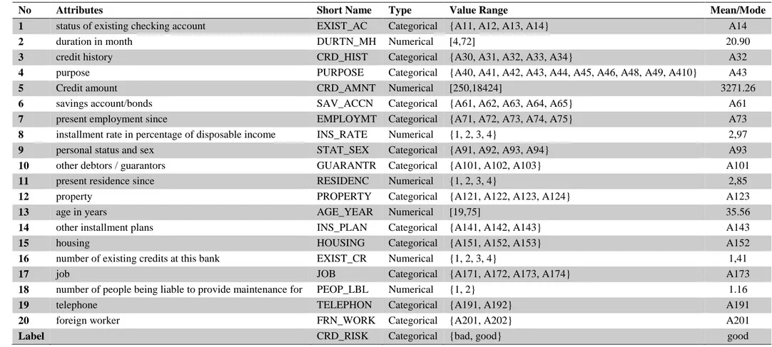
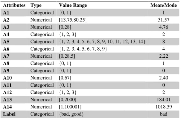
As mentioned before the German credit data set belongs to real loan applicants and Australian credit data set belongs to credit card applications. German data has 1,000 examples and 20 attributes without any missing values. Among 1,000 examples 300 ones are bad credits. So, the ratio of good to bad credits is 7:3 which should not

(26)

attributes, with some missing values. But missing values are replaced by means and modes of corresponding attributes. The ratio of good to bad credits is about 44:56 which is very good. In Australian data set all attributes and values are converted to meaningless symbols to protect privacy. Types of attributes are presented at Table 2.2 and Table 2.3. Detailed description of the data sets and value ranges of attributes are presented at Appendix A: Description of the German credit dataset and Appendix B: Description of the Australian credit dataset.

(27)

Table 2.2 German Credit Data Attributes

No Attributes Short Name Type Value Range Mean/Mode

1 status of existing checking account EXIST_AC Categorical {A11, A12, A13, A14} A14

2 duration in month DURTN_MH Numerical [4,72] 20.90

3 credit history CRD_HIST Categorical {A30, A31, A32, A33, A34} A32

4 purpose PURPOSE Categorical {A40, A41, A42, A43, A44, A45, A46, A48, A49, A410} A43

5 Credit amount CRD_AMNT Numerical [250,18424] 3271.26

6 savings account/bonds SAV_ACCN Categorical {A61, A62, A63, A64, A65} A61

7 present employment since EMPLOYMT Categorical {A71, A72, A73, A74, A75} A73

8 installment rate in percentage of disposable income INS_RATE Numerical {1, 2, 3, 4} 2,97

9 personal status and sex STAT_SEX Categorical {A91, A92, A93, A94} A93

10 other debtors / guarantors GUARANTR Categorical {A101, A102, A103} A101

11 present residence since RESIDENC Numerical {1, 2, 3, 4} 2,85

12 property PROPERTY Categorical {A121, A122, A123, A124} A123

13 age in years AGE_YEAR Numerical [19,75] 35.56

14 other installment plans INS_PLAN Categorical {A141, A142, A143} A143

15 housing HOUSING Categorical {A151, A152, A153} A152

16 number of existing credits at this bank EXIST_CR Numerical {1, 2, 3, 4} 1,41

17 job JOB Categorical {A171, A172, A173, A174} A173

18 number of people being liable to provide maintenance for PEOP_LBL Numerical {1, 2} 1.16

19 telephone TELEPHON Categorical {A191, A192} A191

20 foreign worker FRN_WORK Categorical {A201, A202} A201

(28)

Table 2.3 Australian Credit Data Attributes

Attributes Type Value Range Mean/Mode

A1 Categorical {0, 1} 1 A2 Numerical [13.75,80.25] 31.57 A3 Numerical [0,28] 4.76 A4 Categorical {1, 2, 3} 2 A5 Categorical {1, 2, 3, 4, 5, 6, 7, 8, 9, 10, 11, 12, 13, 14} 8 A6 Categorical {1, 2, 3, 4, 5, 6, 7, 8, 9} 4 A7 Numerical [0,28.5] 2.22 A8 Categorical {0, 1} 1 A9 Categorical {0, 1} 0 A10 Numerical [0,67] 2.40 A11 Categorical {0, 1} 0 A12 Categorical {1, 2, 3} 2 A13 Numerical [0,2000] 184.01 A14 Numerical [1,100001] 1018.39

(29)

3 PREDICTIVE MODELLING

As discussed earlier data mining has basically two functions: description and

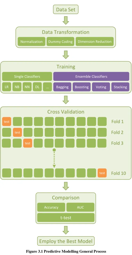
prediction. Describing a data set usually means exploring its statistics, understanding distributional properties etc. Prediction, on the other hand, is related to the future or the unknown rather than what we have at hand. As any kind of data analysis project, predictive modelling, starts firstly with collection of data. After exploring the data if it seems necessary data preprocessing and data transformation is also performed. Afterwards, model is trained until reaching a stable classifier algorithm which can find the hidden pattern in the data set. Then comes validating the findings of the model with the facts. After successful completion of the validation step a model becomes ready to deploy, that is, to predict (Imanuel 2016). The structure of the overall predictive modelling is illustrated in Figure 3.1.

(30)

Data Transformation

Normalization Dummy Coding Dimension Reduction

Training

Ensemble Classifiers

Bagging Boosting Voting Stacking Single Classifiers LR NB NN DL …

Data Set

Comparison

Accuracy AUC

t-test

Cross Validation

test test test test

Fold 1

Fold 10

Fold 2

Fold 3

Employ the Best Model

(31)

3.1 Data Transformation

Transforming the data is often performed to improve the capabilities of data mining models in finding the patterns. The type of transformation required depends on the learning method (unsupervised, supervised etc.) and the data itself (Baesens et al. 2009). Major data transformation methods are missing value imputation,

normalization, discretization (binning, coarse categorization), dummy coding, and dimension reduction.

3.1.1 Missing Value Imputation

If there are some attributes in the data set which have missing values, this should be dealt first since models will fail to extract information from those examples. The simplest method would be taking out the attribute with missing values entirely. However, removal of an entire attribute together with its examples which carry information causes the learning process to be incomplete and biased. Instead of removing, missing values can be replaced with pseudo values in order to provide the learning algorithm with a full data set without any loss of information. The first method would be replacing missing values with the averages (or medians/modes depending on the data) of corresponding attributes. This method brings some

benefits, but it is very risky also. If the number of missing values are relatively high, then replacement with average values can change the whole distribution of the attribute values and causes the algorithms to learn a different data set than the real one. Thus, less risky and precise methods are needed (Tufféry 2011).

Remedy for this is replacing missing values with statistical approaches and it is called missing value imputation. Depending on the type of the data, there are a couple of accepted techniques to follow. Discussion of these techniques are beyond

(32)

this study. Throughout this study whenever it necessary imputation of missing values will be conducted with KNN model as the most widespread statistical solution.

3.1.2 Normalization

Some data mining methods, especially those that are based on the distance computation between examples in n-dimension need normalized data in order to diminish the effects of extreme values and handle different attributes at similar scale. Among normalization methods most widely used one is the normalization based on standard normal distribution, also called standardization. In this method, each value of an attribute is converted according to the equation 3.1, where 𝑋̅ is the average of the values of an attribute and 𝑆_𝑋 is the standard deviation of those values.

𝑁𝑖 =

𝑋𝑖− 𝑋̅ 𝑆𝑋

(3.1)

After the conversion, the distributions of numerical attributes become similar to normal distribution, thus can be efficiently used by data mining methods which require normality assumptions.

3.1.3 Discretization

When the values of an attribute are in continuous numerical form, sometimes there are benefits of categorizing (binning) those values into finite set of values before the learning process. Though at first it seems losing information, discretization is

especially useful in three cases. When missing values exist in the data set and imputation is conducted, it is a tricky situation. Imputation might impair the distribution of the true population. However, through discretization missing values can be categorized into a distinct set and evaluated accordingly. Second, the

(33)

an extreme age value 110 may distort especially regression models. Instead of using this extreme value as it is, categorizing age values and putting this 110 into

“>65 years old” class may solve the problem. Why 65? It comes from the domain knowledge of credit decision. Since the common retirement age is around 65 in most countries there is no harm in assuming that retired customers behave similarly and categorizing them into the same group. Finally, discretization improves the

robustness of logistic regressions by reducing the possibility of overfitting (Tufféry 2011).

The crucial aspect of discretization is the final number of categories and the cut-off points of these categories. In the literature, three to six final categories are

recommended (Mctiernan 2016). Cut-off points can be determined by domain knowledge as in the example above, or by fixing the number of categories, or by distributing the number of values evenly into the categories. Instead of choosing cut-off points, categories can be determined by automatic procedures. For instance, in this study discretization by entropy approach is followed where cut-off points are set so that the entropy is minimized in the categories. After applying this technique, the distribution of CRD_AMNT attribute has changed as shown in the Figure 3.2. The cut-off point 3913 has been automatically chosen which minimizes entropy of classes.

(34)

3.1.4 Dummy Coding

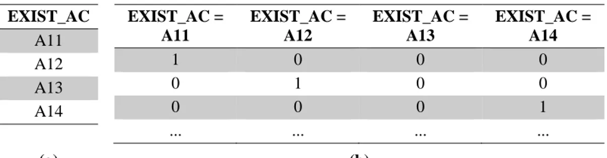
Some data mining methods like neural networks and support vector machines require the data set to fully in numerical form. In order to utilize these models categorical (nominal) values are converted to numerical values in dummy coding. In this coding style, for every existing value of a categorical variable a new binary attribute is created and take the values of 0 or 1. For instance, in German credit data set,

EXIST_AC attribute normally has the values in Table 3.1.a and for each value of this variable new attributes are created in Table 3.1.b.

Table 3.1 Conversion of Categorical to Numerical Values EXIST_AC A11 A12 A13 A14 EXIST_AC = A11 EXIST_AC = A12 EXIST_AC = A13 EXIST_AC = A14 1 0 0 0 0 1 0 0 0 0 0 1 ... ... ... ... (a) (b)

(35)

3.1.5 Dimension Reduction

As will be discussed further in the study two of the most successful and widespread data mining methods in credit scoring are logistic regression and support vector machine. Both suffer from high number of dimensions of the data set. The higher the number of attributes in a data set the more possible the model suffers from

multicollinearity. Also it will take so much more time for the model to learn (Han et al. 2013). To decrease the number of attributes in a data set two basic approaches can be followed: principal component analysis and stepwise feature selection.

3.1.5.1 Principal Component Analysis (PCA)

The basic idea of PCA is to reduce the dimension number of a data set where there are large number of interrelated variables, while preserving as much as possible of the variation. This reduction is achieved through creation of new attributes from existing ones, which are uncorrelated, independent and ordered in terms of their explanatory power (Tsai 2009). In this study, when PCA is conducted new attributes are kept as long as their total variance is under 0.95. That is, any attribute which explains so little variability in the target attribute excluded from the model.

3.1.5.2 Stepwise Feature Selection

In stepwise feature selection, there are basically two directions along which the selection process can be conducted: forward or backward. Backward selection (elimination) procedure starts with the most complex model, which is including all explanatory attributes. After learning the most complex model and logging its performance measure, remaining attributes are excluded from the learning procedure one by one. The performance of the model which has less explanatory variables is tested against the model which has more explanatory variables through F-test. If

(36)

performance than those attributes are kept out of the model. Until there is no significant improvement this procedure continues where the model has minimum number of attributes eventually.

Forward selection is exactly the opposite of the backward selection. Attributes are added to the simplest model and larger models are tested against more simple ones. The number of attributes (20) of the data set of this study is relatively high, thus, forward selection will be much more time consuming. Thereby, during feature selection phase backward elimination approach will be followed.

3.2 Training

After exploring and making necessary transformations the data set becomes ready to be used in the training phase. In this phase a sample of examples is drawn from the population whose target values are known. The model tries to extract the hidden pattern between the target feature and the explanatory variables in this phase. After reaching a pattern the model is tested on a sample of examples unseen before whose target values are also known (Tufféry 2011). If the test results are promising the model may be deployed on new data to predict its target value.

The main objective of the training procedure is not only to extract the pattern between output and input variables but also to produce generalizable models which can be performed on new unseen data for predicting purposes. In some cases, especially when the size of the training set is small and the complexity of the model is high, the model might capture the exact representation of this small training set and perfectly predict target values, but it might fail to correctly predict the target values of unseen examples. This phenomenon is one of the fundamental problems of model training and is called overfitting (Giudici & Figini 2009).

(37)

3.2.1 Overfitting Problem

In other words, overfitting occurs when the model memorizes the pattern between the output and input variables even though this pattern does not exist in the whole

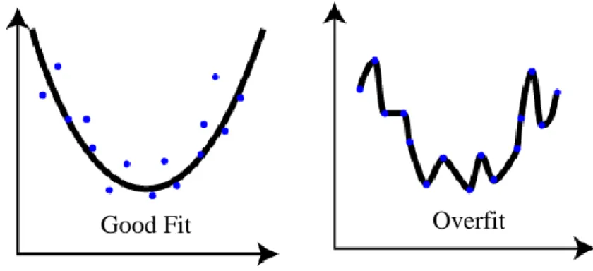
population. Overfitting usually happens when the training data set is small and is especially observed with models decision trees and neural networks. When it happens the model typically fits to the examples too perfectly. It can easily be revealed by testing the model on unseen data. If there is significant discrepancy between the error rate of the training set and test set there is probably overfitting (Tufféry 2011). Graphical representation of an overfitting model can be observed at Figure 3.3. As can be seen, the right model perfectly fits to the training (existing) examples but it loses the ability to generalize. However, the left model has larger errors but it generalizes well. New unseen points will be closer to the left model.

Another aspect of overfitting is error rate which corresponds to the complexity of the model in addition to the training size. In data mining, bias means error rate on the training data set and variance denotes how dispersed the model results on the test set. The more complex the model, i.e. the more perfectly it fits, the less bias it will have at the expense of losing generalizability because of the high variance. There is an optimal point where the model has acceptable bias and variance. Figure 3.4

Good Fit Overfit

(38)

true optimal point is hard to find there is a way to validate the generalizability of the model called cross validation (CV) or more specifically k-fold cross validation.

3.2.2 K-fold Cross Validation (CV)

As discussed in the previous part measuring only the error rate on the training set is not conclusive to estimate true model performance. What is required is to be able to measure the total error rate of the model. To achieve this the error rate of the model must be measured on new, unseen data, ideally more than once (Seni & Elder 2010). This is where cross-validation comes into play. “Cross-Validation is a statistical method of evaluating and comparing learning algorithms by dividing data into two segments: one used to learn or train a model and the other used to validate the model.” (Refaeilzadeh et al. 2009).

K-fold cross validation is a special form of cross-validation where the whole data set is divided into k nonoverlapping parts (folds). Each of these k parts is used as test set while remaining k-1 sets are used for training. Therefore, every learnt model will be

Figure 3.4 Bias-Variance Trade-Off

(39)

tested on a different test. After performing training and testing k times the model is evaluated by the average error rate (or performance). The graphical representation of this procedure is illustrated in Figure 3.1. In the cross-validation rectangle each row (ten squares) represents the overall data set and corresponding one training and testing phase. Each orange square is left out as test set and remaining nine green squares are used as one whole training set. This process is iteratively repeated k times. In literature, k is usually set to 10. In this study this custom will be followed and whenever k-fold cross validation is performed it means 10-fold CV.

Validation of predictive capabilities of a data mining model obviously requires standard measurement units. In the next part, performance measures that are used in the evaluation and comparisons of the models will be briefly explained.

3.3 Measures of Performance

In binary problems, models use mathematical functions to map input variables to one of the two classes of the output variable. Most of the time, models’ functions assign numerical values to examples possible to order and rank. These numerical outcomes are called confidence. They are basically probabilistic assessments and take values within the range [0,1]. Depending on the business strategy a threshold or cut-off point is chosen and examples are classified according to this threshold. Most of the time, 0.5 is chosen as threshold value. Mathematically,

𝑖𝑓 𝐶𝑜𝑛𝑓𝑖𝑑𝑒𝑛𝑐𝑒𝑖 (𝑐𝑖) > 𝑇ℎ𝑟𝑒𝑠ℎ𝑜𝑙𝑑 (𝜃) , 𝑎𝑠𝑠𝑖𝑔𝑛 𝑝𝑜𝑠𝑖𝑡𝑖𝑣𝑒 𝑐𝑙𝑎𝑠s (3.2) 𝑖𝑓 𝐶𝑜𝑛𝑓𝑖𝑑𝑒𝑛𝑐𝑒𝑖 (𝑐𝑖) ≤ 𝑇ℎ𝑟𝑒𝑠ℎ𝑜𝑙𝑑 (𝜃) , 𝑎𝑠𝑠𝑖𝑔𝑛 𝑛𝑒𝑔𝑎𝑡𝑖𝑣𝑒 𝑐𝑙𝑎𝑠s (3.3)

(40)

In the end, each example in the data set has both an actual class value and a predicted class value. The distribution of these values is represented in a two-by-two

contingency table called confusion matrix.

3.3.1 Confusion Matrix

The number of examples classified by a binary classification algorithm can be depicted as in the Table 3.2. In credit scoring terminology, positive values denote bad credits (defaults), while negative values denote good credits (healthy). That bad credits take the value positive may seem counter intuitive at first, yet ‘positive’ signifies the focus of the data mining problem at hand.

Table 3.2 Confusion Matrix

Actual Classes Good Credit Bad Credit

Predicted Classes

Good Credit True Negatives (TN)

False Negatives (FN) Bad Credit False Positives

(FP)

True Positives (TP)

From this table a couple of metrics can be calculated each of which conveys distinct meaning with respect to the success of the model. Most widely used accuracy metrics are calculated as follows.

𝑆𝑒𝑛𝑠𝑖𝑡𝑖𝑣𝑖𝑡𝑦 = 𝑅𝑒𝑐𝑎𝑙𝑙 = 𝑇𝑟𝑢𝑒 𝑃𝑜𝑠𝑖𝑡𝑖𝑣𝑒 𝑅𝑎𝑡𝑒 = 𝑇𝑃𝑅 = 𝑇𝑃 𝐹𝑁 + 𝑇𝑃 (3.4) 𝑆𝑝𝑒𝑐𝑖𝑓𝑖𝑐𝑖𝑡𝑦 = 𝑇𝑟𝑢𝑒 𝑁𝑒𝑔𝑎𝑡𝑖𝑣𝑒 𝑅𝑎𝑡𝑒 = 𝑇𝑁𝑅 = 𝑇𝑁 𝑇𝑁 + 𝐹𝑃 (3.5) 𝐹𝑎𝑙𝑠𝑒 𝑃𝑜𝑠𝑖𝑡𝑖𝑣𝑒 𝑅𝑎𝑡𝑒 = 𝐹𝑃𝑅 = 𝐹𝑃 𝑇𝑁 + 𝐹𝑃= 1 − 𝑆𝑝𝑒𝑐𝑖𝑓𝑖𝑡y (3.6) 𝐴𝑐𝑐𝑢𝑟𝑎𝑐𝑦 = 𝑇𝑃 + 𝑇𝑁 𝑇𝑁 + 𝐹𝑁 + 𝐹𝑃 + 𝑇𝑃= 𝑇𝑃 + 𝑇𝑁 𝑇𝑜𝑡𝑎𝑙 (3.7)

(41)

Sensitivity measures the proportion of positive examples, bad credits in credit scoring that are correctly identified. In credit scoring terms, this is the proportion of defaulted persons that are detected by the model. Specificity measures the proportion of negative cases that are correctly identified. In credit scoring terms, these are the examples of good credits correctly classified by the model. False positive rate represents the proportion of examples that are classified as default incorrectly. In statistical terms, it is called Type I error. Finally, accuracy measures the overall success of the model. It is the proportion of correctly classified cases, either default or not, to total cases.

3.3.2 Accuracy, ROC & AUC

Although accuracy measurement demonstrates how successful a model is in binary classification, the resultant distribution tabulated in the confusion matrix depends on the threshold chosen in the first place. Intuitively, 𝜃 is fixed at 0.5. But, strategically the selection of the threshold value depends on the cost misclassified cases bring about. For instance, in credit scoring scheme granting credit to a bad borrower (false negative) is worse than rejecting an applicant who is actually a good borrower (false positive). Therefore, threshold selection is very crucial and the effect of this selection on the overall accuracy of the model must be observed.

Mathematically, threshold value can be anything in the range (0,1). Hence, the number of the distributions of different classifications is practically uncountable. There exists a graphical tool which solves this problem which is called receiver operating characteristic (ROC). The name comes from the field where this tool is first created. In data mining, ROC acronym has widespread usage. ROC graph is basically a collection of success rates of a model for every possible threshold values.

(42)

rate (1-specificity). A typical ROC graph can be observed in the Figure 3.5. The perfect model flawlessly discriminates two classes. For instance, (0,1) point means the model catches all defaults while making no mistake in healthy examples as well. Random model has no discriminatory power at all. The model outcomes in between the perfect and random model discriminate at varying degrees depending on the threshold value. Along the ROC curve every possible success rate couples are shown for every threshold values (Khudnitskaya 2010).

The nearer a ROC curve to the upper left corner the more successful it is in

discriminating classes. Since visual comparison does not provide conclusive result, we need scalar accuracy values to compare. The solution for that is calculating the area under the ROC curve. It is called AUC and is probably most widely used performance metric in binary classification problems. AUC will be primary

False Positive Rate (1-Specificity)

Tru e P o sit iv e Ra te (S en siti vity ) Random Model

(43)

measurement metric throughout this study also. AUC value makes class distribution based on different threshold values irrelevant. Since the ROC graph is drawn on a unit square the area under the hypothetical perfect model sums up to 1. The area under the random model is 0.5. Therefore, it is expected from any binary

classification model to have at least 0.5 AUC and as closer as possible to 1 (Kraus 2014).

3.3.3 Pairwise T-Testing

In order to evaluate performance outcomes of different models an accurate

comparison system is also required. Because, one model outcome does not represent its true population mean and several trials will yield different results while

converging the true performance of the model. So, if one performance outcome of a model is compared to another one the assessment might be wrong. To compare model outcomes consistently, t-test will be applied on AUC values. T-test is a statistical comparison technique which allows to test whether two groups of values comes from the same population. In other words, in credit scoring performance, t-test will allow us to distinguish only significantly successful data mining models.

(44)

4 EXPERIMENTATION

The process of the experimentation involves four phases: making necessary data transformations to improve model accuracies, setting the software environment to let the models learn on the training data and logging the performance results, comparing the models to each other, and finally building the ensemble model. To complete the first three phases efficiently a reproducible program is created, which can handle almost any kind of data and make necessary transformations, called model comparison engine (MCE).

4.1 Model Comparison Engine

As discussed in the latest chapter in most cases data needs to be cleansed and transformed in order the models to fully utilize it. In this study, since some models require the data to be in numerical/categorical form and some has comparative advantages on some data types and we wanted to create an exhaustive comparison universe where each model will be able to have all necessary conditions to reach its true potential and to maximize its performance results.

The first part of MCE checks the properties of the data set. If the data set has missing values in it, those missing values are replaced by missing value imputation technique described in section 3.1.1. However, at the end of this step the original data set which has missing values is not thrown away, rather two data sets are kept: (1) with missing values, (2) without missing values. The main reason to keep the original data set with missing values is to give the opportunity to the models which can handle missing values.

Since there are models based on the distance between data points, like support vector machines which try to find optimal lines or surfaces which divides the data set in the

(45)

n-dimensional space, the scale of the numerical data, thus, normalization is also important. In the second step, all numerical values are normalized by the method explained in the section 3.1.2. Again, the data set which has nonnormalized numerical attributes is not neglected, it will be kept together with normalized data set. Until now, if the data set has required missing value imputation also, we will now have four different data sets. This is the central idea of model comparison engine.

The next step is to create discrete categories out of numerical values. The underlying reason, method and possible benefits of discretization has been discussed in section 3.1.3. After completing discretization, all categorical variables are converted to numerical variable in dummy coding form described in section 3.1.4. As a last step dimension reduction is performed on all the attributes, without making any

distinction between attributes which exist in the original data set and attributes created afterwards.

There are some steps which need more clarification. As discussed before, some models like support vector machines and neural networks require data set to be in numerical form. This was the main reason of dummy coding. Yet the sequential application of data transformations causes some meaningless data sets to emerge. For instance, a data set which is already in numerical form can be discretized and codded in dummy form afterwards. This obviously will cause data loss. Since designing the algorithm in RapidMiner accordingly is costly, all kinds of transformations applied regardless of their logical base. Corresponding results have less accuracy and therefore do no impair the general evaluation of the study.

(46)

After the data transformation is completed we might have 64 or less distinct data sets depending on the properties of the initial data set. Figure 4.1 illustrates the data transformation steps and illuminates in visual representation how the number of data sets increase exponentially. In this figure each rectangle represents a distinct data set from which models try to extract hidden pattern.

The resultant data sets of this transformation phase are fed to the learning algorithms. Similar to the transformation steps, in this study we wanted to try as many models as possible on every distinct data sets. To this end, learning algorithms of almost any kind are listed and grouped under classifier families. Since detailed descriptions and explanation of underlying mapping functions of these models are beyond the scope of this study, larger classifier families will be explained briefly.

o

riginal

da

ta

no transformation no transformation no transformation discretization normalization normalization normalization + discretization imputation imputation imputation imputation + discretization imputation + normalization imputation + normalization imputation + normalization + discretization 64 8 4 2 1

(47)

4.2 Classifier Families

As discussed earlier in this study for data analytics purposes RapidMiner is used as software. RapidMiner has 43 built-in single models ready to deploy with default parameters. Each of this model is included in model comparison engine with default settings and grouped under a classifier family. Models and their corresponding classifier families are listed in Table 4.1.

(48)

Table 4.1 RapidMiner Classifier Families & Models

No Classifier Families Model Name 1 Functions (Regressions) Gaussian Process

2 Generalized Linear Model

3 Linear Regression

4 Local Polynomial Regression

5 Polynomial Regression

6 Relevance Vector Machine

7 Seemingly Unrelated Regression

8 Vector Linear Regression

9 Support Vector Machines Fast Large Margin

10 Hyper Hyper

11 Support Vector Machine

12 Support Vector Machine (Evolutionary)

13 Support Vector Machine (LibSVM)

14 Support Vector Machine (Linear)

15 Support Vector Machine (PSO)

16 Logistic Regressions Logistic Regression

17 Logistic Regression (Evolutionary)

18 Logistic Regression (SVM)

19 Bayesian Classifiers Naive Bayes

20 Naive Bayes (Kernel)

21 Decision Trees CHAID

22 Decision Stump

23 Decision Tree

24 Decision Tree (Multiway)

25 Decision Tree (Weight-Based)

26 Gradient Boosted Trees

27 ID3

28 Random Forest

29 Random Tree

30 Neural Networks AutoMLP

31 Deep Learning

32 Neural Net

33 Perceptron

34 Discriminant Analysis Linear Discriminant Analysis

35 Quadratic Discriminant Analysis

36 Regularized Discriminant Analysis

37 Lazy Default Model

38 k-NN

39 Rules Rule Induction

40 Single Rule Induction

41 Single Rule Induction (Single Attribute)

42 Subgroup Discovery

(49)

So far, if each data transformation step is performed then there might be 64 distinct data sets. As the main strategy is trying as many data-model pairings as possible, each of these 64 data sets will be fed to each single model listed. Model comparison engine will try 2752 (43 ∗ 64) possible pairings during this phase and let the models learn the underlying pattern. The overall procedure lasts 20 minutes to 10 hours depending on the number of dimensions, number of examples and complexities of the models applicable. If the pairing causes an error, for instance when categorical variables are fed to support vector machine, MCE will log this error and pass the next trial. In the end, the performance values of every pairings which do not have any error will be logged and saved for comparison. In the coming parts, important

classifier families will be briefly explained.

4.2.1 Functions (Regressions)

Data mining methods which belong to function or regression family were briefly reviewed in section 2.2.2.1. Regressions are basically used to relate output variable to input variables through a mathematical equation. This equation not only helps to predict target values of new input variables but also provides an understanding about the nature of the relationship between output and input variables. In its simplest form regression equation is linear and hence called linear regression. The equation below is a simple example of a linear regression.

𝑌 = 𝛽0+ ∑ 𝛽𝑖∗ 𝑋𝑖+ 𝜀𝑖 (4.1)

Here, 𝑋𝑖 denotes the matrix of input variables, 𝛽𝑖 denotes vector of coefficients for input variables, 𝛽0 denotes constant coefficient and 𝜀𝑖 denotes error term. 𝛽0 and 𝛽𝑖 are calculated through an optimization method called ordinary least squares which minimizes the sum of

(50)

squared errors. Figure 2.1 depicts the line of this equation in its simplest form where there is only one input variable.

4.2.2 Support Vector Machines (SVM)

Compared to the other data mining classification methods, support vector machines (SVM) are newly developed in the nineties by Vladimir Vapnik. SVM is especially useful on linearly separable examples. When, however, data points are clustered in n-dimensional space there might be infinite number of linear boundaries which separate those clusters. What SVM does essentially is to find the optimal hyperplane that maximizes the width of the margin between observation clusters (Tufféry 2011). Figure 4.2 shows how the optimal hyperplane separates different classes by widest possible margin.

There are a couple of advantages of using SVM over other data mining algorithms. First, training process is comparatively easy with even small number of parameters and the final model is not presented with a local optimum, unlike some other techniques. Second, SVM scales to high dimensional data relatively well. Some of the recent and most successful applications of SVM have been in image processing,

Figure 4.2 Support Vector Machine Hyperplane

(51)

particularly hand written letter recognition and face recognition (Kantardzic 2011). One of the aspects of SVM which is often criticized is its opaque methodology (Harris 2015).

4.2.3 Logistic Regressions

As one of the oldest classification methods in statistics, logistic regression is the most widely used classification technique in credit scoring (Huang & Day 2013). Its popularity is not without reason. It can handle dependent variable with two or more values and independent variables could be numerical or categorical. The results of logistic regression are clear and interpretable, that is, results have practical meaning especially in credit scoring as probability of default. Finally, logistic regression is one of the most reliable classification methods (Tufféry 2011).

Within the context of credit scoring the aim of using logistic regression is to detect whether counterparties (whether real people or companies) will pay their debts in time. The event of nonpayment or (depending on the problem setting) restructuring of the debt is denoted by positive (bad) class. Whereas, the event where everything goes normal and the borrower pays the debt promptly is denoted by negative (good) class. The fundamental equations of logistic regression are as follows:

Pr(𝑌 = "𝑏𝑎𝑑"|𝑋) = 𝑒 𝛽0+∑ 𝛽𝑖 𝑖∗𝑋𝑖 1 + 𝑒𝛽0+∑ 𝛽𝑖 𝑖∗𝑋𝑖 (4.2) Pr(𝑌 = "𝑔𝑜𝑜𝑑"|𝑋) = 1 1 + 𝑒𝛽0+∑ 𝛽𝑖 𝑖∗𝑋𝑖 (4.3)

In the first equation, what the logistic regression model produces the conditional probability of a nonpayment, given that some explanatory variables exist and their

(52)

representation of a logistic regression equation, where the value logit (𝐿) along the horizontal axis is calculated by a linear equation of 𝑋 values, 𝐿 = 𝛽₀+ ∑ 𝛽_𝑖 _𝑖∗ 𝑋_𝑖. If the logit value is used in the fundamental equation instead of 𝑋 values, the main equation becomes

Pr(𝑌 = "𝑏𝑎𝑑"|𝑋) = 𝑒 𝐿

1 + 𝑒𝐿 (4.4)

4.2.4 Bayesian Classifiers

Bayesian classification method is also one of the simplest and most widely used probabilistic learning methods. What it learns from the training data is the

conditional probability of each attribute 𝐴_𝑖 where the class label 𝐶 is known. The strong major assumption is that all attributes are independent. The assumption of conditional independence of variable is very crucial in order for this method to produce robust results (Twala 2010).

𝑃𝑟(𝑌 = "𝑏𝑎𝑑"|𝑋) = 𝑒

𝛽0+∑ 𝛽𝑖 𝑖∗𝑋𝑖

1 + 𝑒𝛽0+∑ 𝛽𝑖 𝑖∗𝑋𝑖

(53)

4.2.5 Decision Trees

Decision trees are arguably the most intuitive and popular data mining method among others. It provides explicit and easy rules for classification. These rules are easy both to implement on new examples and to present the findings to third parties. Decision trees handle some of the challenging problems of data mining very well also. It can operate on heterogeneous data. It is not affected by missing values and also non-linearity of input variables because it does not rely on the distributional assumptions (Tufféry 2011).

Despite its easiness and popularity decision trees produce relatively poorer results than other data mining methods in credit scoring. This is mainly because of two reasons: (1) The noise and (2) the redundant variables in the data affect the performance of decision trees (Wang et al. 2012).

Decision trees, as the name suggests, a tree-like top-down structure which has root, nodes, branches, and leaves. Each internal node represents a test on one attribute and each branch denotes the outcome of this test. The leaves (terminal nodes) represents either a pure class or a class distribution. The top node in the tree is the root node with the highest information gain. After the root node, among the remaining attributes the one with the highest information gain is chosen and test is performed on this node. The overall process continues until there is no remaining attribute on which example set can be partitioned (Tsai et al. 2014). A decision tree algorithm performed on the German credit data set is presented in Figure 4.4.

(54)

4.3 Ensemble Models

Ensemble models combine single models into a model which is hoped to be more successful than its constituent models. The idea is that every model does not have the same error for a specific example (observation, data point) and they complement each other. Ensemble models have gained widespread usage since they are deemed the most profound development in data mining field in the last decade (Seni & Elder 2010). Especially in credit scoring, where the predictive capability is more important than interpretability of the model, ensemble models provide significant gains over single models’ prediction accuracies.

Ensemble models can be categorized into two broader classes: homogeneous ensemble classifiers and heterogeneous ensemble classifiers. Homogeneous

ensemble classifiers combine the outcomes of the same base model. One of the most widely used such classifiers is bagging (bootstrap aggregating) where independent

(55)

small samples is drawn from the whole data set with replacement and the base model is trained on each one of them. In the end, bagging method combines all predictions. Unlike bagging, in boosting algorithm, constituent models depend on each other. Every next iteration of the boosted algorithm learns from the mistakes of the previous one.

Heterogeneous ensemble classifiers combine multiple different single models to create the final more successful model. Basically there are two heterogeneous models: stacking and voting. In stacking method outcomes of each base models are collected and together with existing examples (instances) a new data set is created. Usually logistic regression with regularization is learnt on this final data set. In voting scheme, the outcomes of single models for every example are compared and the final decision is made either by majority voting or weighted voting (Wang et al. 2011). The most recent studies which compare accuracies of different ensemble models point to the weighted voting as the most successful ensemble model (Lessmann et al. 2015). In order to keep the focus of the study on finding the most successful models automatically and dynamically, ensemble models other than weighted voting have not been employed in this study.

4.4 Weighted Voting

In binary classification problems, the first outcome of the models is the confidence value which shows how confident the model is in predicting the class of an example. In credit scoring this confidence value is usually interpreted as the probability of default of the examined entity. In other words, the confidence value indicates how likely the counterparty fails to pay its debt on time. Weighted voting ensemble model takes the average of the class predictions of single models using their confidence