ISTANBUL BILGI UNIVERSITY INSTITUTE OF SOCIAL SCIENCES
FINANCIAL ECONOMICS MASTER'S DEGREE PROGRAM
THE RELATIONSHIP BETWEEN CREDIT AMOUNT OF SMES AND ECONOMIC GROWTH
Yunus Ertuğrul BAL 115664009
Assoc. Prof. Dr. Serda Selin ÖZTÜRK
İSTANBUL 2017
ACKNOWLEDGEMENTS
I would like to thank Assoc. Prof. Dr. Serda Selin Öztürk, my dissertation advisor, for her guidance, support and patience that she has shown me throughout all stages of my dissertation. My special thanks to Dr. Melik ERTUĞRUL for his kind guidance, invaluable comments, feedbacks and advice. I am sincerely and utterly grateful to my mother, father and sister for their continuous support.
iv CONTENTS
INTRODUCTION ... 1
1 OVERVIEW OF SME, BANK CREDITS, ECONOMIC GROWTH AND FINANCIAL SECTOR DEVELOPMENT ... 3
1.1 SMEs ... 3
1.1.1 Definition of SMEs ... 3
1.1.2 Characteristics of SMEs in General ... 3
1.1.3 Characteristics of SMEs in Turkey ... 4
1.1.4 Importance of SMEs ... 5
1.1.5 Disadvantages of SMEs ... 6
1.2 Bank Credits ... 6
1.2.1 Definition of Credit... 6
1.2.2 Functions of Credits ... 7
1.2.3 Economic and Financial Effects of Bank Credits ... 8
1.3 Economic Growth ... 11
1.3.1 Definition of Economic Growth ... 11
1.3.2 Factors of Economic Growth ... 12
1.3.3 Calculating of Economic Growth ... 15
1.4 Financial Sector Development ... 16
1.4.1 Financial System Functions ... 17
2 REVIEW OF LITERATURE ... 19
2.1 The Relationship between Credit Amount of SMEs and Economic Growth ... 19
2.1.1 Brief Introduction ... 19
2.1.2 Literature Survey ... 20
3 DATA AND METHODOLOGY ... 23
3.1 Definitions of Data and Scope ... 23
3.1.1 Data for SME Loans ... 23
3.1.2 Data for Economic Growth... 23
3.1.3 Methodology ... 23
4 EMPIRICAL STUDY ... 38
4.1 Data Analysis ... 38
4.2 Augmented Dickey Fuller Unit Root Test ... 39
v
4.4 VAR ... 42
4.5 Granger Causality Test ... 45
CONCLUCISION ... 47
vi ABBREVIATIONS
ADF: Augmented Dickey Fuller AIC: Akaike Information Criterion
BRSA: Banking Regulation and Supervision Agency (Bankacılık Düzenleme ve Denetleme Kuruluşu - BDDK)
DSP: Difference-Stationary GDP: Gross Domestic Product GNP: Gross National Product
HQ: Hannan-Quinn Information Criterion IR: Impulse-Response
OECD: Organiztion for Economic Cooperation and Development SIC: Schwartz Information Criterion
SME: Small and Medium Enterpraise TSP: Trend-Stationary
TURKSTAT: Turkish Statistical Institute (Türkiye İstatistik Kurumu - TÜİK) VAR: Vector Auto Regression
vii LIST OF FIGURES
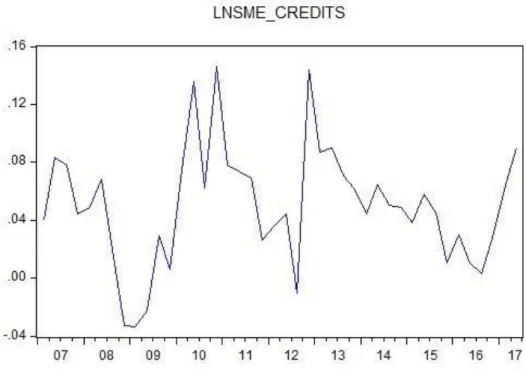
Figure 4.1: Graph of SME Credits ... 38
Figure 4.2: Graph of GDP ... 39
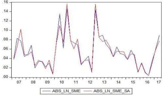
Figure 4.3: Graph of Seasonality Adjusted SME Credits with SME Credits ... 41
Figure 4.4: Graph of Seasonality Adjusted GDP with GDP ... 41
viii LIST OF TABLES
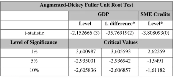
Table 4.1: Results of Augmented Dickey Fuller Test Results ... 40
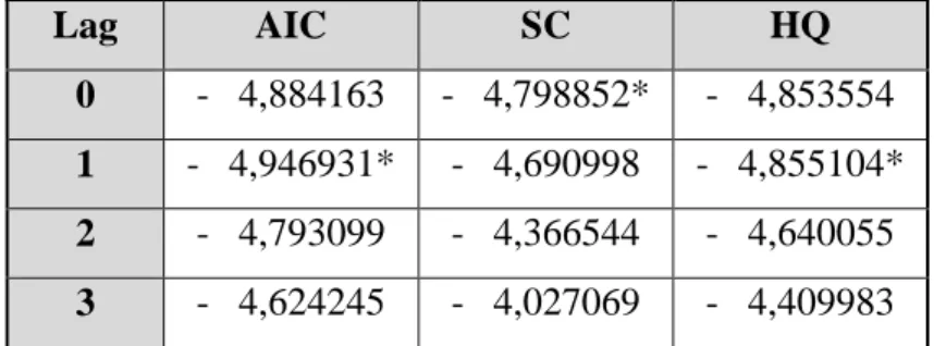
Table 4.2: AIC, SIC, HQ İnformation Criterion ... 42
Table 4.3: Variance Decomposition of SME Credits and GDP ... 44
ix ABSTRACT
Economic growth is one of the most significant indicators of the progress of a country's economy as monetary and fiscal policies are determined in line with the level of economic growth. Countries eventually try to maximize their
economies. Efficient use of resources is one of the most critical subject of
economic growth. Banks credits which generate a large part of financial resources in developing countries have a role in terms of economic growth. Companies, which are among the key dynamics of the economy, use bank credits to increase their output and contribute to economic growth. Companies are divided into several categories based on certain criteria. Small and medium-sized enterprises are one of these classes. The credits that has given to SMEs are one of the main elements of the study with economic growth rate.
This study examines the causality relationship between economic growth and the amount of SME credits by using quarterly annual data from 2007: 1 to 2017: 2. First, the stationarity test has applied to the time series. Secondly, VAR analysis has performed in the aim of working afterwards, impulse-response functions, variance decomposition and lastly Granger causality test have applied to series.
As a result, there was no causal relationship between the amount of credit used and the economic growth in the period of the crisis.
Key words
Economic Growth, SME Credits, Stationarity, VAR, Impulse-Response, Variance Decomposition, Causality
x ÖZET
Ekonomik büyüme bir ülke ekonomisinin gidişatı hakkında bilgi veren önemli göstergelerden birisidir. Para ve maliye politikaları ekonomik büyümeye göre oluşturulur. Ülkeler en nihayetinde adımlarını ekonomik olarak büyümeye yönelik atarlar. Kaynakların etkin kullanımı ekonomik büyümenin en önemli kurallarından biridir. Bu bağlamda finansal kaynakların etkin kullanımı ekonomik büyümeye büyük katkı sağlar. Gelişmekte olan ülkelerde finansal kaynakların büyük bir bölümünü oluşturan banka aracılığıyla verilen krediler ekonomik büyüme açısından büyük önem arz etmektedir. Ekonominin önemli dinamiklerinden olan işletmeler banka kredilerini kullanmak suretiyle üretimlerini artırırlar ve ekonomik büyümeye katkı sunmuş olurlar. İşletmeler de kendi içlerinde belirli kriterlere göre sınıflandırılırlar. Küçük ve orta ölçekli işletmeler bu sınıflardan biri olup, ekonomik büyüme oranlarıyla KOBİ’lere kullandırılan krediler çalışmanın unsurlarını oluşturmaktadır.
Bu çalışma ile ekonomik büyüme ile Türkiye’de yerleşik KOBİ’lerin kredi kullanımını arasındaki nedensellik ilişkisi 2007:1 ve 2017:2 dönemine ait çeyrek yıllık veriler kullanılarak incelenmektedir. Bu amaçla zaman serilerine öncelikle doğrusallık testi, sonrasında çalışmanın amacı doğrultusunda VAR analizi yapılarak etki-tepki fonksiyonları, varyans ayrıştırması ve Granger nedensellik testi uygulanmıştır.
Sonuç olarak ise belirtilen dönemde KOBİ kredi kullanım miktarı ile ekonomik büyüme arasında nedensellik ilişkisi bulunamamıştır.
Anahtar Sözcükler
Ekonomik Büyüme, KOBİ Kredileri, Durağanlık, VAR, Etki-Tepki, Varyans Ayrıştırması, Nedensellik
1
INTRODUCTION
Savings for a sustainable economic growth and mechanisms for transferring savings to legal or real persons who need finance are very significant. The most essential and common facilities are banks that undertake the task of transferring money within the whole global financial system. Banks perform the financial intermediation function by providing facilities. Credits are commonly given to entrepreneurs and companies seeking funds for their investments and innovations as well as individuals who cannot afford consumption expenditures. Thus, increasing level of investments together with consumption expenditures contribute to demand for money that leads to economic growth.
Another significant actor of the economy is companies. Companies are the indispensable dynamics of the economic environment from the perspectives of production and employment. In addition to these, companies improve technological development and innovation with R & D activities. They contribute to not only the economies of the regions where they are operating in but also distribution of wealth equally that allows countries developing in a social sense. They are also huge tax payer. SMEs have a significant share in number, employment and production among all enterprises of an economy. In addition to the features of the SMEs, they also come to the forefront with distinctive features such as flexibility, rapid learning, and contribution to the balanced income distribution.
In the definition of SMEs, there is a relatively little capital. In other words, credits are so significant for SMEs. The aim of this study is to determine whether there is a causal relationship between credit and economic growth.
The direction of the causality relation between credit amount of SMEs and economic growth is be analyzed with Granger causality test. Before performing the Granger Causality Test, the ADF Test is employed to determine whether the time series are stationary or not. If the results of ADF are stationary at the same level, Johansen cointegration test is applied then to determine the long term relationship between the time series. Otherwise, VAR analysis is directly performed just before determining Granger causality.
2
In the first chapter of the study, there is an overview of SME, bank credits, economic growth and financial sector development. The following chapter attempts to summarize the empirical literature analyzing the relationship between financial development and economic growth from the perspective of credit utilization which is considered an indicator of financial development. In the third chapter, scope and data set is discussed and methods are determined. Findings are discussed in the conclusion. The conclusion also includes suggestions related to the outcomes.
3
CHAPTER 1
1 OVERVIEW OF SME, BANK CREDITS, ECONOMIC GROWTH AND FINANCIAL SECTOR DEVELOPMENT
1.1 SMEs
1.1.1 Definition of SMEs
The concept of SME is defined in various forms depending on the development level of a country. It can also be differently defined by several institutions of the same country.
Small and Medium enterprises is determined with law regarding their number of employees and financial assets (OECD, 2005). In general, SME’s are known with having less capital, quick decision making skill and low managerial cost. (Küçük, 2007).
The Turkish Official Gazette defines SMEs as economic units or enterprises which are classified as micro, small and medium enterprises. Their employees below 250 people. Also their net annual sales or fiscal balance sheet is less than forty million Turkish Liras. (Resmi Gazete, 2012)
1.1.2 Characteristics of SMEs in General
Generally one or few independent people own and manage SMEs. SMEs are not the leading firms in their own sector. SMEs’ number of employees, stock levels and trade volumes are small. Significant decisions such as production, marketing, purchasing and sales belong to owners of SMEs which should ideally belong to professionals. SMEs are independent firms that do not have shares or limited shares of large firms. They are labor intensive organizations and use their own equities for financial needs and investments. Their production levels and
4
capacities are limited. SMEs are very flexible in a challenging changing environment.
1.1.3 Characteristics of SMEs in Turkey
The most common features of SMEs are the simple organization structure, management's exclusion of professional managers, and a fairly low market share (Şimşek, 2002).
Generally, SME owners are parents, and the company’s management also consists of family members who do not want to leave important positions to professional managers. SMEs tend to keep knowledge within the company. They do not share their knowledge within their own sectors or with the public in order not to lose their advantage in the competitive market. (Bozbura, 2007).
The vast majority of SMEs in Turkey make their production for both the national and local market. Production is generally performed with old technology because dimensions of competition in domestic production are certain. (OECD, 2004)
In general, SMEs work in low-tech and labor-intensive sectors in Turkey. The most remarkable reason for this fact is the inadequacy of information and difficulties in accessing financial resources.
The greatest competitive advantage of Turkey in international market is to produce high quality products with low labor costs. However, this advantage is particularly threatened by rising economies in Asia and Eastern Europe (World Bank, 2004). To turn the tables back, SMEs in Turkey must upgrade their technical knowledge and find a way to overcome the obstacles in relates to accessing financial resources. Also, becoming further innovations, they must develop their technical infrastructure (OECD, 2004).
5 1.1.4 Importance of SMEs
In today’s economic environment, it is thought that SMEs are under severe competition conditions which are becoming more and more compelling. SMEs’ improvement on working capital management, fixed capital management and financial applications will have significant contributions to the development of firms' own activities and entire economy (Küçük, 2007).
The role of SMEs in the global economy has become more apparent. Especially in developed and developing countries, SMEs are becoming compulsory in the improvement of new employment areas with their ability to adapt to changes in market conditions, the effects of ensuring economic and social development (Irten). SMEs provide more production and product diversity with less investment and create several employment opportunities with low investment costs. Some of their important skills are more susceptible to taking on technological innovations such as their flexible structures, providing regional balanced development, reducing imbalances in income distribution and encouraging individual savings (Çarıkçı, 2001).
Shortening of the decision-making mechanism and ease of access to managers are worthwhile assets of SMEs that bring them front line in economic system. (Mozota, 2005). Most of the product development and manufacturing is done by SMEs. Hence, SMEs have a structure that gives new insights and skills to the sector, stimulates competition and ensuring economic growth. (Cawood, Lewis, & Raulik, 2004) SMEs are important suppliers of large-scale enterprises which have a crucial role in export. Nonetheless, SMEs play a key role in the establishment of the stable Turkish economy because it is a dynamic structure that provides cheap inputs to the informal economy and adapts quickly to the changing business environment (European Commission, 2002).
6 1.1.5 Disadvantages of SMEs
SMEs with insufficient capital stop production from time to time. SMEs try to find credit when they are facing capital insufficiency, which leads to them high production cost.
Since SMEs tend to be hire inexpensive labor force, they do not have professional staff. Even if they have professional staff, large firms can take them easily with offering them higher wages (Uludağ & Serin, 1991).
Besides, SMEs have some following disadvantages: negative competition, general management inadequacy, strategic decisions taken by the owner or partners absence of the full participation of the officials, failure to employ financial consultants or specialists within the premises of the facility, financial planning inadequacy, lack of product development, inadequate coordination between production and sales, inability to exhibit modern marketing activities (Akgemci, 2001).
1.2 Bank Credits
1.2.1 Definition of Credit
Debt or credit, is a power of purchasing whenever it is needed based on thought of repayment in future. (Zarakoğlu, 1989). Also, the definition of the credit for banking is as follows: As a result of a transaction taking into account their laws and their own resources, the money they give clients with or without collateral (Parasız İ. , 2014).
The describing of the credit as a dictionary definition is as follows: - Reliance, trust
- Borrowing money for the sale of goods and services in economic relations - Buying a certain amount of power purchasing for a specific term and being returned with the promise of real or legal person for a certain interest or price
7
- The activities of providing goods and services for industrial, commercial and service transactions to be given by banks in order to support operations (Şakar, 2015).
1.2.2 Functions of Credits
Credit not only increases social condition and welfare for individuals’ beneficiary but also is important for whole economic environment. It helps to enhance investment. Investment leads to production and consumption. In terms of banking, the definition of credit is giving cash or guaranty in accordance with the requirements after evaluating creditworthiness of real or legal person. (Parasız İ. , 2007). Loan has a three basic function as leverage, consumption and economic. (Aydın, 2006):
a- Leverage Function: Profit making organizations are willing to expand their Business activities in order to keep their profits at the maximum level. If the firm does not have sufficient capital accumulation, it is inevitable to demand funds for that purpose. Firms use bank credits for business capital financing or fixed investments and benefit from leverage features of loans.
b- Consumption Function: With the consumption function of the credit, people have chance to get the goods and services as well as welfare before they earn enough money. In addition to the social welfare provided to the real persons, it also provides for economic stimulus and goods and services markets.
c- Economic Function of Loan: The financial market of the country deepens with the banks transferring the funds to demanding people. It allows companies to take their investment plans earlier time.
8
1.2.3 Economic and Financial Effects of Bank Credits
Bank credits have crucial role boosting economy in developing countries where financial instruments are not sufficiently diversified. Therefore, it is useful to examine the credit channel within monetary transmission mechanisms.
1.2.3.1 Credit Channel on the Frame of Monetary Transmission Mechanisms
Credit volume is determined by credit demand and supply. Hence, in order to understand the increasing of the credit volume, it is necessary to identify factors that affecting credit market in terms of supply and demand. The factors affecting credit supply and demand are defined in the economic literature within the framework of monetary transmission mechanisms. The activities of the means of monetary transmission mechanisms on bank credits make a significant contribution to achieving the ultimate goal of economic stability. In that, in terms of economic stability, bank credits are at least as substantial as money supply (Demir, 2015).
The monetary transmission mechanism is the mechanism that overlooks the effect of excess demand and supply (or vice versa) on total expenditure arising from changes in monetary policy while there is an economic equilibrium. The monetary transmission mechanism is the monetary policy channels that show the link between total demand due to changes in money and income. In another saying, it is the mechanism that transfers the changes in the amount of money to the real sector (Gür, 2003).
The monetary transmission mechanism is the mechanism by which the interaction between monetary policy and the real economy, in other words, how monetary changes affect aggregate demand and production. It is not possible to fully understand or solve this mechanism, which is quite complicated in practice and theory. To clear up, the monetary transmission mechanism is generally defined in two steps. The first step is to transfer the changes in monetary policy to financial market conditions such as market interest rates, asset prices and exchange rates.
9
The second step shows that the changes in financial markets change the level of production and inflation (Çiçek, 2005).
It is important for various reasons to know how the monetary transmission mechanism is handled (Nualtaranee, 2014):
1. It identifies financial variables that makes it easier to understand the linkages between the financial sector and the real sector affected by monetary policy.
2. It helps policy makers to better understand the fluctuations in financial changes.
3. It leads to better selection of policy.
4. The applied monetary policy help to determine which units of economy stimulated and help to predict how the actors in the economy is affected.
The monetary policy is influenced by monetary transmission channels, which are called real economy interest rate channels, exchange rate channels, other asset prices, and credit channels. Since it is directly related to this study, only the credit channels is examined.
Bank Credit Channels
Bank credit channels process is an increase or a decrease in the total lending ability of the banking system to the firm as a result of expansionary or contractionary monetary policy (İnan, 2001).
The bank credits channel works as follows: An expanding monetary policy increases bank reserves and bank deposits. As a result, the amount of bank credits increase. This increasing in credits cause a boosting in investment expenditures. A boosting in investment expenditures raise the level of output. Moreover, Bank credit channel has two crucial factors (Gündüz, 2001):
The first of two is that bank credits are of special quality. That is to say, bank credits do not have a structure to fully substitute the assets or the liabilities of bank balances. Particularly, households and small businesses have limited opportunities to access different credit facilities other than bank credits and
long-10
term financing opportunities, too. The second crucial factor of the bank credit channel is that the monetary policies implemented in the country affects the money supply directly. As a result of tight monetary policies, commercial banks are willing to tighten supply of credit they provide to the firms. As the supply of credits decreases, the interest rates of the credits increase and the amount of the credits decrease. The bank's credit customers are able to react to this situation by reducing their expenditure.
The bank credit channel approach emphasizes the effects of monetary policy applications on credit supply. Accordingly, tight monetary policies cause a decrease in bank deposits and in the supply of bank credits. The decreasing in credit supply negatively affects investment expenditures and output level. However, while the banks keep their monetary policy effects under control by resorting to non-deposit funds, the influence of the bank borrowing channel declines.
In the bank credit channel, the effects of monetary policies on households and firms as well as the effects on financial intermediaries are emphasized. Apart from interest rates, the existence of an additional channel that affects the monetary policy transfer process is revealed. For the process of the bank credit channel, the validity of these three conditions must be checked (Kashyap, Stein, & Wilcox, 1993).
The condition of firms' dependence on bank credits: This condition is
especially important for small firms. In order for this condition to be valid, bank loans and securities should not substitute one another in terms of firm financing. In this case, firms cannot compensate for the decline in credit supply with the issuance of securities and lose the validity of the Modigliani-Miller theorem1. On the contrary, the fact that firms provide resources from households by issuing securities in the face of a decrease in the supply of bank credits means that they are
1 The Modigliani-Miller (M&M) theorem as stated in Investopedia that “is used in financial and economic studies to analyze the value of a firm, such as a business or a corporation. The M&M theorem states that a firm’s value is based on its ability to earn revenue plus the risk of its underlying assets. This value is independent of the way the company distributes its profits or finances its operations. In other words, the way a company finances its operations should not affect its value” (Investopedia).
11
independent from bank credits. In other words, the contraction in bank credits do not affect the investment decisions of firms.
The central bank is able to influence the credit supply of banks: In order
for this condition to be valid, bank loans and securities should not substitute each other in terms of the banking practices. In other words, after a contractionary monetary policy, banks should not react by reducing the amount of securities in their hands, instead of narrowing the credit supply to meet the required liquidity needs. On the contrary, if liquidity shortage of the banks reacts by reducing the stock of securities, the central bank do not affect the credit supply of the banks and the bank do not process the credit line. However, the failure of the central bank to intervene in the potential of banks to obtain non-deposit resources - mainly foreign loans - is a challenge to the operation of the credit channel.
Price sticking: For the efficient processing of the bank credit channel, the
price stickiness must be valid. The price stickiness, which is the reason for the monetary policy bias, is also necessary for the operation of the interest channel. Then, if the prices are adjusted quickly, the real sizes of the banks and of the companies remain unchanged. As a result, the decline in credit volume causes the economy to slow down by reducing investment and consumption expenditures.
1.3 Economic Growth
1.3.1 Definition of Economic Growth
If economic growth is to be defined briefly, it is defined as an increasing production and income in a country. If the per capita GDP in a country increases over a certain period as the previous period, it is considered that the economy grows. As to be stated that the growth is provided by production, production is provided by investment. It is directly related to the proportional increasing in savings with a level of investment in a country. (Dinler, 1997). An increasing in savings is created by providing a safe return to savings owners.
12
Defining economic growth, as the concepts of development improvement and enlargement must be separated. Although the concepts seem similar, they have big differences. Economist Alfred Ammon has explained the concepts and stated that the economies of countries might change over time in two ways:
-Growth with the trunk: For instance, population growth increases workforce and indirectly the factors of production.
- Change of structure and framework: To illustrate, changing in sector share and national income affects labor distribution.
As stated above; production factors in an economy like population, labor force and technological progress is called growth, while changes in the economic structure are called development (Acar, 2002).
Also Mankiw (2002) states that according to theories established to explain growth, the level of production in an economy is a function of capital stock, labor force, and technological development. Increasing in any of these variables raises production. Raising in production boosts economic growth.
1.3.2 Factors of Economic Growth
Every countries have their own historical development, social and cultural structures. Therefore, the reasons that affect economic growth are different. Although there are differences, economists state that economic growth is said to have four factors in common. These factors is listed as labor, capital, natural resources and technology (Tomanbay & Gümüş, 2004). Since natural resources are limited among these factors, remaining capital, labor, technological development become the main source of economic growth (Üzümcü, 2002).
1.3.2.1 Labor
All of the production-oriented efforts are based on muscle or mental power that are called labor force. The amount of the labor in a country's economy is related to its population. However, population in total is not a labor force. The total amount
13
of labor is obtained by calculating the active population that is ages of 15-64 in Turkey and by separating those who do not work due to military reasons, education, or disease (Pekin, 1995).
One of decisive of economic growth is the amount of labor and the quality of the labor force. The quality of the labor force is very important as it improves productivity.
Population growth is regarded as a positive effect in terms of economic growth as it brings an increasing in labor force. However, everyone who consists the population do not join the labor force. Because high population growth rate creates a surplus in labor supply, as well as positive and negative effects on the economies of developing countries. There is unemployment when there is a surplus and it is not a beneficial for countries. The beneficial thing is the quality of labor force. (Berber, 2006).
1.3.2.2 Capital Stock
Another factor that contributes to production growth and determines economic growth is capital. Capital is expressed as the sum of production for which the country has a certain moment. The realization of economic growth depends on increasing the quantity or quality of the capital to a great extent. (Samuleson & Nordhaus, 1989).
There are two different capital as human capital and physical capital. Factories, machinery, buildings, roads decrease the production cost as physical capital. Investment on human capital increases the quality of the labor force. A capable labor force has an important role on growth (Economic Growth Factors, 2017).
At this point, capital is considered to be all material and non-material economic values that supplies a positive contribution to production. (Karagül, 2003)
14 1.3.2.3 Natural Resources
Natural resources are expressed as underground and surface treasures. Natural resources are important for economic growth but not decisive. While Gulf countries rich oil deposits are an important factor for their economic growth, the success of Japan with few natural resources do not stem from natural resources (Tomanbay & Gümüş, 2004).
The amount of natural resources is limited and it is not possible to increase with time. However, existing resources may be used wisely.
1.3.2.4 Technological Advance
Another factor that determines economic growth is technology. Technology is the way in which input is transformed into output in the production process (Jones, 2001). Technological development is the progress in current technology. Technological development occur in the form of new methods in existing product management, production of new products, or development and innovation in management technique (Üzümcü, 2002).
Technological development is also defined as the emergence of a new production method or a new product. For instance, it is often argued that factor productivity may be due to innovation in production methods and the effective organization or management of firms (Samuleson & Nordhaus, 1989).
There are two types of technology. One of two is productivity increasing that occur as improvements in management and organization. The other one depends on the realization of the investments and it occurs in machinery and equipment. Every new machine that is used in production will be more productive than the previous because it contains the latest technology. Therefore, the capital factor is heterogeneous (Fikir, 2010).
A continuity created by technological development is always bring the economic equilibrium to a higher per capita capital and per capita real income levels. Therefore, the development of new techniques and the upgrading of the
15
technology level are constantly trigger the real production of the economy and the realization of the economic growth by providing the resources that are possessed in the economy more efficiently (Görgün, 1973).
1.3.3 Calculating of Economic Growth
The most significant and major focus of the main quantities estimated in the National Accounts System is the Gross Domestic Product (GDP). GDP is a standard measure of the value added created by goods and services that are produced in a given period of time in a country. GDP is calculated in three ways:
1.3.3.1 Production method
The size of the gross value added by sector of economy leads to the value of gross domestic product. Some examples are given the following regarding types of sectors: Agriculture, hunting and forest; fishing; education; construction; health and social services; finance corp. etc. (TÜİK, 2017).
1.3.3.2 Expenditure method
An economy consists of expending and investing expenditures with export- imports in a certain period. The main components of this method are household consumption, government consumption, fixed capital investments and exports of net goods and services (TÜİK, 2017).
1.3.3.3 Income method
An economy also derives from salaries, wages, profits and various tax revenues of the government. Hence GDP is the sum of the values that the producer units in each activity pay to the production factors (TÜİK, 2017).
16
The main method used by TÜİK in GDP estimates is the production method. GDP is calculated with current prices and the Laspeyres index2 (chained volume index). GDP with chain indexes is calculated by adjusting the inflation so that the changes in production is measured more accurately.
If economic growth is to be formulated in this context, it can be formulated as follows (Kırpık, 2015):
Growth Rate = [(GDPn – GDPn-1)/GDPn-1]*100
In the above form, GDPn = n period for real GDP, GDPn-1 =n -1 period for real GDP.
1.4 Financial Sector Development
Financial development is basically defined as improvement of financial tools and financial institutions in quality and quantity in a financial system. Improvement in quantity that is also called financial deepening is increasing the number of financial tools, derivatives and variety of financial institutions. Improvement in quality is increasing of efficiency in using of the whole financial system.
The financial system plays a very crucial role in the allocation of idle resources in the economy. It is the task of the financial system to bring together economic players (households and firms) with resources and those who need them. If there is no financial system, the firms that need financing try to reach the funders directly. However, funders may be reluctant to finance since they do not know the project issues and do not trust those who need it. Consequently, the transfer of funds
2 Laspeyres index: “index proposed by German economist Étienne Laspeyres (1834–1913) for measuring current prices or quantities in relation to those of a selected base period. A Laspeyres price index is computed by taking the ratio of the total cost of purchasing a specified group of commodities at current prices to the cost of that same group at base-period prices and multiplying by 100. The base-period index number is thus 100, and periods with higher price levels have index numbers greater than 100.” (The Editors of Encyclopædia Britannica)
17
among economic players are both time consuming and costly due to lack of information (Levine, 1997).
According to Merton and Bodie (1995), the financial system is important since it improves resource allocation in an environment where market frictions exist. Therefore, with a well-functioning financial system, information and transaction costs to be introduced in the market may be reduced and resources may be distributed more effectively.
1.4.1 Financial System Functions
The financial system is divided into financial intermediaries and financial markets. Financial intermediaries bring together economic units that supply funds and demand process. They are considered as indirect financing instruments. Financial markets, on the other hand, are the hosts of the supply and demand securities with allowing direct financing among economic units (Mishkin, 2007).
The most crucial function of the financial system that provides indirect and direct fund transfer among economic units is to improve the allocation of resources in the environment where there are market inefficiencies. Accordingly, the role of the financial system is examined with the help of five financial functions as reducing market inefficiencies that arises from lack of information and transaction costs:
- Gathering information about investment projects and allocating resources to productive areas
- Auditing and corporate governance - Risk Management
- Collecting and activating savings - Facilitate trade of goods and services
According to the growth theory, the five financial functions listed above affect the economic growth with capital accumulation and total factor productivity (Levine, 1997).
18
Capital accumulation is generally known as quantitative improvement. The acquisition and mobilization of the savings of the financial sector lead to investments and results with increasing output. Total factor productivity is known as qualitative improvement. Growth increases as a result of the positive effects of innovative financial technologies such as reducing information differences between economic units and facilitating the monitoring of investment projects. As a result, there is a relationship between economic growth and financial development due to the basic functions provided by the financial system.
19 CHAPTER 2
2 REVIEW OF LITERATURE
2.1 The Relationship between Credit Amount of SMEs and Economic Growth
2.1.1 Brief Introduction
Especially the 1970s oil crisis has affected large scale companies. It has been seen that SMEs’ adaptation to changing conditions and recovery are faster than big companies. Also SMEs’ employment level is not behind the other companies. Today, SMEs generate more than 97% of whole enterprises and about 70% of employment in OECD countries. For this reason, countries support SMEs with various policies and reforms in order to a large contribution to employment, a flexible structure, helping regional development and empowering development. (Yüksel, 2011). With increasing consolidation in the banking sector in the world, the small number of local investments in many countries and decreasing in the number of cooperative banks make difficult for SMEs to access the credits. In addition, banks are about to act more cautiously on credit management with their risk-based performance management. Besides, in many countries Basel-II and SMEs start to require more information and increase credit standards.
On the other hand, developments in information and communication technologies, like other types of credits, increase the quality of service and product range in SME credits and reduce costs. Globalization increases competition in all credit markets, particularly in the enterprise business market. It reduces profit margins and fees. In addition, positive developments in capital markets determine the direction of the large enterprises to these markets. In recent years, the banks have begun to see the SME market more profitable due to the developments in the banking sector. (Thorsten Beck, 2008)
20 2.1.2 Literature Survey
In the literature review, studies that shows relation between financial development and economic growth have been taken into consideration. There is no definite way to measure the financial development. However, the number of companies traded on the stock exchange or the ratio of the sum of company values to gross domestic product may be used. Also, the development of stocks and bond markets, the real interest rates, the ratio of money supply to gross domestic product, product variety in derivative market may be the signs of financial development. Given the fact that the main objective of the financial system is to meet fund demanders and fund suppliers on a variety of platform. Hence, in addition to what are mentioned above, the increasing of amount of bank credits over the years are considered as a measurement of financial development. Variables like M1, M2, bank credits and total amount of credits are accepted as representative of financial development (Çeştepe & Yıldırım, 2016). On the other hand, the relationship between financial development and economic growth change according to the definition of financial development.
The effect of financial development on economic growth is examined through four main hypotheses. First, Schumpeter (1911) gives a place technological innovation and entrepreneurship in banking sector as the basis for economic growth. Entrepreneurs enter the market with an innovative idea and expand their operations with credits. As a consequence, an economy grows. King and Levine (1993) have focused on the impact of financial development on productivity in the framework of the internal growth model. Their conclusion is that when analyzing the 29 years' data of 80 countries, finance has a significant positive contribution to economic growth similar to Schumpeter.
The second hypothesis is one-way causality relation from Robinson (1952) towards economic growth to financial development. According to this hypothesis, financial development increases with demand and real sector growth is necessary for demand increasing.
21
Another hypothesis is that there are two-way relationship between financial development and economic growth. The relationship is termed as demand-leading hypothesis if it goes from economic growth to financial development, otherwise it is called supply-leading hypothesis. The demand-leading hypothesis is explained as the economic growth in the underdeveloped countries presents new opportunities for the entrepreneurs. The increasing in the demand for financial development gives chance to evaluate these opportunities. On the other hand, it is determined that the establishment of modern financial systems in the supply-side hypothesis lead to a more efficient operation of the financial systems and an increasing in efficiency through correct investment decisions. (Patrick, 1966)
Finally, a hypothesis is that there is no reason to have any relationship between financial development and economic growth. In the literature, researchers who believe that the findings between financial development and economic growth change when long-term data is worked out. Long-term data have generally excluded from relation between the two variables. Lucas (1988) stated that like neoclassical thinking, financial development is also not a sufficient reason for economic growth. Stern (1989) argue that there is no relationship between financial development and economic growth in the long run. In the same way, it is said that the resources for the development of financial markets are wasted by withdrawing from the productive areas. That is to say, transferring the resources that are used in the real sector to the financial sector do not contribute to economic growth. (Darrat, 1999) The above mentioned theoretical differences are also seen in empirical studies. (Çetintaş & Karışık, 2003), (Aslan & Küçüksoy, 2006), (Altıntaş & Ayrıçay, 2010), (Türedi & Berber, 2010), (Karaca, 2012), (Mercan & Peker, 2013) as examples of the empirical studies in Turkey supported by first group arguing that financial developments causes economic growth.
The empirical findings in Turkey which states in the second row and in line with the theory that economic growth is the cause of financial development by increasing demand are (Kar & Pentecost, 2000), (Kandır, İskenderoğlu, & Önal, 2007), (Güngör & Yılmaz, 2008), (Ceylan & Durkaya, 2010), (Özcan & Arı, 2011).
22
Among the studies mentioned that find a two-way causality relationship between financial development and economic growth are (Ünalmış, 2002), (Yücel, 2009), (Mercan, 2013).
Lastly ampiricial studies shows that advocates that there is no relation between financial development and economic growth in the long run are (Acaravcı, Öztürk, & Acaravcı, 2007), (Öztürk, 2008) and (Güneş, 2013) in Turkey.
23
CHAPTER 3
3 DATA AND METHODOLOGY
In this part of the study, the causality relationship between the credit amount of SMEs and economic growth which is considered a proxy of financial development in developing countries is examined.
3.1 Definitions of Data and Scope
Several studies in the literature use annual data for economic growth in time series. However, in this study, in order to estimate the relationship more accurately quarterly data are used with a larger data set and a higher degree of freedom. Larger data sets lessen the major effects of economic crisis and booms. Hence, the relationship between SME credits and economic growth is illustrated more precisely.
3.1.1 Data for SME Loans
Credit amount of SMEs are published by BDDK (Banking Regulation and Supervision Agency-BRSA).
3.1.2 Data for Economic Growth
Economic growth data are 3-month TL amount of gross domestic product that posted on TÜİK's website.
3.1.3 Methodology
In this study, time series are employed to analyze the causality relationship between GDP and SME credits.
24
The distribution of the values that the variables have taken over a given period of time help to predict, plan and make decisions in the future. It helps planning and decision making for the future in terms of predictable and successful forecasts. Thus, the difference between predicted and actual figures are minimized. Time series find place in statistical and econometric studies. Although they are generally used in economic related science to express economic relations and visualization of economic theories, they are also used in daily life in many sciences (Bozkurt, 2007).
Time series are generally expressed as a set of observed values of a variable at different times (Gujarati & Porter, 2012). They are structured for five or ten years as well as daily (weather reports, exchange rates), weekly (money supply figures), monthly (unemployment rates), quarterly (GDP) and annual (government budgets).
Time series have two distinctive characteristics such as deterministic and stochastic. While the deterministic characteristic is usually related to whether there are trendy, conjectural, seasonal and/or random fluctuations in the series, stochastic characteristic is more concerned with the stability of variables in the series. In order to estimate a time series with an econometric model, the series must be stationary (Karagöz, 2011).
In order to evaluate economic analyzes according to statistical and econometric theories, stochastic properties are taken into consideration first.
3.1.3.1 Stationarity
Stationarity is a crucial property of time series analyses as it fixes the average, variance and covariance of the series in the estimations. More preciously, stationarity means that the mean and the variance of time series are unchanged over time. Also, the variance between two periods is a probabilistic process that depends only on the distance between two periods. The variance does not depend on calculation period of itself. (Gujarati D. N., 1995). Granger and Newbold (1974) state that a spurious regression problem may arise during studying with
non-25
stationary data. In this case, consequences do not reflect the real relationship among time series.
Stationarity is explained as following:
E(Yt) = µ Mean
var(Yt) = E(Yt - µ)2 = σ2 Variance
yk = E[(Yt - µ) (Yt+k - µ)] Common variance
The stationarity in this way is called weak stationarity in the econometrics literature. Enders defines strong stationary as the conditional probability distribution does not change over time. (Bozkurt, 2007).
Covariance is the difference between Yt and Yt + k (k is the period difference) above. If k = 0, cov (Yt,, Yt+k) is equal to the variance (σ2) of Y. But if k = 1, it means that it is equal to Y1 and this equals the common variance between the two values of Y. A stationary time series average, variance and covariance are always the same independent of time (Barış, 2012).
Testing stationarity with Unit Root Test
“The question of whether to detrend or to difference a time series prior to further analysis depends on whether the time series is trend-stationary (TSP) or difference-stationary (DSP)…” (Maddala & Kim, 2004:37).
If the series are trend-stationary, the data generating process (DGP) for Yt can be written as
Yt = γ0 + γ1t + et
where t is time and et is a stationary ARMA process. If it is difference stationary, the DGP for yt is written as
26
where et is again a stationary ARMA process. If the ets are serially uncorrelated, then this is a random walk with drift α0.
Following Bhargava (1986), we can nest these two models in the following model;
Yt = γ0 + γ1t + et
ut = ρut-1 + et
Yt = γ0 + γ1t + ρ[Yt-1 - γ0 - γ1(t-1)] + et (3.1)
where et is a stationary process. If │ρ│< 1 Yt is trend-stationary. If │ρ│= 1, Yt is difference-stationary. Equation (3.1) can be written as
Yt = β0 + β1t + ρYt-1 + et (3.2) or ∆ Yt = β0 + β1t + (ρ-1)Yt-1 + et (3.3) where β0 ≡ γ0(1-ρ) + γ1ρ β1 ≡ γ1(1-ρ) If ρ = 1 then β1 ≡ 0. If we start with the model;
Yt = γ0 + ut
ut = ρut-1 + et
27 Yt = γ0(1-ρ) + ρYt-1 + et
Yt = β0 + ρYt-1 + et
with β0 = 0 if ρ = 1. If we have a quadratic trend, then equation (3.1) would be; Yt = γ0 + γ1t + γ2t2 + ρ[Yt-1 - γ0 - γ1(t-1) – γ2(t-1)2] + et Yt = β0 + β1t + β2t2 + ρYt-1 + et (3.4) β0 = γ0(1-ρ) + (γ1 - γ2)ρ β1 = γ1(1-ρ) + 2 γ2ρ β2 = γ2(1-ρ)
If ρ = 1 then β2 ≡ 0. “It is customary to test the hypothesis p = 1 against the one-sided alternative │ρ│< 1. This is called a unit root test. One cannot, however, use the usual t-test to test ρ = 1 in equation (3.2) …” (Maddala & Kim, 2004: 38).
A variety of tests may be used for unit root test. In this study, Augmented Dickey Fuller test is used since it is the most common and appropriate test.
The test method developed by Dickey and Fuller (1979) and known as the Dickey-Fuller test is applied to the following regression models:
∆ Yt = δ Yt-1 + ut (3.5)
∆ Yt = β0 + δ Yt-1 + ut (3.6)
28
The Dickey-Fuller Test assumes that there is no sequential dependence between error terms at all stages of the analysis. However, if the error term is consecutively dependent, that is, if there is a correlation problem, the equation (3.7) is arranged to place the delay values of the dependent variable on the right side of the equation to correct this problem as follows:
∆ Yt = β0 + β1t + δ Yt-1 + αi ∑𝑚𝑖=1𝑌𝑡 − 1 + εt (3.8)
In the above equation δ = (ρ-1), H0: δ or H0: ρ = 1. So, Y has a unit root. This equation is also known as the Augmented Dickey- Fuller Test. Calculated t-statistic by the H0: ρ = 1 hypothesis is called as τ (tau) t-statistic. In literature, another name for τ test is the Dickey-Fuller Test. Calculated τ statistic by estimating one of the above regression equations is compared to the corresponding critical values stated at the MacKinnon (1996) table. If the absolute value of τ statistic is higher than the absolute values of MacKinnon critical values, series are stationary; otherwise, they are non-stationary.
3.1.3.2 Seasonality
Seasonality is fluctuations that repeat in each month, each quarter or each 6-month period within one year in a time series. For a broader definition, seasonality is the period that is completed within one year and it includes a different average from the normal average of the time series that repeats at intervals (Polat, 2010).
Seasonal changes are the changes that occur in the same period of each year depending on the months and/or seasons. In case that the observations are weekly or daily, fluctuations that occur at certain weeks or days are also considered in this group. Main reasons for seasonal fluctuations are climatic changes and institutional factors including holidays and economic factors. This seasonal behavior is not constant throughout the year and itchanges during the analysed period. Therefore, it is more difficult to compare the seasonal effects of uncorrected or original data at
29
time series. As a result, seasonally adjusted data are used for economic model and conjunctural analysis.
Publication of seasonally adjusted data facilitate the comparison of different series and comparison of international data for countries which have different seasonal structures (Planas, 1997).
Time series are decomposed into unobservable components and the seasonal component is eliminated after estimation from the data. Seasonal correction is the process of separating time series into components by using analytical techniques and subtracting seasonal fluctuations from the time series. The purpose of seasonal correction is to identify the different components of the time series and to better understand the behavior of the time series. Since the seasonal component of the seasonally adjusted time series is removed, movements and effects of trend and irregular components emerge more clearly(Cheong, 2004).
Time series are used for economic modeling and periodic analysis after the seasonal correction which allows for easier interpretation of cyclical fluctuations and assessment of current economic conditions explicitly. The seasonally adjusted series with different seasonal structures are interpreted in a more consistent manner (Çalık, 2009).
There are a great number of seasonal adjusting methods in the literature. Desipate the fact that X-11 method is still preffered by users the method has same disadvantages such as it is not based on a statistical model. It leads to find new methods (Atuk, 2002). On the other hand, The TRAMO / SEATS and X-12 ARIMA methods are the most preferred ones and the results are more reliable than the other methods.
3.1.3.3 Cointegration
The cointegration analysis reveals the existence of a long cyclical relationship between variables by ensuring that linear compositions of a non-stationary time series form a non-stationary process at a certain integration level (Bozkurt, 2007).
30
Studies show that most of the time series are non-stationary series. In order to overcome the problem of spurious regression among the series which include unit roots, the primary or secondary differences of the series are employed. The series that is taken the differences and become stationary destroys the variable's previous permanent shocks. It also causes disappearing long-term relationships that exist outside of these shocks (Tarı R. , 1999).
Engel & Granger (1987) overcome this problem by the cointegration test which examines whether there is a real long-term relationship between different combinations of non-stationary variables. However, this situation is successful if it is a single cointegrated vector. On the contrary, Johansen cointegration test is used when there are more than one cordinated vector instead of Engle-Granger cointegration test.
In the Johansen (1988-1991) and Johansen & Juselius (1990) studies, the number of cointegrated vectors between variables that are accepted inernal are tested with the VAR model.
Johansen ve Juselius Cointegration Test
As described above, the test allows to predict cointegration if there are more than one variables. Test estimates whether the series are cointegrated using Maximum Likelihood method. If P is a number of variables, then there would be P-1 cointegrated vector (Tarı R., 20P-10). Hence, a vector autoregressive process model is followed by using the eigenvalues of the parameter matrices.
Xt = Π1Xt-1 + Π2Xt-2 + ….. + ΠnXn-p + ut
X: nx1 dimensional variable vectors.
Π1, Π2,…. Πp : nxp dimensional constants matrix.
u: nx1 dimensional mean is zero, the vector of disturbance terms with normal distribution whose variance is constant.
31
The second difference of the equation is expressed as:
∆ Xt = Γ1∆ Xt-1 + Γ2∆ Xt-2 + …+ Γp-1∆ Xt-p + ut
Γi = -1 + Π1 + Π2 +…+ Πp, i = 1,2, …,p
The rank of the matrix Γ which determines the long-term equilibrium relation helps deciding.
If rank = p (the size of the variable vector), vectors are stationary.
If rank <p, then there are multiple cointegration vectors between the variables and it is equal to the number of rank.
If rank = 0, there is no stationary and there is a classical vector autoregressive process model.
If rank = 1 then Xt-p is the disturbance correction factor (Çetin & Seker, 2012).
The Johansen and Juselius Cointegration Test uses two test statistics during the identification of the cointegration vector numbers. These are the trace (λtr) statistic and the maximum eigenvalue (λmax) statistics.
Hypothesis for λtr test statistic;
H0: r ≤ r0 There is no cointegration relation
H1: r > r0 There is cointegration relation
Hypotheses for λmax test statistic;
H0: r = r0 There is no cointegration relation
32
A comparison is made considering the table values developed by Johansen and Juselius in 1990 in below test statistics. If the calculated test statistic is greater than the table value, the null hypothesis is rejected and the alternative hypothesis cannot be rejected; and the series are called co-integrated.
λtr = − ∑𝑝𝑖=𝑟+1ln(1 − 𝜆𝑖)
λmax = - T ln (1-λr+1)
3.1.3.4 VAR (Vector Autoregression) Analysis
According to Christopher Sims, if there is genuine simultaneity between variables, they must be treated equally. No distinction between internal and external variables should be made. With the help of this tought, Sims has developed the VAR (Vector Auto Regression) model (Gujarati D. , 2001).
The complexity of economic relations leads to the examination of many economic phenomena with the help of simultaneous equations rather than one-equilibrium models. In economic life, macroeconomic variables are mutually influenced by each other. Therefore, it is difficult to distinguish the data as they are only internal or external variables. This problem is overcomed by the Vector Autoregressive Models (VAR) which are proposed for solving difficulties such as the separation of internal-external variables in the systems of simultaneous equations. Furthermore, in the simultaneous equations systems, it is necessary to make some restrictions on structural model in order to overcome the problem of determination (Darnell & Evans, 1990).
Unconstrained VAR models that eliminate these challenges give dynamic relations between variables without any restriction on the structural model. It is used for time series as a method of describing forecasts (Keating, 1990).
In the process of shaping the econometric model with the VAR method, an economic theory that is specific and affects the formation of the model is not accepted. Restrictions, assumptions or model theories which put forward by
33
economic theory are not allowed to distort the model definition. There is no pre-restriction about the relationships between variables.
Thus, negative effects of the assumptions that economists have to make in the stage of modeling are majorly eliminated. In any economic theory, the VAR model which is widely used in economic studies on time series is separated from the simultaneous equations system since it does not require the internal-external distinction of variables (Elgar, 1992).
For the Xt and Yt series, the VAR model is expressed as:
Xt = α + ∑𝑚𝑖=1𝛽i Yt –i + + ∑𝑚𝑖=1𝛿i Xt –i + ε1t
Yt = α + ∑𝑚𝑖=1𝜃i Yt –i + + ∑𝑚𝑖=1𝜗i Xt –i + ε2t
Where ε1 and ε2 are error terms. The lag values of Y affect the variable X and the lag values of X affect the variable Y. In this model, only the lag variables are on the right side of the equations; hence,the least squares method would be consistent.
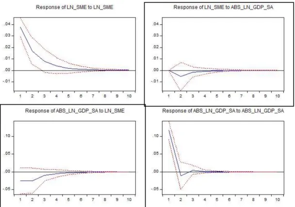
3.1.3.4.1 Impulse-Response Analysis (IR)
After obtaining the appropriate lag lengths in the VAR system, it is proceed to the next step that is called the IR function. IR functions demonstrate the effects of shocks on variables by using tables or graphics. Shocks have come into play and how the variables are willing to response these shocks are comprehended with the help of this process. In order to determine to shocks, the movements of the variables for 10 periods are examined first. With the help of graphics, the responses given by the other series with the change of 1 unit are determined. The same responses may be seen as a table. Columns express the variables that shocks come into play, while lines show the response of variables to these shocks (Tarı R. , Ekonometri , 2010).
34
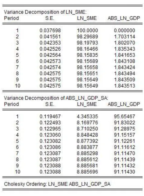
3.1.3.4.2 Variance Decomposition Analysis (VDC)
The variance decomposition finds out what percentage of changes in variable stems from its own and what percentage stems from other variables. It is described as an exogenous variable if it explains nearly one hundred percent of the variation in variance on its own. Sorting of variables in VDC is very crucial. Variables are sorted from external to internal. Variance decomposition is the second function that is aimed at VAR.
VDC examines what percentage of the variation that occurs in the variances of the variables are revealed by their own lags and what percentage is revealed by the other variables lags. It is further used as an extra evulation whether the variables are internal or external (Tarı R. , Ekonometri, 2006).
Unconstrained VAR models are not appropriate for short-term predictions when they are over-parametric. It is also very crucial that mutual relations between variables are revealed in understanding the characteristics of prediction errors. Prediction error variance decomposition refers to the dependence of the rate of motion on one runway to its own shocks against other shocks. If εxt shocks do not account for any prediction error variance of the Yt series in all horizon estimates, it means that the Yt series are external. If εxt explains all the variances of the prediction errors of the series Yt, Yt is called internal (Kutlar, 2000).
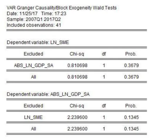
3.1.3.5 Granger Causality Test
While co-integration results indicate the existence of a long-term relationship between the variables, it makes no comment about the direction of relationship. On the other hand, variables in the VAR model must be sorted from external variables to internal variables. Economic relations are so complicated that internal and external discrimination of variables may not be possible. In that case, the Granger causality test is used to analyze the relationship between variables (Granger, 1969).
35
There may be a strong correlation between the two observed variables. However, it is not always possible for relationships to have causality. Although the regression analysis is interested in dependence on one variable to another, it does not have to be related to the causality of variables. No matter how strong or meaningful a statistical relationship is, it may not be perceived as a causal relationship.
Causality comes from a theory other than intellectual statistics (Gujarati, 1995).
Significant changes are made in the standard Granger causality test on the evolution of the time series analysis process. Accordingly, if the long-term cointegration is tested and the variables are cointegrated, then the lag value of the disturbance term of the long-term regression equation should be included in the Granger error correction model as an error correcting term. After that, Granger causality test should be performed.
If there is no cointegration relationship between variables, the Granger causality test should be continued without error correction. If there is a cointegration between variables, the standard applied Granger causality test is invalid and the error correction term definitely have to be added to the model.
Granger indicates that the causality relationship between two variables is modeled as follows:
Xt + b0 Yt = ∑𝑚𝑖=1 αi Xt –i + ∑𝑚𝑖=1 bi Yt –i + ε1
Yt + c0 Xt = ∑𝑚𝑖=1 ci Xt –i + ∑𝑚𝑖=1 𝑑i Yt –i + ε2
If b0 = c0 = 0 in the model, it is a basic causality model. In other words, the new model looks as follows:
Xt = ∑𝑚𝑖=1 αi Xt –i + ∑𝑚𝑖=1 bi Yt –i + ε1
36
The main idea of the concept of causality developed by Granger is that a cause does not come after a reason. Hence, if the variable x affects the variable y, the variable x also helps to improve the prediction of the variable y (Lütkepohl, 1993).
The Granger Causality Test assumes that if the information enables prediction of the variables in any VAR model, it exists within the time series of the variables. In general, as future does not predict past, if variable x is the Granger cause of variable y, changes in x are the pioneer of the changes in y. As a consequence, in a model prediction that y is a dependent variable, other variables and the historical values of y are independent variables, if historical values of x are also included in the model and these values affect statistically significant predictions of y, than x is the Granger cause of y. It is said that process is similar when if y is the Granger cause of x (Gujarati, 1995).
For above mentioned model the Granger causality test is performed as follows:
If the following H1 hypothesis cannot be rejected, x is not the cause of y.
H1 : b21= b22=…..b2p = 0
If the H2 hypothesis is rejected, y is not the cause of x.
H2 : d11= d12=…..d1p = 0
If both the H1 and H2 hypotheses are rejected, it can be inferred that there is a two-sided causality between x and y. In this case, it is said that there is a feedback effect.
The above hypothesis tests can be tested with the Wald test (F):
𝐹 = (𝐻𝐾𝑇𝑆 − 𝐻𝐾𝑇)/𝑟 𝐻𝐾𝑇/(𝑛 − 𝑘)
37
Where HKTS denotes the sum of error squares of the restricted model, HKT denotes the sum of error squares of the unrestricted model, r denotes the number of constraints, n denotes the number of observations and k denotes the number of modeled parameters. If the calculated F value is greater than the F table value, the H1 and H2 hypotheses are rejected.
The relationship between the two variables in the Granger Causality Test is four different types. In the case of causality between variables, this causality determines the direction of the relationship between variables. (Granger, 1969).
1- Causality
Assuming that σ 2 (X / U) <σ 2 (X / U -Y), if the sum of the squares of the error terms of the prediction which is obtained by using historical values of X and Y is smaller than the sum of the squares of the error terms of the prediction which is obtained by using historical values of X, There is an existence of causality from Y to X. (Y ⇒ X)
2- Feedback
If it is assumed that σ 2 (X / U) <σ 2 (X / U - Y) and σ 2 (Y / U) <σ 2 (Y / U - X), there is an existence of causality from Y to X and from X to Y. In other words, there is a two-sided causality. (Y⇔X)
3- Instantaneous Causality
Assuming σ 2 (X / U, Y) <σ 2 (X / U), it is said that there is always a causality from Y to X. If the current values of the Y's are added to the current value of the X's in the forecasting model, the sum of the error squares that is obtained from the estimation is reduced.
4- Causality Lag
In the case where σ 2 (X / U - Y (k)) <σ 2 (X / U - Y (k +1)) is assumed, the sum of the error squares obtained by adding the current values of Y to the model. It means that the current values of Y do not need to be added to the model since it would be larger than the sum of error squares.
38
CHAPTER 4
4 EMPIRICAL STUDY
4.1 Data Analysis
The three-month cash credits used for SMEs credits and quarter-annual data is used for GDP between January 2007 and June 2017. They are adjusted of inflation with the TÜFE 2003-based price index. After adjusting their ln returns are calculated.