Output Regulation for All-Pole and Minimum Phase LTI /
LTV Systems
a thesis
submitted to the department of electrical and
electronics engineering
and the institute of engineering and sciences
of bilkent university
in partial fulfillment of the requirements
for the degree of
master of science
By
Naci Saldı
June 2010
I certify that I have read this thesis and that in my opinion it is fully adequate, in scope and in quality, as a thesis for the degree of Master of Science.
Prof. Dr. ¨Omer Morg¨ul(Supervisor)
I certify that I have read this thesis and that in my opinion it is fully adequate, in scope and in quality, as a thesis for the degree of Master of Science.
Prof. Dr. A. B¨ulent ¨Ozg¨uler
I certify that I have read this thesis and that in my opinion it is fully adequate, in scope and in quality, as a thesis for the degree of Master of Science.
Assist. Prof. Ulu¸c Saranlı
Approved for the Institute of Engineering and Sciences:
Prof. Dr. Levent Onural
ABSTRACT
Output Regulation for All-Pole and Minimum Phase LTI /
LTV Systems
Naci Saldı
M.S. in Electrical and Electronics Engineering
Supervisor: Prof. Dr. ¨
Omer Morg¨
ul
June 2010
In this thesis, the problem of enabling the output of a system to track the refer-ence signals and reject the disturbances created by the same exogenous system is considered. This problem is widely known as Output Regulation Problem. Firstly, we propose a method for all-pole LTI systems by using relative degree property and then we apply the same method for minimum phase LTI systems along with some modifications. In order to obtain controllers for a minimum phase LTI case, the system is converted into an all-pole system by employing the inverse system as the first part of the controller. Then using the method that we used in all-pole cases, we obtain the second part of the controller. Combining these two controllers gives us an overall controller which solves the output regulation problem. This method for LTI systems is then extended to all-pole and
mini-mum phase LTV systems. However, in order to apply the same methodology we
have to make some assumptions on LTV systems. For minimum phase cases, the normal form is obtained by applying certain Lyapunov transformations and then minimum phaseness is defined in accordance with the normal form. Furthermore we show that, similar to minimum phase LTI cases, pole / zero cancelations oc-cur between the inverse system and the original system in minimum phase LTV
cases. The method that we develop depends on analytical calculation of the controller and gives a certain degree of freedom to change the transient behavior of the system by only changing some controller parameters.
Keywords: Output Regulation, Tracking, Disturbance Rejection, All-Pole,
Mini-mum Phase, Relative Degree, LTI System, LTV System, Pole / Zero Cancelation, Inverse System, Lyapunov Transformation
¨
OZET
T ¨
UM-KUTUPLU VE ENK ¨
UC
¸ ¨
UK EVREL˙I DO ˘
GRUSAL
ZAMANDA BA ˘
GIMSIZ VE DO ˘
GRUSAL ZAMANLA DE ˘
G˙IS
¸EN
S˙ISTEMLER˙IN C
¸ IKIS
¸ REG ¨
ULASYONU
Naci Saldı
Elektrik ve Elektronik M¨
uhendisli˘
gi B¨
ol¨
um¨
u Y¨
uksek Lisans
Tez Y¨
oneticisi: Prof. Dr. ¨
Omer Morg¨
ul
Temmuz 2010
Bu tezde T¨um Kutuplu ve Enk¨u¸c¨uk Evreli Do˘grusal Zamanda De˘gi¸smez Sistemlerin dı¸ssal bir sistem tarafından ¨uretilen referans sinyalini takibi ve aynı dı¸ssal sistem tarafından ¨uretilen bozucuların engellenmesi konusunu ince-lenmi¸stir. Bu problem literat¨urde C¸ ıkı¸s Reg¨ulasyonu olarak adlandırılır. ˙Ilk
olarak, T¨um Kutuplu(All-Pole) Sistemlerin g¨oreli derece ¨ozelli˘gini kullanarak
C¸ ıkı¸s Reg¨ulasyonu problemini ¸c¨ozmek i¸cin bir y¨ontem geli¸stirilmi¸stir ve aynı y¨ontem bazı de˘gi¸siklikler yapılarak Enk¨u¸c¨uk Evreli Do˘grusal Zamanda Ba˘gımsız sistemlere uygulanmı¸stır. Bu ¸c¨oz¨um¨u, Enk¨u¸c¨uk Evreli(Minimum Phase) sistem-lere uygulamak i¸cin, sistemin tersi, denetleyicinin ilk par¸cası olarak kullanılmı¸stır ve sistem T¨um Kutuplu hale getirilmi¸stir. Sonra, bu y¨ontemle denetleyicinin ikinci kısmı olu¸sturulmu¸stur. Bu par¸caları birle¸stirerek, reg¨ulasyon ko¸sullarını sa˘glayan toplam denetleyici elde edilmi¸stir. Bu y¨ontem daha sonra T¨um Ku-tuplu ve Enk¨u¸c¨uk Evreli Do˘grusal Zamanla De˘gi¸sen sistemlere geni¸sletilmi¸stir. Ancak, aynı y¨ontemi Do˘grusal Zamanla De˘gi¸sen sistemlere uygulamak i¸cin bazı varsayımlarda bulunmak gerekmektedir. Enk¨u¸c¨uk Evreli durum i¸cin belirli Lya-punov d¨on¨u¸s¨umleri uygulanarak sistem bir normal forma getirilmi¸stir ve bu
normal form ¨uzerinden Enk¨u¸c¨uk Evreli olmak tanımlanmı¸stır. Bunun yanısıra, Enk¨u¸c¨uk Evreli Do˘grusal Zamanda De˘gi¸smez sistemlere benzer olarak Enk¨u¸c¨uk Evreli Do˘grusal Zamanla De˘gi¸sen durumda ters sistem ve orjinal sistem arasında kutup / sıfır sadele¸smesinin oldu˘gu g¨osterilmi¸stir. Geli¸stirilen bu y¨ontem denet-leyicinin analitik olarak hesaplanmasına dayanmaktadır ve bu y¨ontem bazı denet-leyici de˘gi¸skenlerini de˘gi¸stirerek sistemin ge¸cici davranı¸sını de˘gi¸stirilebilmesine de olanak vermektedir.
Anahtar Kelimeler: C¸ ıkı¸s Reg¨ulasyonu, Takip, Bozulmaların Engellenmesi T¨um Kutuplu, Enk¨u¸c¨uk Evreli, G¨oreli Derece, Do˘grusal Zamanda Ba˘gımsız Sistemler, Do˘grusal Zamanla De˘gi¸sen Sistemler, Kutup / Sıfır Sadele¸smesi, Ters Sistem, Lyapunov D¨on¨u¸s¨um¨u
ACKNOWLEDGMENTS
Firstly, I would like to thank my supervisor Prof. Dr. Omer Morg¨¨ ul for his supervision, support and enlightening guidance throughout the development of this thesis.
I am grateful to thank Prof. Dr. A. B¨ulent ¨Ozg¨uler and Assist. Prof. Ulu¸c Saranlı for reading and commenting on this thesis.
I would also to thank my parents Muzaffer Saldı and S¸ahinde Saldı and my brother Necdet Saldı.
Finally, I would like to give special thanks to my fiance Rana Keskin whose endless support, encouragement and understanding made this study possible.
Contents
1 INTRODUCTION 1
2 OUTPUT REGULATION for ALL-POLE and MINIMUM
PHASE LTI SYSTEMS 9
2.1 Relative Degree Property . . . 11
2.2 Controller for All-Pole LTI Systems . . . 11
2.3 Observer Based Controller for All-Pole LTI Systems . . . 21
2.4 Controller for Minimum Phase LTI Systems . . . 23
2.5 Observer Based Controller for Minimum Phase LTI Systems . . . 34
2.6 Numerical Results . . . 37
2.6.1 Example 1 . . . 37
2.6.2 Example 2 . . . 41
2.6.3 Example 3 . . . 44
3 OUTPUT REGULATION for ALL-POLE and MINIMUM
PHASE LTV SYSTEMS 51
3.1 Relative Degree Property . . . 53
3.2 Controller for All-Pole LTV Systems . . . 54
3.3 Controller for Minimum Phase LTV Systems . . . 63
3.4 Pole/Zero Cancelation in LTV Systems . . . 99
3.5 Numerical Results . . . 105 3.5.1 Example 1 . . . 106 3.5.2 Example 2 . . . 108 3.5.3 Example 3 . . . 111 3.5.4 Example 4 . . . 114 3.5.5 Appendix . . . 116 4 CONCLUSION 119
List of Figures
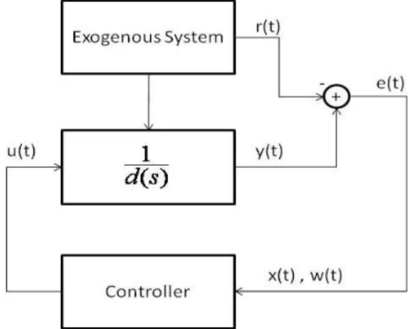
2.1 Overall System Block Diagram . . . 11
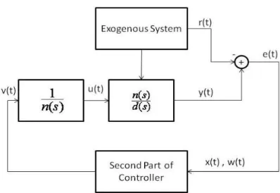
2.2 Overall System Block Diagram . . . 24
2.3 Tracking of Reference Signal . . . 39
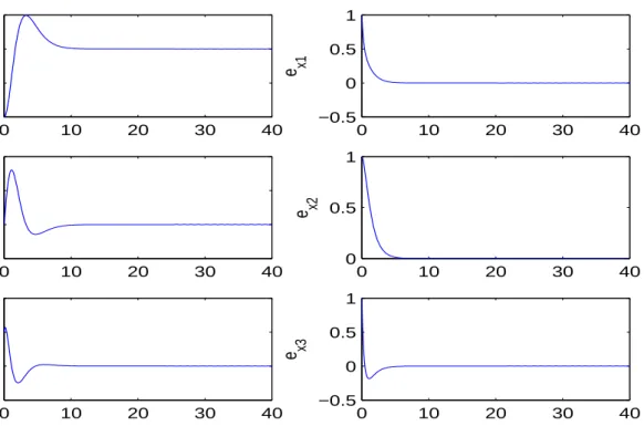
2.4 Stability of Closed-Loop System . . . 39
2.5 Error between x, w and ˆx, ˆw . . . 40
2.6 Tracking of Reference Signal . . . 42
2.7 Stability of Closed-Loop System . . . 43
2.8 Error between x, w and ˆx, ˆw . . . 43
2.9 Tracking of Reference Signal . . . 46
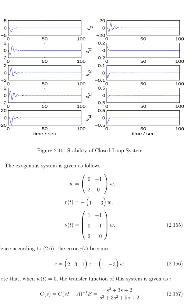
2.10 Stability of Closed-Loop System . . . 47
2.11 Error between x, w and ˆx, ˆw . . . 48
2.12 Tracking of Reference Signal . . . 49
2.13 Stability of Closed-Loop System . . . 50
3.1 Tracking of Reference Signal . . . 107
3.2 Stability of Closed-Loop System . . . 108
3.3 Tracking of Reference Signal . . . 110
3.4 Stability of Closed-Loop System . . . 111
3.5 Tracking of Reference Signal . . . 113
3.6 Stability of Closed-Loop System . . . 114
3.7 Tracking of Reference Signal . . . 116
Chapter 1
INTRODUCTION
In control theory, designing controllers that force the system to track a given reference signal r(t) and reduce (if possible, reject) the effect of unwanted signal
ν(t) (disturbance) at the output is among the most important problems [1–18].
This problem, which is generally referred to as the output regulation problem, was studied by many researchers and is still under investigation by considering all possible aspects of the problem. For this problem, some of the researchers take into account either disturbance rejection or reference signal tracking only [3–6]. Alternatively, some of the researchers worked on both the disturbance rejection and the reference signal tracking problem simultaneously [7], [8]. Furthermore, in this formulation some of the researchers assumed that the reference signals and the disturbances are considered the signals which are generated by different dynamical systems. In the latter case, these dynamical systems are assumed to be separate as shown below :
˙ν(t) = S1ν(t),
˙r(t) = S2r(t). (1.1)
where r(t) and ν(t) are the reference and disturbance signals, respectively, and
the formulation of the output regulation problem, we will try to find a controller structure to track the reference signal and to reject the disturbances simultane-ously. Instead of the model given by (1.1), we will assume that the reference signal r(t) and the disturbance signal ν(t) are generated by the same dynamical system, which is called as the exogenous system [9–11, 19–23]. The dynamics of the exogenous system is assumed to be as given below :
˙
w(t) = Sw(t), r(t) = Qw(t),
ν(t) = P w(t). (1.2)
where w(t) is called the exogenous signal, S, Q and P are matrices which have appropriate dimensions. Note that, even if the reference signal and disturbances have distinct dynamic behaviors as given in (1.1), one can still transform (1.1) into the form given by (1.2) as shown below :
w˙1 ˙ w2 = S1 0 0 S2 w1 w2 , r(t) = ( I 0 ) w1 w2 , ν(t) = ( 0 I ) w1 w2 . (1.3)
As can be seen, (1.3) has the same form as given by (1.2) where S = S1 0 0 S2 , Q = ( I 0 ) , P = ( 0 I )
[24]. One disadvantage of using (1.3) instead of (1.1) might be the following: the pairs (Q, S) and (P, S) in (1.3) are not observable. In the remaining of the thesis, we assume that the reference signal and disturbances are generated by the same dynamical system as given by (1.2). Note that the
state space form of plant for which we will design controllers is given below :
˙x(t) = A(t)x + B(t)u + ν, (1.4)
y(t) = C(t)x. (1.5)
where xϵℜn, uϵℜ, yϵℜ, νϵℜn represent the system state, input, output and dis-turbances .respectively and A(t)ϵℜn×n, B(t)ϵℜn×1, C(t)ϵℜ1×n represent system
matrices. If any of the system matrices is time-varying, then our system become linear time-varying. Conversely, if all of the system matrices are time-invariant, then our system becomes linear time-invariant.
In the output regulation problem, the objective is to find such a control law that the closed-loop system tracks the reference signal and rejects the distur-bances simultaneously. Actually, if the error is to be defined as the difference between the reference signal r(t) and the system output y(t), then output regu-lation problem can be converted into obtaining such a controller that the overall system satisfies the conditions given below [24]:
(i) For all the initial conditions of the original system and the exogenous sys-tem,
lim
t−→∞e(t) = limt−→∞(y(t)− r(t)) = 0. (1.6)
(ii) The closed-loop system is exponentially stable with w = 0.
Throughout the thesis, we will refer to the conditions (i) and (ii) given above as regulation conditions. Note that if the output regulation problem is de-fined as the tracking of the reference signal and the rejecting of the disturbances simultaneously, then any controller which solves the output regulation problem also satisfies the regulation conditions given above. Conversely, any controller which satisfies the regulation conditions given above also solves the output reg-ulation problem. This could be easily seen if the exogenous system given by (1.2) is combined with the closed-loop system dynamics. In this case, the state
transition matrix will have a block triangular form. By using this structure, the equivalence stated above can be shown easily [24].
The LTI part of this problem was studied by many authors. The first attempt to solve the problem of linear output regulation was made in [1] and [2] where the case of the constant reference signal and the disturbances was considered. In [9], a set of equations, called the regulator equations, were introduced and the controller which solved the output regulation problem was related to the solution of the regulator equations. In [10], a new concept the internal model principle was introduced which roughly stated that the controller which solved the output regulation problem included a model of exogenous system. In [11], polynomial matrices were used in the output regulation problem, and a primary condition, which was a single polynomial matrix formulation and that the controller should satisfy was given. In addition, the internal model principle ,which was first in-troduced in [10], was clarified by using polynomial matrices. The robust case of the linear output regulation problem was considered in [12–16]. In [12], the controller which solved the output regulation problem was shown to be robust to the perturbations in plant parameters and unmeasurable disturbances if and only if it regulated a system called the expanded system. Furthermore, in [15] the case which the disturbances were unmeasurable, arbitrary signals were con-sidered and two conditions for the solvability of the output regulation problem were given. The application of the frequency domain techniques for the output regulation problem can be found in [17, 18].
LTV case of the output regulation problem did not receive as much attention as its LTI counterpart did, possibly due to the mathematical difficulties which may be encountered in the analysis. In [19], the linear periodic time-varying exogenous system and the LTI plant case were studied. Differential regulator matrix equations which were the counterparts of the regulator equations in LTI cases were found. In [20], the case of minimum phase time-varying systems with
a time-varying exogenous system were considered and a differential type of reg-ulator equations were found for the solvability of the output regulation problem. Then, in [21] a general time-varying system with a time-varying exogenous sys-tem was considered and differential regulator equations were derived as in the previous cases.
For the solution of the output regulation problem for nonlinear systems, the researchers mainly tried to extend the existing approaches for linear systems to nonlinear cases. In [25], the internal model principle was extended to the non-linear systems defined on differentiable manifolds. In [26], a PI controller was employed for the constant disturbances and the reference signal case. In [27], the work in [9] for linear multivariable systems was extended to the nonlinear setting with slowly varying or constant exosystem and nonlinear equations ,which were the nonlinear counterparts of the linear regulator equations in a special case, were obtained. Then, in [22] the results of [9] was extended to a general setting in which the exosystem was a time-varying nonlinear system. In the latter, the nonlinear regulator equations were obtained and their solution guaranteed the solution of the output regulation problem. After the work in [22], solvability con-ditions for these nonlinear regulator equations were studied by many researchers, see e.g. [22,23,28,29]. In [30,31] the case of nonlinear system with nonhyperbolic zero dynamics was studied. In [32], the results in [22] were extended to the feed-back linearizable system. In [33], the global robust output regulation with error feedback was considered. In [34], internal models were used to design output regulators for nonlinear systems. In [35], global output regulation of uncertain nonlinear systems was studied and a novel high gain internal model was devel-oped.
In most of the existing approaches for the output regulation problem, one tries to obtain a control law which satisfies (i) assuming that (ii) is satisfied. Thus, in the classical approach, one assumes that the closed-loop system is al-ready exponentially stable and consequently one tries to find a controller which
satisfies the regulation condition (i). Additionally, the existing solutions for the reduced problem do not give the controller explicitly. Instead, in the classical approach one obtains a set of equations, called the regulator equations [24], and the solvability of the output regulation problem depends on the solvability of the regulator equations. The regulator equations for LTI cases are shown below :
XcS = AcXc+ Pc,
0 = CcXc+ Qc (1.7)
where Ac, Pc, Cc and Qc are the closed-loop system state transition matrix,
disturbance matrix, output matrix and reference signal matrix, respectively [24]. Here, Xc is the unknown matrix to be found, and once Xc is found, one can design
a controller by using Xc. Note that (1.7) is called as the Sylvester equations. For
details, see [24]. If one uses the same approach in LTV cases, the regulator equations become as follows :
˙
Xc(t) + Xc(t)S(t) = Ac(t)Xc(t) + Pc(t),
0 = Cc(t)Xc(t) + Qc(t) (1.8)
where Ac, Pc, Cc and Qc are the closed-loop system state transition matrix,
dis-turbance matrix, output matrix and reference signal matrix, respectively [20]. As in LTI cases, here Xc(t) is the unknown matrix, and if one finds a solution, then
by using Xc(t) one can construct a controller. Note that (1.8) is also called the
differential Sylvester equations. For more details, refer to [20]. The fulfillment of
these equations corresponds to the fulfillment of the condition (i).
In this thesis, we restrict ourselves only to all-pole and minimum phase sys-tems. Since we deal with only some portion of the general systems, our proposed method has advantages over the existing approaches. The advantages of our solution to the output regulation problem are as follows;
• Different from existing approaches our solution depends on the analytical
This analytical calculation particularly is very important for LTV systems because finding controller by using regulator equations, which include a differential matrix equation, is a very difficult task.
• Our approach does not assume the fulfillment of the condition (ii) like
most of the existing approaches do. Instead, we propose a controller which satisfies the conditions (i) and (ii). Moreover, in our approach rather than a single controller, a class of controllers which solve the output regulation problem is constructed.
• In LTI case, the controller that solves the output regulation problem may
be found easily by using regulator equations. However, in this methodology we do not have enough degree of freedom to alter the transient behavior of the system. On the other hand, our approach allows one to alter the transient behavior of the closed-loop system upto a certain degree only by changing some controller parameters. By this way, the designer can achieve some desired specifications other than the regulation conditions.
The outline of this thesis is as follows;
In chapter 2, we study the output regulation problem for all-pole and min-imum phase LTI systems. First of all, the problem formulation will be given. Then, by defining and using the relative degree property of the LTI systems, a static controller for all-pole systems will be obtained. In addition, observers for the original system and the exogenous system will be designed and combined with the overall system. Afterwards, we consider the minimum phase systems and define minimum phaseness. By introducing an inverse system, a dynamic controller for minimum phase case will be achieved. Then, similar with all-pole cases, observers will be designed for both the original system and the exogenous system. Finally, we will show some numerical results.
In chapter 3, we will extend the technique in chapter 2 to the output regu-lation problem for the all-pole and the minimum phase LTV systems. First the
problem formulation will be given. Then, by defining and employing relative de-gree property, controller for all-pole systems will be constructed. After that, the inverse systems of the minimum phase LTV systems will be found by applying certain transformations on the original systems. Then, a dynamic controller for the minimum phase systems will be obtained by using the inverse systems as a first part of the controller. Then we will show pole/zero cancelations between the inverse system and the original system. Lastly, some numerical results are shown.
In the section which we will deal with controller design for minimum phase LTV systems, we will use pole/zero definitions of LTV systems and we will try to show pole/zero cancelations between the inverse systems and the original sys-tems. However, in literature there are no unique definition of poles and zeros for LTV systems. Thus, to show pole/zero cancelations we will use definitions of poles and zeros in [36] and these definitions are the generalizations of pole/zero definitions for LTV systems in [37]. In [37], definition of poles and zeros for special class of time-varying systems were given. In these definitions, zeros cor-responds to the modes that make output zero when we apply this as an input to the system and poles correspond to the modes which determine the stability of the system. However, in [36] definition of poles and zeros for a general class of time-varying systems were given. Additionally, there are two different zero definition in [36] which are transmission zeros and ordinary zeros. The
transmis-sion zeros correspond to the transmistransmis-sion zeros of the MIMO systems and the ordinary zeros correspond to the zeros of the SISO systems in LTI cases.
In the last chapter, we conclude our remarks by going over some important points of the output regulation problem, and we propose some further research areas, as well as some possible extensions of our results.
Chapter 2
OUTPUT REGULATION for
ALL-POLE and MINIMUM
PHASE LTI SYSTEMS
Throughout this section, we consider single-input-single-output (SISO) linear-time-invariant (LTI) systems which have the following form :
˙
x(t) = Ax + Bu + ν, (2.1)
y(t) = Cx, (2.2)
where xϵℜn, yϵℜ, uϵℜ represent the system state, output and input respectively and Aϵℜn×n, Bϵℜn×1, Cϵℜ1×n represent constant system matrices. We assume
the exogenous system that we deal with is in the form which is given below :
˙
w(t) = Sw(t), (2.3)
r(t) =−Qw(t), (2.4)
ν(t) = P w(t), (2.5)
where wϵℜm, dϵℜn and rϵℜ represent exogenous system states, disturbance sig-nals and reference signal respectively and Sϵℜm×m, P ϵℜn×m, Qϵℜ1×m represent
constant matrices of exogenous system. The sign ”-” in the equation that gives reference signal (2.4) is chosen to ensure compliance with the use in the literature. Then, the tracking error e(t) can be defined as shown below :
e(t) = y(t)− r(t) = Cx + Qw. (2.6)
In order to use the system states x(t) and the exogenous system states w(t) in the controller, we should make the assumption of the observability for both of the systems.
Assumption 1. The pairs (C, A) and (Q, S) are both observable. Assumption 2. S has distinct eigenvalues with zero real parts
Assumption 2 guarantees that the solutions of the exogenous system are bounded and do not decay to zero as time goes infinity. If the exogenous system has eigenvalues with negative real parts, then the reference signal or/and the disturbances may decay to zero. But, decaying reference signal or disturbances are not considered in the output regulation problem which is investigated here. Conversely, if the exogenous system has eigenvalues with positive real parts, then the reference signal and the disturbances become unbounded, but it is not con-sidered here for simplicity.
Our objective is to design a feedback control law by using both the original and the exogenous system states such that the closed-loop system satisfies the regulation conditions (i) and (ii). In the simplest form (All-Pole case), we will use the relative degree property of the system in order to find the controller which provides regulation conditions. Therefore we need to define this property first.
2.1
Relative Degree Property
If the system satisfies the following conditions :
CA = CAB = . . . = CAr−2B = 0, (2.7)
CAr−1B = α̸= 0 , r ≤ n, (2.8)
then the system has a ”relative degree r”. If we take the derivative of the output of the system y(t), input u(t) appears at the rthderivative because of the relative
degree property : i.e.
˙
y = C(Ax + Bu) = CAx + CB|{z} u,
.. .
y(r−1) = CAr−2(Ax + Bu) = CAr−1x + CA| {z } u,r−2B
y(r) = CAr−1(Ax + Bu) = CArx + CAr−1Bu = CArx + αu. (2.9) The parts, indicated by underbrace are equal to zero. Therefore, this property of the system can be used to design controllers for All-Pole systems.
2.2
Controller for All-Pole LTI Systems
If we have a system that is full-relative degree (i.e. r = n and system di-mension is n), then this system is called as an ”All-Pole System”. Transfer function of this kind of systems are expressed as follows : G(s) = d(s)1 where
d(s) = sn+ α
n−1sn−1+ . . . + α1s + α0. A state space model of the system of this
type can be given as shown below:
˙x = 0 1 0 0 . . . 0 0 0 1 0 . . . 0 .. . . .. ... ... ... −α0 −α1 . . . −αn−2 −αn−1 x + 0 0 .. . 1 u, y = ( 1 0 . . . 0 ) x. (2.10)
Remark 1. Using the system model given by (2.10), the proof of full-relative
degree property of the system can be done easily.
If we take the derivative of the error given by (2.6) repeatedly, and if we use the system equations given by (2.1)-(2.5) and the equations given by (2.7)-(2.8) with r = n, then we obtain the following equations :
e = Cx + Qw, ˙e = C ˙x + Q ˙w, = C(Ax + Bu + P w) + QSw, = CAx + (CP + QS)w, ¨ e = CA ˙x + (CP + QS) ˙w, = CA2x + CAP w + (CP + QS)Sw, .. . e(n)= CAnx + αu + CAn−1P w + Sn−1Sw, (2.11)
where in the derivatives we used the relative degree property given by (2.7)-(2.8). Here we have α = CAn−1B ̸= 0 (see (2.8)), and the matrices Si are given as below
:
Si = Si−1S + CAi−1P, S0 = Q, 1≤ i ≤ n , (2.12)
In this case, we can choose the following control law for u(t) :
u = 1
α{−CA
nx− S
nw− Ln−1en−1− . . . − L1˙e− L0e}. (2.13)
By using (2.6) in (2.11) and by separating the multipliers of x and w, we can rewrite (2.13) as follows :
u = Kxx + Kww, (2.14)
where Kx and Kw are given as below :
Kx =− 1 α(CA n+ L n−1CAn−1+ . . . + L1CA + L0C), (2.15) Kw =− 1 α(Sn+ Ln−1Sn−1+ . . . + L1S1+ L0Q). (2.16)
Thus, when equation (2.13) is substituted into equation (2.11), we get the fol-lowing error dynamics :
e(n)+ Ln−1e(n−1)+ . . . + L1˙e + L0e = 0 (2.17)
If we use Laplace transformation, the characteristic polynomial of equation (2.17) will be as follows :
ch(s) = sn+ Ln−1sn−1+ . . . + L1s + L0. (2.18)
Hence, the polynomial given by (2.18) can always be made stable by choosing ap-propriate controller coefficients Li. In this case, the solution of the error dynamics
given by (2.17) is exponentially stable. Thus, if Li parameters are selected to
make the characteristic equation (2.18) exponentially stable in controller given by equation (2.13), then the regulation condition (i) is satisfied. In order to show regulator problem has been resolved with the controller given by (2.13), the second regulator condition (ii) should be satisfied as well. If the system in the equations (2.1)-(2.2) and the controller in the equations (2.13)-(2.14) are put
together, we will obtain the closed-loop system state space form as shown below :
˙x = (A + BKx)x + (P + BKw)w = Aclx + (P + BKw)w, (2.19)
e = y− r = Cx + Qw. (2.20)
Lemma 1. The static controller
u = Kxx, (2.21)
where Kx =−α1(CAn+ Ln−1CAn−1+ . . . + L1CA + L0C) makes the closed-loop
system (2.19)-(2.20) with w = 0 exponentially stable and characteristic equation of Acl matrix in (2.19) is given by (2.18).
In order to prove Lemma 1, we use the following fact.
Fact 2. For A, B, C given by system (2.10), the following holds :
BCAi = ( 0 . . . 0 ei+1 )T , (2.22) where 0≤ i ≤ n−1, 0 = 0 .. . 0
ϵℜn and ei+1ϵℜn is unit vector with (i + 1)th entry
is one.
Proof. In order to show this fact, we use mathematical induction.
When i = 0 BC = 0 .. . 0 1 ( 1 0 . . . 0 ) = ( 0 . . . 0 e1 )T . (2.23)
When i=m, BCAm =( 0 . . . 0 em+1 )T is true. Then, BCAm+1 = ( 0 . . . 0 em+1 )T 0 1 0 0 . . . 0 0 0 1 0 . . . 0 .. . . .. ... ... ... −α0 −α1 . . . −αn−2 −αn−1 , = ( 0 . . . 0 em+2 )T . (2.24)
Thus, the above statement is true by mathematical induction.
Then, the proof of Lemma 1 is given by using the above fact shown below.
Proof. If we combine the controller (2.14) with the system (2.1), the closed-loop
system is obtained with w = 0. Then, the closed-loop system is given by :
˙x = Ax + BKxx = (A + BKx)x = Aclx, (2.25)
where
Acl = A− BCAn− Ln−1BCAn−1− . . . − L1BCA− L0BC. (2.26)
By using Fact 1, we can find Acl as follows :
First we construct BCAn with the help of the Fact 1 :
BCAn= ( 0 . . . 0 en )T 0 1 0 0 . . . 0 0 0 1 0 . . . 0 .. . . .. ... ... ... −α0 −α1 . . . −αn−2 −αn−1 , = ( 0 . . . 0 a )T . (2.27) where a = ( −α0 . . . −αn−1 )T
. Now we know BCAi for 0 ≤ i ≤ n − 1 from the Fact 1. Hence if we substitute this result and (2.27) into (2.26), the following
form is obtained for Acl : Acl = 0 1 0 0 . . . 0 0 0 1 0 . . . 0 .. . . .. ... ... ... −L0 −L1 . . . −Ln−2 −Ln−1 . (2.28)
If we constitute the characteristic equation of Acl, it turns out that it is the
same as (2.18) . In addition, in order to make error e(t) exponentially stable Li
coefficients were chosen such that (2.18) became a Hurwitz polynomial. Hence, this shows that Acl matrix is a Hurwitz matrix and the closed-loop system with
w = 0 is exponentially stable.
If the results of the equation (2.17) and Lemma 1 is used, the following theorem can be obtained.
Theorem 3. The static controller given by equations (2.13)-(2.14) satisfies the
regulation conditions (i.e. (i) and (ii)) for the system in the form (2.1)-(2.5) with the system matrices (2.10).
Proof. (i) From the equations (2.17) and (2.18), it turns out that the error e(t) is exponentially stable (i.e. |e(t)| < k exp−λt). Hence,
lim
t→∞|e(t)| = 0. (2.29)
(ii) With w = 0 Lemma 1 showed that the closed-loop system is exponentially stable. i.e.
Re{eig(Acl)} < 0
where eig(Acl) denotes the eigenvalues of Acl in (2.26) and (2.28).
These two results point out that regulation conditions are satisfied with static controller given by equations (2.13).
Remark 2. As we mentioned in Chapter 1, linear output regulation problem
has been studied extensively in the past. Most of the existing approaches rely on obtaining set of regulator equations which should be satisfied by the controllers in order to solve the regulator problem. In these approaches, the second part of the regulator conditions (ii) is assumed to be true and the problem is reduced to finding the controller part associated with the exogenous system states, if the controller is a static one. In all-pole case that we deal with above, this corresponds to finding Kw assuming that Kx is known. In this case, regulator equations
become as given below :
XcS = (A + BKx)Xc+ (P + BKw), (2.30)
0 = CXc+ Q. (2.31)
If there exists a unique matrix Xc and Kw that satisfies above regulator equations,
then the first part of the regulator conditions (i) is satisfied by the controller which is given by below form :
u = Kxx + Kww (2.32)
In our approach, the static controller u = Kxx makes the closed-loop system
exponentially stable when the exogenous signal is not present, i.e. when w(t) =
0. Actually, we can assign poles of the closed-loop system with this controller
anything that we desire because the coefficients of the characteristic polynomial of the closed-loop system given by (2.18) depend only on the controller parameters Li. Thus, this shows that the static controller class given by the equation (2.13)
covers all the static controllers that can be designed to make the closed-loop system (2.19)-(2.20) stable without the exogenous system. In addition to this, Kw part
of the controller in equation (2.13) can be achieved from the regulator equations (2.30)-(2.31) as will be shown below.
Lemma 4. If we take the controller part Kx associated with the system states x(t)
w(t) in (2.13)-(2.14) which is given by (2.16) can be obtained from regulator equations (2.30)-(2.31).
Proof. We know that Kx is in the following form : Kx =−α1(CAn+Ln−1CAn−1+
. . . + L1CA + L0C). Let us try to find Kw from the equations (2.30)-(2.31) by
using the relative-degree property. For simplicity, we take α in (2.8) as 1. The first thing that we observe from (2.30)-(2.31) is the following :
e(i)= CAix− CAiXcw, (2.33)
where 0≤ i ≤ n − 1. We can prove (2.33) by mathematical induction. We first show that (2.33) is true for i = 0. From (2.20) we have
e = Cx + Qw. (2.34)
On the other hand, from (2.31) we obtain Q = −CXc. By using this in (2.34)
we obtain the following :
e = Cx− CXcw, (2.35)
which shows that (2.33) holds for i = 0. Now, assume that (2.33) holds for i = m, i.e. assume that the following holds :
e(m) = CAmx− CAmXcw. (2.36)
Then by differentiating (2.36) once more, we obtain :
e(m+1) = CAm˙x− CAmXcw = CA˙ m+1x + CAmBu + CAmP w− CAmXcSw,
= CAm+1x + CAmP w− CAmXcSw, (2.37)
from the relative degree property. If we multiply (2.30) with CAm, then the
following equation is obtained :
CAmXcS = CAm(A + BKx)Xc+ CAm(P + BKw) = CAm+1Xc + CAmP
where to obtain the last equality we used the relative degree property, see (2.7) and (2.8). Hence, we have the following :
CAmXcS = CAm+1Xc+ CAmP. (2.39)
If we substitute (2.39) into (2.37), then we obtain :
e(m+1) = CAm+1x + CAmP w− (CAm+1Xc+ CAmP )w,
= CAm+1x− CAm+1Xcw. (2.40)
Hence, by mathematical induction the statement (2.33) is true. Secondly, we observe that :
Si =−CAiXc, (2.41)
where Si are given by (2.12) and 0≤ i ≤ n. We can again prove this observation
by mathematical induction. We first show that (2.41) holds for r = 0. Indeed, from (2.12) we see that S0 = Q. On the other hand, from (2.31) we obtain :
S0 = Q =−CXc, (2.42)
which shows that (2.41) holds for i = 0. Assume that (2.41) holds for i = m, i.e. we have :
Sm =−CAmXc. (2.43)
Then, by using (2.43) in (2.12) we obtain :
Sm+1 =−CAmXcS + CAmP = (−CAm+1Xc− CAmP ) + CAmP,
=−CAm+1Xc, (2.44)
where we used (2.39) to obtain the final equality. Hence, by mathematical in-duction we show that (2.41) holds.
Let us use (2.33) for i = n− 1, i.e.
If we differentiate (2.45) with respect to time, and use (2.3) and (2.19), we obtain :
e(n) = CAn−1[(A− BKx)x + (P − BKw)w]− CAn−1XcSw. (2.46)
Assuming α = CAn−1B = 1 (without loss of generality), we obtain :
e(n)= CAnx− Kxx + CAn−1P w− Kww− CAn−1XcSw. (2.47)
By using (2.41) for i = n− 1 in (2.47), we obtain :
e(n)= CAnx− Kxx + CAn−1P w− Kww + Sn−1Sw. (2.48)
Finally, by using (2.12) for i = n in (2.48), we obtain :
e(n)= CAnx− Kxx− Kww + Snw. (2.49)
Hence, when Kx is given by (2.15), then Kw can be obtained from the regulator
equations (2.30)-(2.31) as given below :
−Kww = e(n)− CAnx + Kxx− Snw. (2.50)
Now let us consider the control law obtained by our approach, which is given by (2.13)-(2.14). If we use the latter in (2.11), we obtain :
e(n)= CAnx− Kxx− Kww + CAn−1P w + Sn−1Sw. (2.51)
By using (2.12) for i = n in (2.51), we obtain :
−Kww = e(n)− CAnx + Kxx− Snw. (2.52)
By comparing (2.52) and (2.50), we see that the term Kww obtained both by our
approach and by the regulator equations are the same. Hence, we conclude that if Kx is as given by (2.15), then Kw , which is obtained by our approach, is the
2.3
Observer Based Controller for All-Pole LTI
Systems
In order to implement the controller given by equations (2.13)-(2.14), in addition to error term e(t) and various derivatives of it, the signals w(t), x(t) should also be measurable. If only the system output y(t) and the reference signal r(t) are known, we can design observers for x(t) and w(t) through Assumption 1 and the outputs of these observers can be used in the controller equations (2.13)-(2.14). In the following, we will use the standard full order observer, also known as Luenberger observer [38], for our observer based controller design.
The observer structure for x(t) is in this below form :
ˆ
x = Aˆx + Bu + Lx(y− C ˆx + P ˆw), (2.53)
and the observer structure for w(t) is given by the below equations :
ˆ
w = S ˆw + Lw(r + Q ˆw), (2.54)
Let us define new state variables ex and ew as shown below :
ex = x− ˆx , ew = w− ˆw. (2.55)
Then, the dynamic equations of the above states can be found as follows :
˙ ex = ˙x− ˙ˆx = Ax + Bu + P w− Aˆx − Bu − P ˆw− LxCx + LxC ˆx ˙ ex = (A− LxC)ex+ P ew (2.56) and ˙ ew = ˙w− ˙ˆw = Sw− S ˆw + LwQw− LwQ ˆw = (S + LwQ)ew (2.57)
Since both (A, C) and (Q, S) pairs are observable, we can find Lx and Lw
ˆ
x, ˆw converge true states x, w exponentially. If we combine the system in the
equations (2.1)-(2.5) and the controller (2.13)-(2.14) with the observer equations (2.56)-(2.57), overall system can be obtained. The overall system (i.e. observer-controller-plant) state space model with states ex, ew become in the following
form : ˙x ˙ ex ˙ ew = (A + BKx) −BKx −BKw 0 (A− LxC) P 0 0 S + LwQ x ex ew + P + BKw 0 0 w, (2.58) e = ( C 0 0 ) x ex ew + Qw. (2.59)
Lemma 5. The system in equations (2.58)-(2.59) satisfies regulation conditions
(i) and (ii).
Proof. (i) Since the error e(t) is exponentially stable with controller (2.13), the controller-plant system (2.19)-(2.20) satisfies the regulator equations (2.30)-(2.31) and its inverse is also true. Thus, if the system in (2.58)-(2.59) satisfies regulator equation formed by its system matrices, then the error term e(t) is exponentially stable. The regulator equations formed by the matrices in (2.58)-(2.59) as follows :
Xc1 Xc2 Xc3 S = (A + BKx) −BKx −BKw 0 (A− LxC) P 0 0 S + LwQ Xc1 Xc2 Xc3 + P + BKw 0 0 , (2.60) 0 = ( C 0 0 ) Xc1 Xc2 Xc3 + Q. (2.61)
If Xc2 and Xc3 are chosen as zero vectors, then the regulator equations are
reduced to this below form :
Xc1S = (A + BKx)Xc1+ (P + BKw), (2.62)
0 = CXc1+ Q. (2.63)
The equations (2.62)-(2.63) are the same with regulator equations given by (2.30)-(2.31). Also in Lemma4, we proved that the regulator equations given by (2.30)-(2.31) are satisfied with the controller given by (2.13)-(2.14). This implies that the equations (2.62)-(2.63) have a solution. Thus, the regulator equations given by (2.60)-(2.61) are satisfied. This indicates that the error
e(t) exponentially decays to zero for the system given by the state space
representation (2.58)-(2.59).
(ii) The closed-loop state transition matrix with w = 0 is in block triangular form as can be seen in equation (2.58). In addition, the matrices (A+BKx),
(A− LxC) and (S + LwQ) are known to be Hurwitz. We know that the
state transition matrix eigenvalues are composed of these three matrices eigenvalues because of the block triangular structure as shown below: i.e
eig(Acl) = eig(A + BKx)
∪
eig(A− LxC)
∪
eig(S + LwQ), (2.64)
It easily follows that the closed-loop matrix in (2.58) is Hurwitz, which means that the closed-loop system with w = 0 is exponentially stable.
2.4
Controller for Minimum Phase LTI Systems
In general, the transfer function of LTI systems are as follows : G(s) = n(s)d(s). If the zeros of the system, i.e. the roots of n(s), are on the left-half-plane (LHP), this system is called as a ”Minimum Phase System”. Besides, these systems have
Figure 2.2: Overall System Block Diagram
relative degree r and r is given by r = (number of poles)− (number of zeros) . In order to obtain a state space model for such systems, suppose that n(s) and
d(s) are given as follows :
n(s) = sm+ bm−1sm−1+ . . . + b1s + b0, (2.65)
d(s) = sn+ αn−1sn−1+ . . . + α1s + α0. (2.66)
In this case, the system to be controlled can be given as shown below :
˙x = 0 1 0 0 . . . 0 0 0 1 0 . . . 0 .. . . .. ... ... ... −α0 −α1 . . . −αn−2 −αn−1 x + 0 0 .. . 1 u, y = ( b0 b1 . . . 1 0 . . . 0 ) x. (2.67)
We know that the zeros of the minimum phase system are stable. Then to make the system in (2.67) equivalent to an all-pole system, we can employ C1(s) = n(s)1
as the first part of the controller. Since there is no unstable pole/zero cancelations between C1(s) and the system in (2.67), the first part of the controller does not
cause any instability problem. The overall system will become equivalent to all-pole with this first part of the controller and a state space model for C1(s) can
be given as follows : ˙ ξ = 0 1 0 0 . . . 0 0 0 1 0 . . . 0 .. . . .. ... ... ... −b0 −b1 . . . −bm−2 −bm−1 ξ + 0 0 .. . 1 v = Gξ + Hv, (2.68) u = ( 1 0 . . . 0 ) ξ = Kξ, (2.69)
where ξϵℜm, vϵℜ and uϵℜ denote the controller states, input and output
re-spectively. Then Gϵℜm×m, Hϵℜm×1, Kϵℜ1×m, given by (2.68)-(2.69), represent constant system matrices . If we form the overall system by combining the orig-inal system in the equations (2.1)-(2.5) and the first part of the controller given by (2.68)-(2.69), a state space model of augmented system becomes in the form given below : ˙x ˙ ξ = A BK 0 G x ξ + 0 H v + P 0 w, (2.70) e = ( C 0 ) x ξ + Sw. (2.71)
This overall system has dimension ˜n = n + m where m is the dimension of the
inverse system C1(s). Since the poles of C1(s) and the zeros of the system in
(2.67) are canceled each other, the number of m unobservable states arise in the overall system given by (2.70)-(2.71).
Fact 6. The system given by (2.70)-(2.71) has relative degree n.
Proof. The first part of controller has transfer function C1(s) = n(s)1 and we know
from section (1.2) that this kind of transfer functions represent all-pole systems. Since the first part has dimension m, the system in (2.68)-(2.69) has relative degree m : i.e.
KH = KGH = . . . = KGm−2H = 0, (2.72)
In addition, the original system in (2.67) has relative degree r, thus the following equations must hold :
CB = CAB = . . . = CAr−2B = 0, (2.74) CAr−1B = γ ̸= 0. (2.75) Let us denote z = x ξ , Ac = A BK 0 G , Cc = ( C 0 ) and Bc = 0 H . Then, Cc = ( C 0 ) , CcAc = ( C 0 ) A BK 0 G = (CA CBK ) , CcA2c = ( CA CBK ) A BK 0 G =(CA2 CABK + CBKG ) , .. . CcArc = ( CAr CAr−1BK + CAr−2BKG + . . . + CBKGr−1 ) = ( CAr CAr−1BK ) , .. . CcAnc−2 = ( CAn−2 CAn−3BK + . . . + CAn−m−2BKGm−1+ . . . + CBKGn−3 ) = ( CAn−2 CAn−3BK + . . . + CAr−1BKGm−2 ) , CcAnc−1 = ( CAn−1 CAn−2BK + . . . + CAn−m−1BKGm−1+ . . . + CBKGn−2 ) = ( CAn−1 CAn−2BK + . . . + CAr−1BKGm−1 ) . (2.76)
where we used (2.74) and the fact that r = n−m. If we multiply these equations from right with Bc, we obtain the following result :
CcAcBc = 0, CcA2cBc = 0, .. . CcAnc−2Bc = 0, CcAn−1c Bc = βγ = ρ̸= 0,
where we used (2.72), (2.73) and (2.75). This proves that the overall system in (2.70)-(2.71) has relative degree n.
Thus, as in all-pole systems the input appears at the nth derivative of the
error e(t) which is shown below :
˙e = Cc˙˜x + Qw,
= CcAcx + C˜ | {z }cBcv + CcPc + QSw,
.. .
e(n) = CcAncx + βv + C˜ cAcn−1Pcw + ˜Sn−1w, (2.77)
where ˜Si = ˜Si−1S + CcAci−1Pc, 1 ≤ i ≤ n, ˜S0 = Q, and the part, indicated by
underbrace is equal to zero. In order to find the second part of the controller that guarantees the regulation conditions, we will use the same methodology, that we applied in all-pole systems. Therefore, we will choose control input u(t) as follows :
v = 1
γ{−CcA
n
cx˜− ˜Snw− ˜Ln−1en−1− . . . − ˜L1˙e− ˜L0e}. (2.78)
If the equation in (2.78) is substituted into equation in (2.77), we obtain the error dynamics e(t) as shown below :
The latter is the same with (2.17) that was obtained for all-pole systems. If we again use Laplace transformation, the characteristic polynomial of the equation (2.79) will be as given below :
ch(s) = sn+ ˜Ln−1sn−1+ . . . + ˜L1s + ˜L0 = 0. (2.80)
If the controller parameters{˜Ln−1, . . . , ˜L1, ˜L0} are chosen properly, we can make
the error e(t) exponentially stable as we discussed in Section 1.2. Actually, the second part of the controller is like a static controller and its state space model can be shown as follows :
v = Kξξ + Kxx + Kww. (2.81)
In this case, if we combine the first and the second part of the controller given by (2.68)-(2.69), (2.81) respectively, the overall controller becomes as shown below :
˙
ξ = (G + HKξ)ξ + HKxx + HKww,
u = Kξ. (2.82)
Thus, the closed-loop system state space model is in the following form : ˙x ˙ ξ = A BK HKx G + HKξ x ξ + P HKw w, e = ( C 0 ) x ξ + Qw. (2.83) We denote Acl = A BK HKx G + HKξ . (2.84)
In order to satisfy the second regulation condition (ii), Acl should be a Hurwitz
matrix. In the system given by (2.70)-(2.71), there are number of m unobservable states as a result of the pole/zero cancelations between the original system and the first part of the controller. This point is proven in the following fact.
Fact 7. System in (2.70)-(2.71) has m unobservable states.
Proof. First, let us compute the controllability matrix of the system;
Rc = ( Bc AcBc . . . An+mc −1Bc ) = 0 0 . . . 0 1 .. . ... ... . .. ∗ 0 1 ∗ . . . ∗ 1 ∗ . . . ∗ ∗ .
Clearly rank(Rc) = n + m. Hence the system is completely controllable. 0n
the other hand, the minimal realization of this system has transfer function
Gm(s) = d(s)1 which has dimension n. Thus, there should be n states which is
both controllable and observable. Since, we proved that all states are control-lable, there has to be m unobservable states in system (2.70)-(2.71) by Kalman decomposition.
Since the system in (2.70)-(2.71) has m unobservable states as we showed in
Fact 7, there has to be a similarity transformation T which transforms the state
transition matrix of the system in (2.70)-(2.71) into the canonical form shown below : T A BK 0 G T−1 = At 0 ⋄ Gt , (2.85)
where the eigenvalues of A are same with the eigenvalues of Atand the eigenvalues
of G is same with the eigenvalues of Gt.
Lemma 8. The closed-loop state transition matrix Acl in (2.83) is a Hurwitz
matrix and its eigenvalues are the combination of the roots of (2.80) and the eigenvalues of the state transition matrix G of the inverse system given by (2.68).
Proof. From (2.78) we can obtain
( Kx Kξ ) as follows : ( Kx Kξ ) = CcAnc − ˜Ln−1CcAcn−1− . . . − ˜L1CcAc− ˜L0Cc. (2.86)
Let us denote T0 = 0, Tk = k−1 ∑ i=0 CAiBKGk−1−i, 1≤ k ≤ n. (2.87) Then it easily follows that CcAkc =
(
CAk T k
)
for 1≤ k ≤ n. From this relation, we can obtain Acl as follows :
Acl = A BK X G + Y , (2.88) where Y =−H[Tn+ ˜Ln−1Tn−1+ . . . + ˜L1T1], (2.89) and X =−H[CAn+ ˜Ln−1CAn−1+ . . . + ˜L1CA + ˜L0C]. (2.90)
Let us write the transformation matrix T in (2.85) as :
T = T11 T21 T12 T22 . (2.91)
Then, from (2.85) we obtain the following : T11 T21 T12 T22 A BK 0 G = At 0 A1 Gt T11 T21 T12 T22 . (2.92) If we carry out the above matrix multiplications, we obtain the following :
T11A = AtT11, (2.93)
T11BK + T21G = AtT21, (2.94)
T12A = A1T11+ GtT12, (2.95)
T12BK + T22G = A1T21+ GtT22. (2.96)
Let us apply the same transformation T to Acl :
T11 T21 T12 T22 A BK X G + Y = T11A + T21X T11BK + T21G + T21Y T12A + T22X T12BK + T22G + T22Y , (2.97)
and let us substitute (2.93), (2.94), (2.95) and (2.96) into (2.97) : T Acl = AtT11+ T21X AtT21+ T21Y A1T11+ GtT12+ T22X A1T21+ GtT22+ T22Y . (2.98) In addition, we know from Kalman decomposition of (2.70)-(2.71) that the fol-lowing holds : T11 T21 T12 T22 0 H = Bt Buo , (2.99) ( C 0 ) = ( Ct 0 ) T11 T21 T12 T22 . (2.100)
By using (2.99) and (2.100), we obtain the following :
T21H = Bt, (2.101) T22H = Buo, (2.102) CtT11 = C, (2.103) CtT21 = 0. (2.104) First we find T21X as follows : T21X =−T21H[CAn+ ˜Ln−1CAn−1+ . . . + ˜L1CA + ˜L0C], =−BtCtT11[An+ ˜Ln−1An−1+ . . . + ˜L1A + ˜L0], =−BtCt[Ant + ˜Ln−1A n−1 t + . . . + ˜L1At+ ˜L0]T11, (2.105)
where we used (2.101), (2.103) and (2.93). Then, we obtain the following :
AtT11+ T21X ={At− BtCt[Ant + ˜Ln−1Ant−1+ . . . + ˜L1At+ ˜L0]}T11= AlT11
(2.106) where
Al = At− BtCt[Ant + ˜Ln−1Ant−1+ . . . + ˜L1At+ ˜L0].
Actually, the triple (At, Bt, Ct) describes minimal realization of the system in the
and has transfer function Gm = d(s)1 . Since the form of Al is the same with Acl
in (2.26), Al has the characteristic equation as given by (2.80).
By using (2.87), (2.103) and (2.93), we obtain :
Tk= CAk−1BK + CAk−2BKG + . . . + CBKGk−1,
= (CtAkt−1T11BK + CtAtk−2T11BKG + . . . + CtT11BKGk−1). (2.107)
By using (2.107) and (2.101), we obtain:
T21Y =−T21H[Tn+ ˜Ln−1Tn−1+ . . . + ˜L1T + ˜L0T0]
=−Bt[Tn+ ˜Ln−1Tn−1+ . . . + ˜L1T + ˜L0T0]. (2.108)
We know from (2.94) that the following holds :
T11BK =−T21G + AtT21. (2.109)
If we substitute the latter into (2.107), we obtain :
Tk = (CtAktT21+ CtAk−1t T21G + . . . + CtAtT21Gk−1)
− (CtAkt−1T21G + . . . + CtAtT21Gk−1+ CtT21Gk) = CtAktT21− CtT21Gk,
= CtAktT21, (2.110)
where we used (2.104). By substituting (2.110) into (2.108) we can obtain the following :
T21Y =−Bt(CtAnt + ˜Ln−1CtAtn−1+ . . . + ˜L1CtAt+ ˜L0Ct). (2.111)
Thus, if we put (2.111) into AtT21+ T21Y , then below we obtain :
AtT21+ T21Y = AlT21. (2.112)
Finally, we form T22X and T22Y shown below :
T22X =−BuoCt(Ant + ˜Ln−1Atn−1+ . . . + ˜L1At+ ˜L0)T11, (2.113)
where we used (2.102), (2.103), (2.93) and (2.110). If we substitute (2.106), (2.112), (2.113) and (2.114) into (2.97), we obtain the following form :
T Acl = Al 0 ´ A1 Ag T11 T21 T12 T22 , (2.115) where ´A1 = A1− BuoCt(Ant + ˜Ln−1A n−1 t + . . . + ˜L1At+ ˜L0) and Ag = Gt. Thus,
transformed closed-loop matrix is in this following form :
˜ Acl = T AclT−1 = Al 0 ´ A1 Ag . (2.116)
The eigenvalues of ˜Acl are the same as the eigenvalues of Acl. Hence, from (2.116)
we obtain the following :
eig( ˜Acl) = eig(Acl) = eig(Al)
∪
eig(Ag) (2.117)
Since we know that the eigenvalues of Al are given by the (2.80) and the
eigen-values of Ag are the same with G, which are stable by minimum phase property,
the closed-loop system state transition matrix Acl in (2.83) is a Hurwitz
ma-trix. In addition, its eigenvalues are combination of the roots of (2.80) and the eigenvalues of the state transition matrix G of the inverse system in (2.68)
The Lemma 8 proves that the closed-loop system with w = 0 in (2.83) is exponentially stable.
Theorem 9. The dynamic controller given by (2.82) satisfies regulation
condi-tions (i), (ii) for the system in the form (2.1)-(2.5) with system matrices as given by (2.67).
Proof. (i) Equations (2.79)-(2.80) indicates that the error term e(t) is expo-nentially stable (i.e. |e(t)| < k exp−λt for some k > 0, λ > 0). Hence, we have
lim
(ii) Lemma 8 proves that the closed-loop system with w = 0 is exponentially stable. i.e.
Re{eig(Acl)} < 0
where eig(Acl) denotes the eigenvalues of Acl in (2.88).
These two results prove that the dynamic controller in the form (2.82) satisfies the regulation conditions for the system in the form (2.1)-(2.5) with system matrices as given by (2.67).
2.5
Observer Based Controller for Minimum
Phase LTI Systems
In order to implement the controller in (2.82), we need to know the system states
x(t) and the exogenous system states w(t). If only the system output y(t) and
the reference signal r(t) are known, observers for x(t) and w(t) can be designed through Assumption 1, see section 2.3. The observer structure for x(t) and
w(t) is the same with (2.53),(2.54) respectively. Then the observers error terms ex = x− ˆx and ew = w− ˆw are defined as a new state variables for the overall
system. The observers error dynamics are the same as the ones found in section
2.3 which are given by (2.56)-(2.57) and are again given below :
˙
ex = (A− LxC)ex+ P ew, (2.119)
˙
ew = (S + LwQ)ew. (2.120)
Since both (A, C) and (Q, S) pair are observable, we can find Lx, Lw such that
the matrices in (2.119) and (2.120) become Hurwitz. Thus estimated states ˆx,
ˆ
w converge true states x, w asymptotically.
If we combine the system in (2.1)-(2.5) and the controller in (2.82) with the observer error dynamics given by (2.119)-(2.120), the overall controller-observer
system can be obtained. The overall system state space model with new states
ex, ew turns into the following form :
˙x ˙ ξ ˙ ex ˙ ew = A BK 0 0 HKx G + HKξ −HKx −HKw 0 0 A− LxC P 0 0 0 S + LwQ x ξ ex ew + P HKw 0 0 w, (2.121) e = y− r = ( C 0 0 0 ) x ξ ex ew + Qw. (2.122)
Lemma 10. The system in equations (2.121)-(2.122) satisfies regulation
condi-tions (i) and (ii).
Proof. (i) Since the error e(t) is exponentially stable with the controller in (2.82), the regulator equations given below are satisfied by the controller-plant system : XcS = AclXc+ P HKw . (2.123) 0 = CcXc + Q, (2.124)
If the controller-observer-plant system given by (2.121)-(2.122) satisfies reg-ulator equations formed by its system matrices, the error term e(t) also becomes exponentially stable for the observer-controller-plant system. The
regulator equations formed by the matrices in (2.121)-(2.122) as follows : Xc1 Xc2 Xc3 S = Acl B1 B2 0 (A− LxC) P 0 0 S + LwQ Xc1 Xc2 Xc3 + Pc 0 0 , (2.125) 0 = ( Cc 0 0 ) Xc1 Xc2 Xc3 + Q. (2.126) where B1 = 0 −HKx , B2 = 0 −HKw and Pc = P HKw . If Xc2 and
Xc3 are chosen as zero, then the regulator equations (2.125)-(2.126) are
reduced to the form given below :
Xc1S = AclXc1+ Pc, (2.127)
0 = CcXc1+ Q. (2.128)
The equations (2.127)-(2.128) are the same with the regulator equations (2.123)-(2.124). Hence, there exists an Xc1 such that (2.127)-(2.128) are
satisfied. This implies that the regulator equations given by (2.125)-(2.126) are satisfied. This proves that the error e(t) is exponentially stable in the system given by equations (2.121)-(2.122).
(ii) The closed-loop state transition matrix of the system in (2.121)-(2.122) with w = 0 is in block triangular form. Additionally, the matrices Acl =
A BK
HKx G + HKξ
, (A−LxC) and (S +LwQ) are Hurwitz matrices. Since
the eigenvalues of the overall state transition matrix are composed of the eigenvalues of these three matrices, we have :
eig(Aocl) = eig(Acl)
∪
eig(A− LxC)
∪
eig(S + LwQ) (2.129)
This proves that the closed-loop system in (2.121)-(2.122) with w = 0 is exponentially stable.
2.6
Numerical Results
In this section, some simulation results for both All-pole and Minimum Phase LTI Systems are given. Initially, in the figures we will give graph that shows the error signal e(t) between system output y(t) and reference signal r(t). Then, we will put the graph that shows the stability of closed-loop system without exoge-nous system. Finally, we will give graph of the errors ex, ew.
2.6.1
Example 1
In the first simulation, we consider the following system (see (2.1)-(2.5)) :
˙x = 0 1 0 0 0 0 1 0 0 0 0 1 −5 −1 3 −2 x + 0 0 0 1 u + ν, y = ( 1 0 0 0 ) x. (2.130)
The exogenous system is given as follows :
˙ w = 0 0 0 −π 0 0 1 0 0 −(π2)2 0 0 1 0 0 0 w, r(t) =− ( 1 −0.5 2 0 ) w, ν(t) = 1 0 −1 0 2 0 1 0.5 1 0 0 2 −2 1 0 0 w. (2.131)
Hence according to (2.6), the error e(t) becomes : e = ( 1 0 0 0 ) x + ( 1 −0.5 2 0 ) w. (2.132)
Note that, when w(t) = 0, the transfer function of this system is given as :
G(s) = C(sI − A)−1B = 1
s4+ 2s3− 3s2+ s + 5. (2.133)
Hence, when w(t) = 0, the uncontrolled system is all-pole and unstable. By using (2.13)-(2.14), we find the controller which satisfies the regulation conditions as follows : u = ( 3 −4 −7 −1 ) x + ( −1.0953 −10.1245 −1.5728 4.3579)w. (2.134) With Kx as given above, the characteristic polynomial of the closed-loop system
becomes as follows :
ch(s) = s4+ 3s3+ 4s2+ 5s + 2 (2.135)
and roots of (2.135) can be given as follows: {−2, −.2151 + 1.3071ı, −.2151 − 1.3071ı,−.5698}. If we assign the eigenvalues of the state observer matrix (A −
LxC) as {−1, −2 + ı, −2 − ı, −3} and the exogenous system observer matrix
(S + LwQ) as {−0.064 + 1.67ı, −0.064 − 1.67ı, −0.26 + 1.34ı, −0.26 − 1.34ı}, we
obtain Lx and Lw as follows :
Lx = ( 6 15 19 11 )T (2.136) Lw = ( −0.5 −0.1 −0.1 −0.1)T (2.137)
Simulation results are obtained for these initial conditions :
x(0) = ( 1 1 1 1 )T and w(0) = ( 1 1 1 1 )T .
0 10 20 30 40 50 60 70 80 −30 −20 −10 0 10 20 30 40 50 time / sec r(t), y(t) r(t) y(t)
Figure 2.3: Tracking of Reference Signal
0 50 100 150 200 −5 0 5 x1 0 50 100 150 200 −1 0 1 e x1 0 50 100 150 200 −5 0 5 x2 0 50 100 150 200 −2 0 2 e x2 0 50 100 150 200 −5 0 5 x3 0 50 100 150 200 −2 0 2 e x3 0 50 100 150 200 −10 0 10 x4 time / sec 0 50 100 150 200 −2 0 2 e x4 time / sec