!« W , . /*4) ··»·. ,j»“ -ia'i. ·· Λ·' r i Л і ;? ώ 1 L í j\j 1
• "Î 5 -9
RAY TRACING GEOMETRIC MODELS AND
PARAMETRIC SURFACES
A THESIS
SUBMITTED TO THE DEPARTMENT OF COMPUTER ENGINEERING" AND INFORMATION SCIENCES AND THE INSTITUTE OF ENGINEERING AND SCIENCE
OF BILKENT UNIVERSITY
IN PARTIAL, FULFILLMENT OF THE REQUIREMENTS FOR THE DEGREE OF
MASTER OF SCIENCE
By
Veysi I§ler
1989
Q A
h Q
m
I certify that I have read this thesis and that in my opinion it is fully adequate, in scope and in quality, as a thesis for the degree o f Master o f Science.
Prof. Dr. Bülent Özgüç (Principal Advisor)
I certify that I have read this thesis and that in my opinion it is fully adequate, in scope and in quality, as a thesis for the degree o f Master o f Science.
I certify that I have read this thesis and that in my opinion it is fully adequate, in scope and in quality, as a thesis for the degree o f Master o f Science.
Asst. Prof. Dr. Cevdet Ay kanat
Approved for the Institute o f Engineering and Sciences:
Prof. Dr. Mehmet Baray, Director o f Institutfeof Engineering and Sciences
ABSTRACT
RAY TRACING GEOMETRIC MODELS AND
PARAMETRIC SURFACES
Veysi İşler
M.S. in Computer Engineering and Information Sciences
Supervisor: Prof. Dr. Bülent Özgüç
1989
In many computer graphics applications such as CAD, realistic displays have very important and positive effects on designers using the system. There axe several techniques to generate realistic images with the computer. Ray tracing gives the most effective results by simulating the interaction of light with its environment. Furthermore, this technique can be easily adopted to many physical phenomena such as reflection, refraction, shadows, etc. by which the interaction o f many different objects with each other could be realistically simulated. However, it may require excessive amount o f time to generate an image. In this thesis , we studied the ray tracing algorithm arid the speed problem associated with it and several methods developed to overcome this problem. We also implemented a ray tracer system that could be used to model a three dimensional scene and And out the lighting effects on the objects.
Ill
ÖZET
GEOMETRİK MODELLER VE PARAMETRİK YÜZEYLER
ÜZERİNDE IŞIN İZLEME
Veysi İşler
Bilgisayar Mühendisliği ve Enformatik Bilimleri Bölümü
Yüksek Lisans
Tez Yöneticisi: Prof. Dr. Bülent Özgüç
1989
Bilgisayarlı bir çok uygulamada gerçeğe uygun görüntüler sıkça kulla nılmaktadır. Bu nedenle, bilgisayarda gerçekçi görüntüler elde etmek için çeşitli yöntemler geliştirilmiştir. Işın izleme bunlar arasında en etkili ger çekçi görüntüler elde etmeye yarayan bir yöntemdir. Işın izlemede temel nokta, sunulacak sahnedeki ışık ve modellerin çevreleri ile etkileşimlerinin benzetimi yapılarak yansıma, gölgeleme ve kırılma gibi doğal olayları bilgisa yarda hesaplamaktır. Işın izleme metodu bu kadar yararlı olmasına rağmen, bu teknikle elde edilen görüntüler aşırı hesaplama zamanı gerektirmektedir. Bu araştırmada ışın izleme metodu çalışılmış ve bu yöntemin seıhip olduğu avantajlar ve dezavantajlar incelenmiştir. Ayrıca, ışın izlemedeki problemleri çözmek için geliştirilen metotlar araştırılıp geliştirilen ışın izleme sisteminde kullanılmıştır.
V
ACKNOWLEDGEMENT
I wish to thank very much my supervisor Professor Bülent Özgüç, who has guided and encouraged me during the development of this thesis.
I am grateful to Professor Mehmet Baray and Dr. Cevdet Aykanat for their remarks and comments on the thesis.
I would also like to express my gratitude to Dr. Varol Akman, who provided me with several papers that were very helpful to me.
My sincere thanks are due to Cemil Türün for his technical help.
Finally, I appreciate my colleagues Aydın Açıkgöz and Uğur Güdükbay for their valuable discussions.
TABLE OF CONTENTS
1
INTRODUCTION
2 THE RAY TRACING ALGORITHM
2.1 The Shading M o d e l... 2.1.1 Ambient Light . . . 2.1.2 Diffuse Reflection . . 2.1.3 Specular Reflection . 2.1.4 R e fle ctio n ... 2.1.5 Transparency . . . . 2.1.6 Shadows ... 4 4 4
6
6
6 7 73
SPEEDING UP THE ALGORITHM
9
3.1 Bounding V o lu m e s ... 10
3.2 Spatiail Subdivision ... 11
3.3 A Hybrid T e c h n iq u e ... 15
3.4 Parallel Ray T r a c in g ... 16
4 AN IMPLEMENTATION OF SPACE SUBDIVISION US
ING OCTREE
18
4.1 Overview 18
4.2 Octree Building and Storage... 21 4.3 Movement to the Next Box 23
5 A RAY TRACER SYSTEM
25
5.1 Defining the Scene 25
5.1.1 Textual Input 26
5.1.2 Interactive Tool 30
5.2 Processing: Ray Tracer ... 31 5.3 Displaying the Im a ge... 33 5.4 Examples and Timing Results ... 34
6 CONCLUSION
40
APPENDICES
49
A THE USER’S MANUAL
47
A .l The M o d u l e s ... 47 A .2 The In te r fa c e ... 48
LIST OF FIGURES
2.1 Tracing o f one ray.
2.2 Vectors used in shading computations.
3.1 Several types o f bounding volumes. 10
3.2 Adaptive space subdivision. 12
3.3 Subdivision o f space into equally sized cubes... 13
4.1 Naming the boxes. 20
4.2 Hash table to store the generated boxes... 22
5.1 Four spheres and a triangle. 36
5.2 Fifty spheres. 36
5.3 Two hundred spheres... 37 5.4 Twenty four spheres... 37
5.5 Sphere above chessboard. 38
5.6 Shield and a sphere. 38
5.7 Boxes and superquadrics. 39
A .l User interface o f the system... 54 A.2 Selecting objects... 54
LIST OF TABLES
5.1 Timing results of figures 5.1, 5.2, 5.3.
5.2 Timing results o f figure 5.4... . . . . 35
. . . .
35
1. INTRODUCTION
One o f the most important goals in computer graphics is to generate images that appear realistic, that is, images that can deceive a human observer when displayed on a screen. Realistic images are used widely in many computer graphics applications. Some o f them are :
• CAD
• Animation and Visualization • Simulation • Education • Robotics • Architecture • Inside Decoration • Advertising
• Reconstruction for Medical and Other Purposes
There axe several advanced techniques used to add realism to a computer gen erated picture. All these techniques involve both hidden-surface and shading computations. The hidden-surface computation determines which parts of object surface are visible, which ones are not. Hidden-surface elimination is essential for realistic display of objects. Once visible surfaces have been iden tified, for instance, by a hidden-surface method, a shading model is used to
compute the intensities and colors o f the surfaces. The shading model does not exactly simulate the behavior o f light and surfaces in the real world but only approximates actual conditions. The design o f the model is a compro mise between precision and computing expense.
The initial approaches to generate realistic images on a computer were primarily hidden-surface removal and shading o f surfaces without considering the effects o f objects in the environment. However, to obtain more realistic and detailed images, global shading in addition to hidden-surface operation should be performed.
Ray tracing was the first method introduced in order to generate very realistic images by including the effects o f shadows and reflections in addition to transparency of neighboring surfaces [43]. The basic idea in ray tracing is to find out the effect o f the light source(s) on the objects in the scene. Ray tracing that performs a global shading gives more depth cues than the local shading [19]. This is due to the fact that, the images generated by ray tracing algorithm may contain a number o f optical effects such 8is shadows, reflection, refraction and transparency. That is, both geometric eind shading information are calculated for each pixel o f the image [23].
Although ray tracing is so useful in generating very realistic images, it has two major drawbacks: one is its computational complexity and the other is the aliasing caused by the inherent point sampling nature o f the technique [2]. Due to these difficulties, this powerful technique cannot be included in most interactive systems. Once the time spent is reduced to a reasonable amount, this elegant technique could be widely used in many applications.
Ray tracing algorithms can be practical in a wide variety o f applications when the following conditions are satisfied [23] : •
• First o f all, the rendering time should be independent o f the scene complexity. That is, when the number o f objects in the scene increases, the time to generate an image should remain close to a constant. • Secondly, the computation time should be reasonable for each scene so
that we do not spend an excessive amount o f time to generate an image.
• Thirdly, each generated ray should take almost a constant time inde pendent o f the origin or direction of the ray.
• Another important condition is that, the ray tracer should not accept only specific types of geometric objects but must also be extendible to a variety o f types easily.
• Finally, the user should not get involved in the construction o f the auxiliary data structures used in the algorithm and the algorithm should be amenable to implementation on parallel architectures.
In chapter 2 , a brief description o f the algorithm will be presented. Each ray tracing algorithm adopts an appropriate shading model to find a color value on an ob ject’s surface. As it is pointed out earlier, there is a trade-off in using a shading model against the time spent on the computer. A simple shading m odel which gives satisfactory results is also given in this chapter.
Since ray tracing consumes most o f the time in testing intersections o f the rays with the objects, researchers have attempted to reduce these intersection calculations. In chapter 3, some historical attempts to speed up the algorithm are overviewed.
One o f the methods used to speed up the algorithm is to subdivide the space into disjoint volumes. Many variations of this method exist to ac complish this. In chapter 4, a scheme that uses ’’ Octree” hierarchical data structure is presented with its important implementation details.
As one important part of the thesis, we implemented a ray tracing system to generate realistic images. The scene to be processed can be defined by an interactive tool that has several facilities. The tool with the other peurts o f the system is described in chapter 5. Finally, a conclusion and future directions are given in chapter 6.
2. THE RAY TRACING ALGORITHM
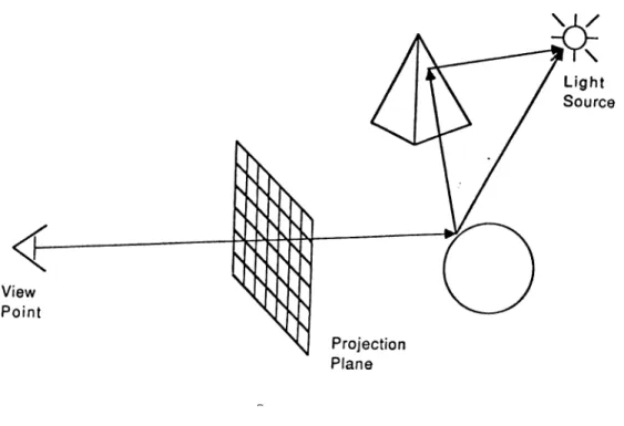
In a naive ray tracing algorithm, a ray is shot for each pixel from the view point into the three dimensional space as seen in Figure 2.1. Each object is tested to find the first surface point hit by the ray. The color intensity at the intersection point is computed and returned cis the value o f the corresponding pixel. In order to compute the color intensity at the intersection point, the ray is then refiected from this surface point to determine whether the reflected ray hits a surface point or a light source. If the reflected ray ends at a light source, highlights or bright spots are seen on this surface. If the reflected ray hits another surface o f an object, the color intensity at the new intersected point is also taken into account. This gives reflection o f a surface on another. When the object is transparent, the ray is divided into two components and each ray is traced individually.
As explained above, the color value at the intersection point gives the color value of the pixel associated with the intersecting ray. Therefore, having found the intersection point, the color at that point should be calculated according to a shading model. A simple one is given in the next section.
2.1
The Shading Model
2.1.1
Ambient Light
Initially the surface has ambient color which is a result o f the uniform ambient light emitted by the surrounding objects. That is, a surface can still be visible even if it is not exposed directly to any light source. In this case, the surface
Figure 2.1: Tracing o f one ray.
is illuminated by the objects in its vicinity. Ambient color behaves similarly regardless o f the viewing direction . We can express the intensity at a point on the surface o f an object as
Color„ = kdColova
where kd is the coefficient of reflection, Colora is the ambient light intensity.
kd takes values between 0 and 1. It is 1 for highly reflective surfaces. Unfor tunately, ambient color alone does not give satisfactory results. Therefore, the effect o f the light source(s) on the surface according to the orientation of the surface should also be considered in the computation of shading. That is, the diffuse reflections and the specular reflections add very much to the re alism o f the image. These computations use the reflection, normal and other vectors as seen in Figure 2.2. N is the unit vector normal to the point being shaded. L is the unit vector from the point to the light source. R is the unit vector in the reflection direction. The angle between R and N is equal to the angle between V and N. V is the unit vector from the viewing point to the point on the surface.
2.1.2
Diffuse Reflection
Diffuse reflection computation is based on the Lambert cosine law, which states that the intensity of the reflected light depends on the cosine of the angle between the normal of the surface and the ray to the light [33]. The cosine o f this angle is the dot product o f two unit vectors in the light and normal vector directions.
Diffuse reflection is computed as
kdColori
where Colorí is the intensity o f the light source, d represents the distance from a light source to the point being shaded and do is a constant to prevent denominator from approaching zero.
2.1.3
Specular Reflection
Highlights are seen from the view point when incidence light ray is at a certain angle and surface is shiny. The highlights (specular reflection) can be modeled as
where n is a constant related to the surface optical property. It is zero if the surface is dull and very large if the surface is a perfect mirror, fc, is a constant for speculcir reflection depending on the surface property.
2.1.4
Reflection
In order to simulate the reflection o f surrounding objects on the point being shaded, a reflection ray is sent from this point and this ray is tested with the objects to find any intersection. If this ray hits any object, the color intensity at the intersected point contributes to our shading computation as follows:
where Colorp was the intensity computed previously for the point being shaded. Color^ is the intensity at the intersection point, kr is a constant that is related to the surface property. It is coefficient o f reflection.
2.1.5
Transparency
If the shaded object is transparent, the reflections from the objects behind it should also be considered. This reflection contributes to the shading compu tation as
ColoTp = (1 — r)ColoTt + rColori,
Colort is the total intensity at the surface point after summing the intensities
o f the ambient light, the diffuse reflection and the specular reflection. Colors
is the intensity of the surface point behind the transparent object, r is a constant that is related to the transparency of the object. It is 0 if the object is opaque. In other words, the ray that hits a surface continues traveling through the transparent object until it intersects another object. The intensity at the intersection point is taken to contribute to the transparent object. This ray could also be refracted.
2.1.6
Shadows
Shadows that give very strong depth cues to the image can be obtained while finding out the diffuse and specular reflections. The regions o f a surface are in shadow if the light sources are blocked by any opaque or semi-transparent object in the scene. This is found out by sending a ray from the point on the surface towards the light sources and testing for intersection of the ray with an object before the light source. If there is any intersection both diffuse and specular reflections become zero.
3. SPEEDING UP THE ALGORITHM
As mentioned above, the major drawback which prevents ray tracing from being attractive for interactive systems is its computational complexity due to many intersection tests between rays and objects. Whitted has estimated that up to 95% o f the time is spent during these intersection tests [43]. They take too much time since all of the objects in the scene have to be tested to find the nearest intersection point with the ray, requiring intensive floating point operations. In order to reduce the processing time in the ray tracing algorithm, the computation for intersection tests should be decreased. There are two baisic approaches to do this. •
• First, an intersection test should be simple to compute. That is, it should take minimum number of computer cycles. The initial attempts to speed up the ray tracing were based on this approach. To make the intersection tests simple to compute, either intersection tests are made efficient [17,19,29,34,38,39] or bounding volumes explained in the next section are used.
• Second, the number of objects to be tested for intersections should be as few as possible. Not all of the objects in the scene should be tested for intersection with the traced ray as in the naive ray tracing algorithm. Only objects that are highly possible for intersection should be tested. In other words, the objects on the ray’s path should be considered for intersection tests. Several methods have been developed to achieve this. They are discussed in the next sections.
3.1
Bounding Volumes
Some simple mathematically defined objects such as spheres, rectangular boxes or cones can be tested for intersection with few number o f operations [13]. The complex objects are surrounded by these simple objects (bounding volumes) as in Figure 3.1 and intersections are first tested with the bound ing volumes instead of the complex objects . When the ray intersects the bounding volume o f an object, tests are carried out for the complex object as well. Obviously, the advantage o f using bounding volumes is to eliminate the intersection test with a complex object once its bounding volume is not intersected with the ray. Its disadvantage is the extra time spent in testing the bounding box if the object itself has a possible intersection. It should be noted that the bounding volumes are not mutually exclusive and thus a ray might be tested for an intersection with more than one object. This is another drawback o f the bounding volumes, since an intersection test for a complex object may take excessive time. When this type o f test is carried out more than once for a ray, it will be even worse.
When there is a large number o f objects in the scene, even the tests for
the bounding volumes can take an enormous amount o f time. By forming a hierarchy o f bounding volumes, a number o f tests can be avoided once a bounding volume that surrounds some other bounding volumes is not hit by the ray. Several neighboring objects form one level o f the hierarchy. The other drawback o f this method is that these hierarchies are diflicult to generate and manually generated ones can be poor. That is, they may not be helpful in speeding the intersection operation. Goldsmith has proposed methods for the evaluation of these hierarchies in approximate number o f intersection calculations required and for automatic generation o f good hierarchies [14].
The bounding volumes used can be spheres, rectangular boxes, polyhe drons, pгırallel slabs, cones, or surfaces o f revolution. The bounding volume chosen for each object in the scene can be different to enclose the object more tightly. This may be needed in order not to test more than one bounding volume for a ray.
3.2
Spatial Subdivision
A different approach to improve the efficiency o f ray tracing is called space subdivision [10,23]. The 3-D space that contains the objects is subdivided into disjoint rectangular boxes so that each box contains a small number o f objects. A ray travels through the 3-D space by means of these boxes. A ray that enters a box on its way is tested for intersection with only those objects in the box. If there eire more than one intersecting object, the nearest point is found and returned. If no object is hit, the ray moves to the next compartment (box) to find the nearest intersection there. This is repeated until em intersection point is found or the ray leaves the largest box that contains all o f the objects. It is necessary, in this case, to build an auxiliary data structure to store the disjoint volumes with the objects attached to them [36,37].
This preprocessing will require a considerable amount o f time and memory as a price for the speedup in the algorithm. It is, however, worth using the space subdivision particularly when the scene contains many objects, since
Figure 3.2: Adaptive space subdivision.
this data structure is constructed only once at the beginning eind is used during the ray tracing algorithm. The number of rays traced depends both on the resolution o f the generated image and the number o f objects in the scene. The auxiliary data structure helps to minimize the time complexity of the algorithm by considering only those objects on the ray’s way.
There are several techniques that utilize space coherence. They basically differ in the auxiliary data structures used in the subdivision process, and the manner used to pass from one volume to another.
In some ray tracing schemes that utilize the spatial coherence, the space subdivision process is based on the octree spatial representation. An octree is a hierarchical data structure organized such that each node cam point to one pzirent node and eight leaf nodes. Figure 3.2 shows this type o f subdivision o f the space. In the spatial subdivision ray tracing algorithm, each node of the octree corresponds to a region of the three dimensional space [11,12,14]. The octree building starts by finding a box that includes all o f the objects in the scene. A given box is subdivided into eight equally sized boxes according to a subdivision criterion. These boxes are disjoint and do not overlap as the bounding volumes might do. Each of the generated boxes are examined to
Figure 3.3: Subdivision o f space into equtilly sized cubes.
find which objects o f the parent node гıre included by each child node. The child nodes are subdivided if the subdivision criterion is satisfied. This is carried out recursively for each generated box.
The subdivision criteria may be based on the number of objects in the box, the size o f the box, the density ratio o f total volume that is enclosed by all objects in the scene to the volume of the box. When the criterion for the number o f objects in a given box is very large, each object in the scene is tested for intersection for all rays as in the naive algorithm. No speedup will be achieved, on the contrary the time and the memory will be wasted for the octree data structure. On the other hand, if the number o f objects is one for the criterion, there will be many boxes in the structure and the overhead for traveling through the 3-D space may increase.
Kaplan used a data structure which he calls BSP (Binary Space Partition ing) tree to decompose the three-dimensional space into rectangular regions dynamically [23]. BSP is very similar to octree structure in that it also di vides the space adaptively. The information is stored as a binary tree ( a tree where each non-terminal node can have exactly two child nodes) whose non-leaf nodes are called slicing nodes, and whose leaf nodes are called box
nodes and termination nodes. Each slicing node contains the identification o f a slicing plane, which divides all o f space into two infinite subspaces. The slicing planes axe always aligned with two o f the cartesian coordinate axes of the space that contains the objects. The child nodes o f a slicing node can be either other slicing, termination nodes or box nodes. A termination node denotes a subspace which is out o f the three-dimensional space that does not contain any objects. A box node , on the other hand, is described by the slic ing nodes that are traversed to reach it. They denote a subspace containing at least one object. BSP actually encodes the octree in the form o f a binary space partitioning tree and it is traversed to find the node containing a given point.
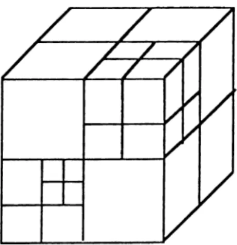
The other spatial subdivision technique for ray tracing is based on the decomposition o f the 3-D space into equally sized cubes [10]. Figure 3.3 contains a scene decomposed into equally sized volumes. The size o f the cubes determines the number o f objects in each cube. Therefore, zin optimal cube size must be considered such that the overhead for moving through the boxes should not exceed the time gained in testing intersections.
Fujimoto proposed a scheme that imposes an auxiliary structure called SEADS (Spatially Enumerated Auxiliary Data Structure) on objects in the scene [10]. This structure uses a high level of object coherency. He also developed a traversing tool that fits in well with SEADS to t2ike advan tage o f the coherency in a very efficient way based on incremental integer logic. This method, called 3DDDA (3-D Digital Differential Aneilyzer), is a three-dimensional form o f the two-dimensional digital-differential analyzer algorithm commonly used for line drawing in raster graphics system. The major advantage o f this scheme is related to the manner to travel through 3-D space containing the objects. 3DDDA does not require floating-point multiplications or divisions in order to pass from one subspace (voxel) to the next while looking for intersections, once a preprocessing for the ray has been performed. Fujimoto states that an order o f magnitude improvement in ray tracking speed over the octree methods has been achieved. It is also possi ble to improve the performance of octree traversal by utilizing the 3DDDA method to traverse horizontally in the octree, but vertical level changes must
be traversed as usual.
3.3
A Hybrid Technique
Recently, Glassner has presented techniques for ray tracing o f animated scenes efficiently [13]. In his technique, he renders static 4-D objects in spacetime instead o f rendering dynamically moving 3-D objects in space. He uses 4- dimensional analogues familiar to 3-dimensional ray-tracing techniques. Ad ditionally, he performs a hybrid adaptive space subdivision and bounding volume technique for generating good, non-overlapping hierarchies o f bound ing volumes. The quality o f the hierarchy and its non-overlapping property is an advantage over the previous algorithms, because it reduces the number o f ray-object intersections that must be computed.
The procedure to create such a hierarchy starts by finding a box that encloses all o f the objects in the scene, including light sources and the view point. The algorithm then subdivides the space adaptively as in the octree method. The subdivision that is based on a given criterion is performed for each box recursively. The recursion is terminated when no boxes need to be subdivided.
As returning from the recursive calls made by the space subdivision pro cess, the bounding volume hierarchy is constructed. Each box is examined, and a bounding volume is defined that encloses aill the objects included within that box. The defined bounding volume must not intersect any other box. That is, it is clipped by the space subdivision box.
At the end o f this process, a tree o f bounding volumes that has both the nonoverlapping hierarchy o f the space subdivision technique and the tight bounds o f the bounding volume technique is constructed. Thus, the new hierarchy has the advantages o f both approaches while avoiding their draw backs.
3.4
Parallel Ray Tracing
One other approach that is useful to speed up the algorithm is to use several processing elements running in parallel. Since the rays are traced indepen dency from each other, the eilgorithm can be easily parallelized by distribut ing the computation related to different rays.
The simplest way to parallelize the algorithm is to partition the image space into several rectangular regions and to compute pixel values for each disjoint region in parallel. The image can be partitioned in several ways: the regions may be obtained by simply dividing the image space into equal sized rectangles. Each rectangular area is computed on different processing elements and the generated images are joined as a single image. A disadvan tage of dividing the image space in this way is related to the distribution of computation load to different processing elements unevenly. That is, some processing elements may complete their tasks much earlier than others, since less objects are contained in the viewing volume associated with the region. The other approach to obtain the subimages divides the image space adap tively in order to distribute the tasks evenly. The subimages obtained in this way may be of different sizes but they should require approximately the same computation time so that no processing element is idle for a long time, while others are busy. In this case, we may achieve a speedup that is close to the number of processing elements running in parallel.
Another parallel ray tracing is essentially based on the spatial subdivision mentioned eeirlier [9]. The 3-D space containing the objects is subdivided into several disjoint volumes. The computation in each volume is carried out on a different processing element. The ray that travels through 3-D space to find an intersection passes from one processing element to another via messages. Each processing element contains the information about the volume assigned to it. A suitable architecture to accomplish this can be three dimensional array processor. In this architecture, each processing element is connected to 6 neighboring processing elements in order to pass messages which consist o f information about the rays. On the other hand, hypercube architecture has potential to perform this task as 3-D array processor. A hypercube of
dimension d contains 2** processors [35]. Assume the processors are labeled 0,1,...,2*^ — 1. Two processors i and j are directly connected iff the binary representations o f i and j differ in exactly one bit. Its advantages in this context may come from its recursive definition and embedding the 3-D array processor architecture.
Both o f the above ideas can be combined to reach at a more efficient utilization o f processing elements [6,9,30]. The 3-D space is again decomposed into disjoint volumes which are assigned to different processing elements. In this case, several rays are traced independently in peirallel by subdividing the image space as well. A more detailed parallel ray tracing can be seen in [6,9].
Miiller has attempted to ray trace movies by distributing the frames to different Workstations connected through a network [26]. They generated a 5-minutes ray traced animation within 2 months without boring the users of the Workstations by efficiently using the network.
4. AN IMPLEMENTATION OF SPACE
SUBDIVISION USING OCTREE
4.1
Overview
The space subdivision method can be broken up into two different steps; preprocessing and ray casting. We first build an auxiliary data structure that will be then used while traveling through the 3-D space. The auxiliary data structure will contain the information that will allow ray-environment intersections to be computed as quickly as possible. The 3-D space which contains all o f the objects in the scene is divided into a hierarchical structure o f cubic boxes aligned with the cartesian coordinate system. In the algorithm that uses space coherence, the only difference is in the intersection routine to find the first object hit by the ray, if there is any. The new intersection routine will be as follows: •
• Find a point along a given ray in the first box it intersects. If the ray is originated inside the root box that encloses all o f the boxes, the starting position is the point looked for. Otherwise, the ray that is originated outside the root is tested for intersection with this largest box. The point to be returned is the one a little further from the intersection point which is in the first box on the path o f the ray. If the ray does not hit the root box, the next ray is shut from the viewpoint and no intersecting object is returned.
• Having found a point, find the box id that is associated with that point. This step may take most of the time for traveling through the boxes.
Therefore, the data structure should be designed so that we can access a box in the hierarchy for a given box name quickly.
• At this step, only the objects in the currently visited box are tested for intersection. Since each box contains few number o f objects, we spent a little and approximately constzint time in each box. If the ray hits more than one object in the same box, the nearest intersection point is returned. If the ray does not hit any object in this box, we move to the next box along the ray and perform intersection tests with the objects in this box. This process is repeated until an intersection is found or the ray leaves the root box.
Basically, there are three operations to be performed for the above algorithm. They are:
• Given a point in space, find the box and its data. Since space is divided dynamically eind unevenly, this cannot be performed simply by indexing into a three-dimensional table o f box references.
• Given a ray that originates within a given box, find the next intersected box, if there is. Otherwise, return a message signaling that it will leave the largest box.
• Given a box that describes a subspace of the scene, obtain a list of all objects whose surfaces intersect that box. Only the objects in this list will be tested for intersection with each ray that passes through the box.
The new algorithm after subdividing the 3-D space into cubic boxes will refer to the data base frequently. Therefore, it is important for the sake of the speed to organize the data structure so that it will be easy to access the information contained in it. We used a hierarchical data structure called octree to store this information. Octree structure consists o f nodes that represent a subspace of the scene. A node is a leaf node if it is not subdivided any more. Each non-leaf node has eight children each of which describe a subspace of the parent node. The volumes described by children nodes are
! 5 I 1 5 2
1 5 3 1 5 4
158
Figure 4.1: Naming the boxes.
disjoint and are equal in size. The root node which encloses all of the objects in the scene is labeled node 1. When we subdivide a node, it passes its name as a prefix to all its children, which are numbered 1 through 8, as shown in Figure 4.1. Thus the eight children of the root node are nodes 11 through 18. The children o f node 15 are nodes 151 through 158, and so on. Now, we should answer the second question in the previous section. That is, how could we find the address of the box given its label ?
We can accomplish this in two extreme ways. In the first way, we could build a table with an entry for every possible node name that contains that node’s address. Obviously, this possibility will require large amount o f mem ory. This is due to the fact that not all possible nodes need to be created. Instead, the nodes o f octree are created dynamically when needed. If we subdivide the root node twice, the maximum possible box name is 188. For example, we may not need to create nodes 151-158 if node 15 does not satisfy a subdivision criteria. On the other hand, this scheme would have the advan tage o f extreme speed in finding the address of a node for a given name. In the second way, we could construct the hierardiy by using linked lists. This time, each node would have eight pointers to its children and each time we would search the tree from beginning to find a node address o f a given node
name. This scheme requires less memory than the first one but searching for a node slows down the operation and may come up with great overhead.
4.2 Octree Building and Storage
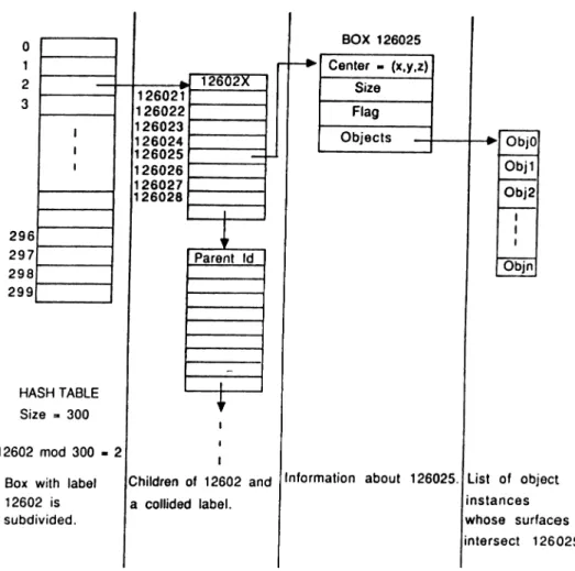
We mixed these two methods using a hashing scheme in the same way as Glassner did [12]. In this scheme, we have a hash table to hold pointers to a structure. This structure contains addresses o f eight children o f a subdi vided node and the name of their parent node as shown in Figure 4.2. The construction o f the data structure is as follows:
1. Find a cubic box, called root, which contains all o f the objects in the scene. A box is defined by its center, size, a flag and a list of objects whose surfaces intersects with this box. Flag is set to zero for a leaf box.
2. If the root box contains objects more than a specified number, go to the next step to subdivide it into disjoint volumes. Otherwise, this is the leaf node. No further actions are to be taken for this box.
3. Using the name o f current box that is to be subdivided, compute a hash function. We use a very simple hash function which is the node name modulo tablesize. Let in d e x be the computed hash function.
4. The in d e x is the location where we want to put the consecutive ad dresses o f eight children and their parent name. If this location is not empty, the collided node names form a linked list. That is, by simply following the linked list, the new structure is appended to the end of this list. If this location does not point to any structure, it will contain the address o f the new structure.
5. Now, for each generated child, find the center and the objects the sur faces o f which intersect the box represented by the child. The size of the child node is the half o f the parent’s size.While determining the sizes of generated boxes, the minimum size of the boxes is stored in a
Figure 4.2: Heish table to store the generated boxes.
global variable ceilled M in len . M in le n is to be used later for moving from a box to another.
6. If the number o f objects pointed by a child exceed a specified value, Its flag is set to a non-zero value. Each child node is subdivided as its parent if the flag is non-zero. That is, we go to the step 3 for each child with a non-zero flag.
4.3
Movement to the Next Box
Whenever no object in a box intersects the ray being traced, the next box, if any, on the ray’s path should be determined and this time the intersection tests are ceirried out with the objects in this box. Movement to the next box continues until an intersection point is found, or until the ray leaves the root box. There are two issues involved in this operation: First, because the space is dynamically decomposed when we build the octree, we do not know how large (or small) any box in space is with the exception o f the current one. That is, how far should we move in order to guarantee that we are in the next box, but not in another. Secondly, movement to the next box should be fast enough so that we do not loose what we gain by decomposing the 3-D space into boxes.
The essence of the box-movement algorithm is to find a point that is guaranteed to be in the next box whatever its size. This point is then used to derive a box name and the address o f this box along with the information contained in it.
A point on a ray can be defined by a parameter t. The value o f t increases as we move away from the origin, where t has the value 0. The parametric line equations give us the point P = (x, y, z) corresponding to parameter t
as below:
X = Xa + tX r
y = y, + ttjr
Z = Za + tZr
where (x ,,j/a ,z ,) is the starting position o f the ray, (xr,yr,Zr) is the move ment in each direction. Given a box definition and a ray that passes through the box, we can find the maximum value of t which may attain in this box. Let this parameter be tmax which will give the intersection point when the ray leaves the box. We can compute tmax by intersecting the ray with the six planes that bound the current box. Two of these intersections give us bounds on t for X —planes, two others for y —planes and the remaining two for
z —planes. Since each plane is parallel to two o f the three coordinate axes.
it is inexpensive to intersect a ray with one of these ’’ simple” planes. Let the bounds be denoted by tXminytXmax^iyminjiymaxy^^mim^^max· For exam ple,
tXmin
is the minimum, tx^ax is the maximum o ft
values that give the intersection points with x —planes. The other four are used similarly. Note that the points describing the intersections of the ray with the planes o f the box may lie far outside the value o f the box itself. But certainly some values o ft
will hold for all three ranges: these are the values o ft
inside the box. The intersection o f three ranges {tXmin--t^max,tymin-tymax,tZmin-tZmax) gives the values oft
that the ray may take while it is inside the box. The value ofiffidx IS the minimum o f iXmax^ "^ymax snd i^nuix·
Now, we will use the variable M in len to find a point in the next box. M in le n was the size o f the smallest box. Having found the parameter tmax,
we compute P = ( x , y , z ) using above equation We find the point within the next box along the ray by merely moving perpendicularly to the planes by a distance M in le n if their
t
values are equal totmax·
H the point of intersection is on an edge, that is, when two of the parameters are equal totmax,
we must travel perpendicularly to both faces sharing that edge, and similarly we must travel in three directions if tmax is on a corner o f the box. We simply increment x ,y or z component o f the point P by M in len , if the corresponding t value is equal totmax·
Now, using this point, we should access the box and its information. We start by checking whether the point is in root or not. If the point is outside the root box, we return and report this. If it is in the root box that has label 1, we find the children o f the root box by using the hash function. Next, we can decide which one of eight children contains this point. The same process is applied recursively for the child node that includes that point until a box that has a zero flag is reached. Flag was set to zero for the leaf boxes.
5. A RAY TRACER SYSTEM
A ray tracing system is designed and implemented in C programming lan guage [24] on SUN^ Workstations running under UNIX^ operating system. The system has three major parts:
• Create a scene with objects provided by the system.
• Process the defined scene to obtain a realistic image that consists of RGB values.
• Display the generated image.
The system mainly can be used to create scenes containing 3-D objects and then find out the effect o f light sources and the objects on each other. Each part is to be explained in detail in the following sections :
5.1
Defining the Scene
This is the first step in generating a realistic image. User is provided with several types of objects to model the scene. In addition to the definition of objects to be included in the scene, the user can give a number o f parameters such as point light sources, viewpoint, origin of the scene etc. so that the processing is carried out with these parameters, otherwise, which would be assigned default values. The mentioned input can be given in two different ways :
^SUN Workstation is a registered trademark of Sun Microsystems, Incorporated. ^UNIX is a registered trademark of AT&T Bell Laboratories.
• A text file can be prepared with definitions o f objects and scene param eters using a text editor.
• The scene can be defined using an interactive tool that gives a friendly environment to the user.
5.1.1
Textual Input
When a person chooses the first way to define a scene, he must describe the scene according to a given syntax. UNIX tools LEX and YACC have been used to parse and process the user input [41]. The file consists o f three kinds o f information :
• Scene Parameters, • Object Definitions, • Material Properties.
S ce n e P a ra m e te rs
Scene parameters are related to the things in the scene other than the objects. Each parameter declaration is started by a keyword that consists o f uppercase letters. A set of values follows this keyword. The parameter declarations are given in the following form :
V I E W P O I N T X y z
This is the place in three-dimensional space where the eye o f the observer is located.
O R I G I N X y z
This is the point in three-dimensional space where the eye looks at.
U P V E C T O R X
y
ZThis is used to describe the orientation o f the user, (a;, y, z) is a normal vector that indicates the viewing direction.
R A S T E R w i d t h h e i g h t
It is the resolution o f the screen, ’’ width” and ’’ height” are the size o f the screen in terms o f number of pixels.
V I E W P O R T w i d t h h e i g h t
This gives the window size that the user can see.
R D E P T H n
This is used for the termination condition o f the recursive call to the shad ing routine. It actually gives interreflections between objects. If n is 0, no reflections exist on the objects.
I M A G E F I L E f i l e n a m e
The computed RGB values are written on the given file name.
L I G H T b r i g h t n e s s
X y z
This is to define a point light source anywhere in the three-dimensional space, ’’ brightness” gives the intensity o f the point light source and ranges from 0 to 1. It is 0 if no illumination is done by the source. Next triple gives the position o f the point light source.
Object Definitions
Next comes the definition o f objects in the scene. There are five types of objects definable by the system. They axe sphere, superquadric, triangle, rectangle and box. Their textual descriptions are as follows :
Each object description is started by a keyword followed by a surface number and the parameters to define the object. Surface number is an integer that refers to a surface definition used for shading computations.
Sphere has two parameters which are center and radius o f the sphere.
S P H E R E s u r f a c e - n u m b e r
r a d i u s
X y z / ♦ c e n t e r o f t h e s p h e r e * /
Note that comments can be written as in the C language to make the description more understandable.
A box can be defined by its center and the size information from the center. Boxes are always aligned with the coordinate axes.
B O X s u r f a c e - n u m b e r
x c y c z c / ♦ c e n t e r o f t h e b o x * /
x s y s z s / * s i z e o f t h e b o x * /
Superquadrics in the context o f this system can be defined as boxes whose corners are rounded. Therefore, a superquadric is defined similarly to a box with an additional parameter called ’’ Power” . ’’ Power” gives the degree of roundness o f the corners. Its definition is as follows :
S U P E R Q U A D R I C s u r f a c e - n u m b e r
p o w e r
x c y c z c / * c e n t e r o f t h e s u p e r q u a d r i c ♦ /
x s y s z s / * s i z e a s i n b o x d e f i n i t i o n ♦ /
A triangle in three dimensional space is defined by its three corners, the points o f the corners should be given in the counterclockwise direction that is very important in shading computations. The syntax for a triangle decla ration is : T R I A N G L E x l y l z l x 2 y 2 z 2 x 3 y 3 z 3 s u r f a c e - n u m b e r
Similar to a triangle definition, a rectangle is defined by its corners. Again, the corners should be given in counterclockwise direction. Its syntax is :
R E C T A N G L E x l y l z l x 2 y 2 z 2 x 3 y 3 z 3 x 4 y 4 z 4 s u r f a c e - n u m b e r
Material Properties
A surface description that is referred by the objects serves the shading com putations in all steps. A surface description can be given as follows :
S U R F A C E s u r f a c e - n u m b e r r l g l b l / * a m b i e n t c o l o r ♦ / r 2 g 2 b 2 / * d i f f u s e r e f l e c t i o n * / r 3 g 3 b 3 / * s p e c u l a r r e f l e c t i o n ♦ / k / * c o n s t a i n t r e l a t e d t o t h e s u r f a c e p r o p e r t y * / r / * r e f l e c t i v i t y c o e f f i c i e n t * / t / * t r a n s p a r e n c y c o e f f i c i e n t ♦ / 29
5.1.2
Interactive Tool
The other way to specify a scene is to use an interactive tool. The user can give the description o f a scene using mouse, menus etc. in a user friendly environment. This tool projects the three-dimensional world onto the two- dimensional screen to provide user with an easy user interface when entering three-dimensional points.
Using this tool, the scene description mainly involves selecting one of the object types and specifying the size and other parameters related to the selected object type by the mouse, panel and other windowing system elements. A more detailed information on the interactive tool is given in the appendix as the user’s manual.
After completing the description o f the scene, the system converts it into the format given in the previous section and writes the textual description on a text file. Therefore, this interactive tool is nothing but a shell that generates the description on a text file as an output. The textual description o f a scene is useful in the sense that the ray tracer can be portable to any computer system.
B-Spline Surfaces
The other advantage of the interactive tool is that user can generate free form surfaces other than five primitive object types. A free-form surface can be created and placed into 2in appropriate location in the scene. B-Spline method is used by the system to find out the surface to be included in the scene description. The surface generated is then triangulized and written in the known format on the output file as a collection o f triangle primitives.
Since objects with complex shapes occur frequently in our three-dimensional world, special techniques to model them properly are needed [31]. Although these objects can be approximated with arbitrarily fine precision as plane faced polyhedra, such representations are bulky and intractable. For example, a polyhedral approximation o f a hat might contain 1000 faces and would be
difficult to generate and to modify. We need a more direct representation of shapes, easy both to the computer and to the person trying to manipulate the shapes. Bézier and B-Spline are the two methods frequently used to generate curves and surfaces o f 3-D. They are similar to each other in that a set of blending functions is used to combine the effects o f the control points. The key difference lies in the formulation o f the blending functions [3,18,31].
5.2
Processing: Ray Tracer
This part accepts a textual scene description as input that was explained in the previous section and it generates an image containing several optical effects for the sake o f realism using ray tracing zilgorithm. There are three m ajor data structures used by this module. They are used to store the objects, the surfaces and the light point light sources in the scene. The objects are stored in an array that has elements o f the following structure:
O B J E C T T Y P E
O B J E C T I D
S U R F A C E NUMBER
P O I N T E R TO AN O B J E C T I N S T A N C E
OBJECT T Y P E indicates one o f the five primitive objects. For example, O BJECT T Y P E for a sphere is 0. It is iise.d to call intersection and nor mal routines related to OBJECT TYPE. OBJECT ID indicates the object instance in the scene. It is used to access the object variables in intersec tion and normal routines. SURFACE NUMBER refers to a surface definition that gives the object material property. The last entry is an address to an object instance. For example, the address in this entry may contain a sphere definition as below:
R A D I U S
X Y Z
The surface definition are stored in an array o f the following structure:
A R AG AB / ♦ A m b i e n t c o l o r c o m p o n e n t s * / DR DG DB / ♦ D i f f u s e c o l o r c o m p o n e n t s * / S R SG S B / * S p e c u l a r c o l o r c o m p o n e n t s * / C O EF / * S u r f a c e c o e f f i c i e n t ♦ / R E F L / * R e f l e c t i o n c o e f f i c i e n t * / T R A N S P / * T r a u i s p a r e n c y c o e f f i c i e n t * /
Point light sources are simply stored in an array o f lights. Each light is defined by
B R I G H T N E S S
X Y Z
Each object type definable by the system has its own intersection function. This gives a great flexibility for adding new objects to the system. That is, if a new object type is to be added to the system , the following should be available for the new object type:
• Object Definition
• A function that allocates space for an instance o f the new object type. • A function that finds out the intersection point on the surface with a
ray. This is used during intersection tests.
• A function that returns the normal vector at a given point on the object surface. This is used for shading computations.
Additionally, the intersection calculations become more efficient since each function is implemented for a specific object type.
The shading model used by the system is similar to the one given in the second chapter. Ambient color that is stored in surface definition is the initial color for the point being shaded. The diffuse and specular reflections are calculated by using the entries in the surface structure. The level of reflection is the terminating criterion for the recursive call when the reflected
ray hits another object other than light source. Transparency o f an object is simulated by the given calculation model. That is, the ray is divided into two components and one o f them continues traveling through the treinsparent object until it hits another object at its back. After calculating the intensity at the hit point, the intensity at the point o f the transparent object is found out by the given formula. In addition to these optical effects, shadows that give very strong depth cues may exist if the light is blocked by opaque or semi-transparent objects.
This part o f the system has three different versions. The first version of the system is based on the naive ray tracing algorithm. That is, all objects in the scene are tested to find the first intersection with a traced ray. As it is very obvious, the time spent increases with the number o f objects in the scene. For example, when we have 10,000 objects in the scene, processing may take even days on a mini computer.
In the second version o f the ray tracing system, the intersection tests are not carried out with all objects in the scene but the spatial coherence technique is used to perform intersection tests only for the objects that are on the path o f the ray. Therefore, the space containing the objects is subdivided using the octree representation. The second version o f the program is capable o f generating the images much faster than the first version that does not utilize the space coherence.
The last version is the parallel ray tracing algorithm. It partitions the image space into four equal sized rectangles and generates pixel values for each o f them on a different file. It is just a simulation o f the parallel algorithm using UNIX’s ’’ fork” and ’’ wait” system calls [42]. No actual speedup is achieved, since only one processor is used.
5.3
Displaying the Image
We compute a triple (R G B ) for each pixel o f the image after tracing a ray. When we compute RGB values in shading routine, we assume a linear inten sity response. That is, pixel o f a value o f 127, 127, 127 has the half intensity
o f a pixel value o f 255, 255, 255. However, the response o f typiczil video color monitors and o f the human visual system is non-linear. Thus, displaying of images in a linear format results in effective intensity quantization at a much lower resolution than the available 256 resolution per color. That is, the true colors will not be perceived by the human eye, because o f the non-linearity in the monitor. Therefore, it is necessary to correct the computed values so that the generated picture appears more realistic to a human observer.
A function called gamma correction is used for this purpose [16]. It is an exponential function o f the form:
lookupvalue —
Gamma represents the nonlinearity o f the monitor. Generally monitors have a gamma value that is in the range 2.0 to 3.0. If gamma is equal to 1, the device is a linear one. An incorrect value results in incorrect image contrast and chromaticity shifts. If the gamma is too small, the contraist is increased and the colors approach to the primaries.
The RGB values should be corrected by the above function before the image is displayed or stored to a file.
5.4
Examples and Timing Results
In this section, several images generated by our system are presented in Fig ures 5.1, 5.2, 5.3, 5.4, 5.5, 5.6, 5.7, 5.8. We also compare the time spent in the first and second version o f the algorithm for some images.
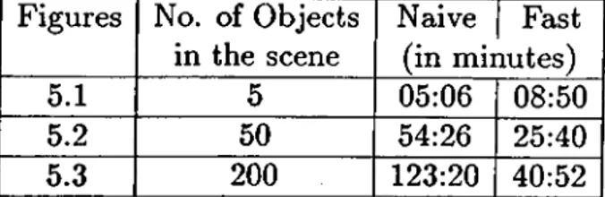
Table 1 contains the clock timings for rendering three images given in Figures 5.1, 5.2, 5.3. Actually, there may be several other influences on the rendering time other than the complexity o f the algorithm. These are the programming style, the code optimization, the processor speed, etc. As it is clear from these measurements, when the number o f objects in the scene in creases, the ratio o f the naive technique to the fast one gets larger and larger. This is due to the fact that a great amount o f time is wasted for the inter section calculations in the naive ray tracing system. The ratio approaches
Figures No. o f Objects in the scene Naive 1 Fast (in minutes) 5.1 5 05:06 08:50 5.2 50 "54:26 25:40 5.3 200 123:20 40:52
Table 5.1: Timing results o f figures 5.1, 5.2, 5.3.
No. o f Objects in boxes Time (in minutes) 2 22:21 6 17:52 8 28:36
Table 5.2: Timing results of figure 5.4.
one for the scenes containing few number of objects [21]. In higher speed models, we note that the timings are dependent on the criteria used to subdivide the space. For example, when the space is divided into very small boxes that contain only one object, the overhead for traveling through the boxes may approach to the time saved for intersection tests. That is, the ray may frequently pass through many empty volumes wasting a considerable amount o f time. Table 2 shows timings for the image in Figure 5.4 gener ated using the octree auxiliary data structure for three different terminating criteria values.
Figure 5.1: Four spheres and a triangle.
F ig u r e 5 .2 : F ift y sph eres.
Figure 5.3: Two hundred spheres.
§
i
F ig u re 5.4: T w e n ty fo u r sph eres.
Figure 5.5; Sphere above chessboard.
F ig u re 5.6: S h ield a n d a sp h ere.
Figure 5.7: Boxes and superquadrics.
F ig u r e 5.8: M irro rs a n d re fle ctio n s.
6. CONCLUSICN
Computer generated images that appear realistic to a human observer have been one o f the most important goals in Computer Graphics. Ray tracing algorithm with this respect is the most popular method for realistic image synthesis. It is in the class o f image generation algorithms, called global shading, that provide the most realistic images by considering the optical effects such as shadowing and reflection from the surfaces in the environ ment. However, it requires a tremendous amount of time to generate an image. Several methods have been developed to overcome the time problem [6,9,10,11,12,13,23,28,29]. In this thesis, we investigated these methods and used two o f them, namely space subdivision and parallelism, in the imple mentation o f the ray tracing system. The space subdivision method saves considerable amount o f time when the scene is complex. Hut the speedup achieved is still not enough when many images are to be generated. The parallel version o f the space subdivision method may be the best solution for the time problem. As the first conclusion, the parallelism is essential for the interactive realistic image generation.
Another method in the global shading class has been introduced later than ray tracing as radiosity [7,15,20]. This method can simulate the global illumination effect more accurately than ray tracing can do. Although there has been several attempts to obtain more detailed images using ray tracing as in [1,5,8,22], no one could consider the interaction between diffuse surfaces. Another advantage o f radiosity method is that the resultant surface intensities are independent o f the viewer position. This allows efficient rendering of dynamic sequences. As the next conclusion, ray tracing should utilize some ideas in this method, namely radiosity to increase the accuracy in simulating
the global illumination effects.
Finally, we should also taJce into account the texture mapping that is used to cover over a surface with texture [4], in order to provide more detailed im ages. Texture mapping is basically the method of wallpapering the polygons in the scene. One o f the future directions in realistic image generation is to develop methods for ray tracing texture mapped surfaces in a reasonable ajnount o f time.