An improved spring embedder layout algorithm for compound graphs

AN IMPROVED SPRING EMBEDDER

LAYOUT ALGORITHM FOR COMPOUND

GRAPHS

a thesis

submitted to the department of computer engineering

and the graduate school of engineering and science

of bilkent university

in partial fulfillment of the requirements

for the degree of

master of science

By

Alper Kara¸celik

August, 2012

I certify that I have read this thesis and that in my opinion it is fully adequate, in scope and in quality, as a thesis for the degree of Master of Science.

Assoc. Prof. Dr. U˘gur Do˘grus¨oz(Advisor)

I certify that I have read this thesis and that in my opinion it is fully adequate, in scope and in quality, as a thesis for the degree of Master of Science.

Assist. Prof. Dr. Burkay Gen¸c

I certify that I have read this thesis and that in my opinion it is fully adequate, in scope and in quality, as a thesis for the degree of Master of Science.

Dr. Cevat S¸ener

Approved for the Graduate School of Engineering and Science:

Prof. Dr. Levent Onural Director of the Graduate School

ABSTRACT

AN IMPROVED SPRING EMBEDDER LAYOUT

ALGORITHM FOR COMPOUND GRAPHS

Alper Kara¸celik

M.S. in Computer Engineering

Supervisor: Assoc. Prof. Dr. U˘gur Do˘grus¨oz August, 2012

Interactive graph editing plays an important role in information visualization systems. For qualified analysis of the given data, an automated layout calculation is needed. There have been numerous results published about automatic layout of simple graphs, where the vertices are depicted as points in a 2D or 3D plane and edges as straight lines connecting those points. But simple graphs are insufficient to cover most real life information. Relational information is often clustered or hierarchically organized into groups or nested structures. Compound spring embedder (CoSE) of Chisio project is a layout algorithm based on a force-directed layout scheme for undirected, non-uniform node sized compound graphs.

In order to satisfy the end-user, layout calculation process has to finish fast, and the resulting layout should be eye pleasing. Therefore, several methods were developed for improving both running time and the visual quality of the layout. With the purpose of improving the visual quality of CoSE, we adapted a multi-level scaling strategy. For improving the performance of the CoSE, the grid-variant algorithm proposed by Fruchterman and Reingold and parallel force calculation strategy by using graphics processing unit (GPU) were also adopted. Additionally, tuning of the parameters like spring constant and cooling factor were considered, as they affect the behavior of the physical system dramatically. Our experiments show that after some tuning and adaptation of the methods above, running time decreased and the visual quality of the layout improved significantly.

Keywords: Interactive graph editing, Automated graph layout, Force-directed placement, Compound graph, FR-Grid Variant, Multi-level scaling, Parallel pro-gramming.

¨

OZET

˙IY˙ILES¸T˙IR˙ILM˙IS¸ B˙IR B˙ILES¸˙IK C¸˙IZGE YERLES¸T˙IRME

ALGOR˙ITMASI

Alper Kara¸celik

Bilgisayar M¨uhendisli˘gi, Y¨uksek Lisans Tez Y¨oneticisi: Do¸cent Dr. U˘gur Do˘grus¨oz

A˘gustos, 2012

Etkile¸simli ¸cizge d¨uzenleme, bilgi g¨orselle¸stirme sistemlerinde ¨onemli bir rol oy-namaktadır. Eldeki verinin kaliteli analizini yapmak i¸cin otomatikle¸stirilmi¸s yerle¸sim hesaplaması yapmak gerekmektedir. Basit ¸cizgelerin otomatik yerle¸siminin yapılmasına ili¸skin bir ¸cok ¸calı¸sma yapılmı¸stır. Genellikle bu basit ¸cizgelerde k¨o¸seler iki ya da ¨u¸c boyutlu d¨uzlemde nokta, kenarlar da bu nokta-ları ba˘glayan do˘gru ya da e˘griler olarak g¨osterilmektedir. Ancak, ili¸skisel veriler, genellikle hiyerar¸sik veya k¨umelenmi¸s olarak organize edilmektedirler. CoSE ile, kuvvet y¨onelimli yerle¸sim ¸semasına dayalı bir bile¸sik ¸cizge yerle¸stirme algoritması sunulmaktadır. CoSE ile birlikte y¨ons¨uz, birbirinden farklı b¨uy¨ukl¨ukte k¨o¸selere sahip bile¸sik ¸cizgelerin yerle¸simi sa˘glanmaktadır.

Kullanıcı memnuniyetini sa˘glamak i¸cin ¸cizge yerle¸stirme i¸sinin kısa s¨urede tamamlanması ve ¸cizgenin g¨oze ho¸s gelen bir bi¸cimde ekranda yer alması gerek-metedir. Hem performans hem de g¨orsel kalitenin iyile¸strilmesi amacıyla sunulan bir ¸cok method bulunmaktadır. Bu tez ¸calı¸smasında CoSE’nin g¨orsel kalitesinin geli¸stirilmesi amacıyla ¸cok seviyeli ¨ol¸ceklendirme stratejisini adapte ettik. Ayrıca, ¸calı¸sma zamanının iyile¸stirilmesi i¸cin de Fruchterman ve Reingold’un kareleme y¨ontemi ile grafik i¸sleme unitesi (GPU) ¨uzerinde e¸s-zamanlı programlama strate-jisini CoSE’ye uyguladık. Ek olarak, yay sabiti, serinleme fakt¨or¨u ve benzeri parametrelerin ayarlanması i¸sini de fiziksel sistemin davranı¸sını ¨onemli ¨ol¸c¨ude etk-iledi˘gi i¸cin dikkate aldık. Yaptı˘gımız deneyler g¨osterdi ki, parametre ayarlamaları ve yukarıda bahsedilen metodların adaptasyonu ile birlikte CoSE algoritmasının ¸calı¸sma s¨uresi ¨onemli ¨ol¸c¨ude azalırken, sonu¸c ¸cizgelerin g¨orsel kalitesi ise ¨onemli miktarda iyile¸stirildi.

v

Anahtar s¨ozc¨ukler : Etkile¸simli ¸cizge d¨uzenleme, Otomatik ¸cizge yerle¸simi, Kuvvet y¨onelimli yerle¸sim, Bile¸sik ¸cizge, FR kareleme y¨ontemi, C¸ ok-seviyeli ¨

Acknowledgement

First and foremost, I would like to thank to my advisor, Assoc. Prof. U˘gur Do˘grus¨oz for his guidance and patience during my thesis study. He always in-spired me for pushing myself harder and motivated me for finding the best solu-tions all the time.

I would also like to thank to the authority of Bilkent University for providing me with a good environment and facilities to complete my thesis. I am very grateful to all the instructors that helped me to improve my academic knowledge. During the two years, I have shared my office with fun and friendly colleagues. Thanks to them, I always felt like at home. But my special thanks are to one of my best friends, Sel¸cuk Onur S¨umer. My graduate period would not be the same without him. Also, I would like to thank to Salim Arslan for his assistance during my graduation.

Finally, yet most importantly, I would like to thank my parents with all my heart for their endless love and support and to my friends for their companion-ships.

Contents

1 Introduction 1

1.1 Motivation . . . 1

1.2 Contribution . . . 7

2 Background and Related Work 8 2.1 Graphs . . . 8

2.2 Automated Layout Calculation . . . 10

2.3 Compound Spring Embedder (CoSE) . . . 13

2.4 Fruchterman and Reingold’s Grid Variant . . . 16

2.5 Multi-level Scaling . . . 18

2.5.1 Solar System . . . 19

2.5.2 Clustering . . . 21

2.6 Graphics Processor Unit (GPU) Support for Parallel Computing . 22 2.6.1 Graphics Processor Unit (GPU) . . . 23

CONTENTS viii

3 Improving by FR-Grid Variant 26

3.1 Adaptation . . . 27

3.2 Complexity Analysis . . . 30

3.3 Results . . . 31

3.3.1 Implementation Issues . . . 33

4 Improving by Multi-level Scaling Strategy 34 4.1 Adaptation . . . 34

4.1.1 Coarsening Algorithm . . . 35

4.2 Complexity Analysis . . . 42

4.3 Results . . . 46

4.4 Future Work . . . 48

5 Improving by GPU Parallelism 51 5.1 Device Memory . . . 51 5.2 Adaptation . . . 53 5.2.1 Device Side . . . 53 5.2.2 Host Side . . . 59 5.3 Complexity Analysis . . . 62 5.4 Results . . . 64 5.5 Future Work . . . 68

CONTENTS ix

6 Conclusion 69

6.1 Discussion . . . 70 6.1.1 Parameter Tuning . . . 70 6.2 Availability . . . 71

List of Figures

1.1 Radiographs showing different parts of the human body [1]. . . 2 1.2 Pathway Commons representation of the pathway of ATM

medi-ated phosphorylation of repair proteins [2]. . . 3 1.3 Cytoscape representation of the pathway of ATM mediated

phos-phorylation of repair proteins [3]. . . 3 1.4 VISIBIOweb representation of the pathway of ATM mediated

phosphorylation of repair proteins (abstractions at different lev-els are shown) [4]. . . 4 1.5 VISIBIOweb representation of the pathway of ATM mediated

phosphorylation of repair proteins (cellular compartments are shown with clustered structure) [4]. . . 5 1.6 A map which can be used by intelligence agents for investigating

a case (produced by [5]). . . 6 1.7 A clustered Facebook friendship map [6]. . . 6

2.1 A sample compound graph. . . 9 2.2 Randomly placed particles in initial layout (left), final placement

LIST OF FIGURES xi

2.3 Attractive and repulsive forces versus distance [7]. . . 13 2.4 A sample compound graph (left), corresponding physical model

(right). Grey circle: barycenter, red solid line: gravitational force, zigzag: regular spring force, black solid line: constant spring force [8]. . . 15 2.5 A squared bounding box of a graph [7]. . . 17 2.6 Layout algorithm with multi-level scaling method. . . 18 2.7 Solar system representation of an 8x8 mesh graph G0 (left), coarser

graph G1 of G0 (right) [9]. . . 19

2.8 Solar system coarsening algorithm [9]. . . 20 2.9 A part of Gi: 2 Solar Systems S0 and T0 with s-nodes s0, t0,

p-nodes u0, v0(left), corresponding part of coarser graph Gi+1(right)

[9]. . . 20 2.10 Final placement of G2 (left-up), initial placement of G1 (right-up),

final placement of G1 (left-bottom), initial placement of G0

(right-bottom) [9]. . . 21 2.11 A 2 × 3 sized grid with 3 × 4 sized block [10]. . . 23 2.12 Memory hierarchy of GPU [10]. . . 24

3.1 A gridded CoSE Graph. The circle around node b indicates the repulsion circle of b. . . 28 3.2 Repulsive force calculations after the adaptation of FR-Grid

Vari-ant method. . . 29 3.3 Execution time comparison with mesh-like graphs (Using FR-grid

LIST OF FIGURES xii

3.4 Execution time comparison with tree-like graphs (Using FR-grid

variant method). . . 32

3.5 Execution time comparison with compound graphs (Using FR-grid variant method). . . 32

4.1 A sample contraction process. a) The initial phase of the coars-ening graph, b) v and u are chosen to be matched, c) Node t is created and neighbors of v is connected to the t, d) v is removed from the coarsening graph e) Neighbors of u is connected to the t, f) u is removed from the coarsening graph. . . 37

4.2 Coarsening steps of a compound node. a) The input graph M0, b) g and h are matched, a new node m ∈ M1 is created, neighbors of g are connected to m, c) g is removed, d) Neighbors of h are connected to m, e) h is removed, f) d and e are matched, a new node n ∈ M1 is created, neighbors of d are connected to n, g) d is removed, h) Neighbors of e are connected to n, i) e is removed, j) k and l are matched, a new node o ∈ M1 is created. . . 38

4.3 Coarsening steps of a compound node (Continues from the Fig-ure 4.2). k) Neighbors of k are connected to o, l) k is removed, m) l is removed, n) M1, o) f and m are matched, a new node p ∈ M2 is created, neighbors of m are connected to p, p) m is removed r ) f is removed s) M2. . . 39

4.4 Coarsening method. . . 40

4.5 Contraction method. . . 40

4.6 Generation of coarser CoSE graph from CoarseningGraph. . . 41

4.7 Generation of nodes of coarser graph. . . 41

LIST OF FIGURES xiii

4.9 A random mesh-like graph M , coarsened in 11 steps. Levels are laid out via CoSE [8] after adapting the Walshaw’s clustering method [11]. On the left-top, there is M10, the coarsest graph,

with 2 nodes. On the right-bottom, there is the final layout of M = M0. . . 43

4.10 A compound graph N , with 10 levels. Levels are laid out via CoSE [8] after adapting the Walshaw’s clustering method [11]. On the left-top, there is N9, the coarsest graph, with 3 nodes in the root

graph, and 7 nodes in total. On the right-bottom, there is the final layout of N = N0. . . 44

4.11 Execution time comparison with mesh-like graphs (Using multi-level scaling strategy). . . 46 4.12 Execution time comparison with tree-like graphs (Using multi-level

scaling strategy). . . 47 4.13 Execution time comparison with compound graphs (Using

multi-level scaling strategy). . . 47 4.14 Graphs which are laid out via CoSE, before adapting the

level scaling strategy (left); same graphs after adapting the multi-level scaling strategy (right). . . 49 4.15 Graphs which are laid out via CoSE, before adapting the

level scaling strategy (left); same graphs after adapting the multi-level scaling strategy (right). . . 50

5.1 A sample graph. (Left-top coordinates of nodes are indicated) . . 54 5.2 Edge-value and edge-index arrays for the graph in Figure 5.1. For

instance, node b has one neighbor which is the 3rd _{node j, node g}

LIST OF FIGURES xiv

5.3 General force calculation algorithm on the kernel. This algorithm runs simultaneously on each thread. . . 59 5.4 General layout algorithm on the host side after implementing the

parallel computing approach. . . 62 5.5 Parallel CoSE vs. Sequential CoSE with mesh-like graphs (Only

FR-grid variant method is applied). . . 64 5.6 Parallel CoSE vs. Sequential CoSE with mesh-like graphs (Both

FR-grid variant and multi-level scaling methods are applied). . . . 65 5.7 Parallel CoSE vs. Sequential CoSE with tree-like graphs (Only

FR-grid variant method is applied). . . 65 5.8 Parallel CoSE vs. Sequential CoSE with tree-like graphs (Both

FR-grid variant and multi-level scaling methods are applied). . . . 66 5.9 Parallel CoSE vs. Sequential CoSE with compound graphs (Only

FR-grid variant method is applied). . . 66 5.10 Parallel CoSE vs. Sequential CoSE with compound graphs (Both

List of Tables

Chapter 1

Introduction

1.1

Motivation

Information visualization is a study focusing on constructing visual representation of large-scale textual information. It is widely used in research and analysis of data because visual materials prevent people from losing interest on a subject, and more importantly, make it easier to analyze and understand the underlying data. Information visualization has applications in scientific research (Figure 1.1), marketing analysis, cost optimizations, crime mapping (Figure 1.6), etc.

Graphs are widely used for visualizing the relational data such as social or biological networks. Using graphs for visualization allows one to run queries on the data as well. These queries include: “Find all the paths between two nodes”, “Find the shortest path between two nodes” and “Find the nth degree neighbour of a node”. Using graphs for visualization also allows integration with other systems via pre-defined standards like BioPAX [12] or GraphML [13].

Drawing a graph is basically producing a picture of a graph topology. Gen-erally, nodes are drawn in a circular or rectangular form or simply as dots, while edges can be drawn as straight line segments, arcs, or arrows (if the graph is directed) that connect the nodes. A graph can be drawn in infinitely many ways,

Figure 1.1: Radiographs showing different parts of the human body [1]. so aesthetics is an important issue for both manual and automated analysis. In a quality layout of a graph, number of edge crossings and overlapping nodes should be low, all nodes should be distributed evenly on the drawing area, adjacent nodes should be near each other and size of the drawing area should be small [7]. Moreover, picture of the graph should exhibit structural properties like symmetry, or there should not be any edge crossings for planar graphs. Beyond the visual quality measures, layout calculations should take a short time. Execution time is desired to be less than the user interaction time, which is about two seconds.

As the complexity and the size of the data to be analyzed increases, com-pound and clustered graphs are used more frequently. A textual representation of pathway of ATM mediated phosphorylation of repair proteins is shown in Fig-ure 1.2. This snapshot is taken from Pathway Commons [2] which provides a wide biological network data in BioPAX standard. It also allows to run simple queries like: “In which networks does a specific protein exist?”.

Figure 1.2: Pathway Commons representation of the pathway of ATM mediated phosphorylation of repair proteins [2].

Figure 1.3: Cytoscape representation of the pathway of ATM mediated phospho-rylation of repair proteins [3].

in order to indicate the classifying information and manage the complexity of the data. Clustering and hierarchically organizing the input data is required because most of the time they are in the nature of complex data, and play an important role in analysis.

Figure 1.4: VISIBIOweb representation of the pathway of ATM mediated phos-phorylation of repair proteins (abstractions at different levels are shown) [4].

Visual representation of the same pathway in Figure 1.2 is shown in Figure 1.3. Although compound and clustered structures are hidden, one can easily say that, visual representation will be more useful than the textual one. For example, results of the queries like “What is the shortest path between protein a and

Figure 1.5: VISIBIOweb representation of the pathway of ATM mediated phos-phorylation of repair proteins (cellular compartments are shown with clustered structure) [4].

Figure 1.6: A map which can be used by intelligence agents for investigating a case (produced by [5]).

protein b, in a specific biological network?” can be visualized.

After using compound (Figure 1.4) and clustered (Figure 1.5) structures, the analyzed data aforementioned before become more readable since abstraction at different levels is revealed and cellular compartments are shown clearly. A compound graph used in intelligence assessment is shown in Figure 1.6. Another clustered graph used in social network analysis is shown in Figure 1.7.

1.2

Contribution

In this thesis, we improved the compound spring embedder (CoSE) introduced in [8]. For improving the performance of CoSE, we adapted Fruchterman and Rein-gold’s grid variant method [7] and applied the parallel computing strategy [14]. Furthermore, we applied a multi-level scaling method [11] in order to improve the visual quality of the graphs produced by CoSE. These methods are described in sections 2.4, 2.5 and 2.6, respectively. Mentioned methods and strategies are studied, adapted to CoSE, and tested with example graphs. Obtained results are satisfactory. After the adaptation of the FR-Grid Variant method, CoSE runs 5 to 35 times faster. Applying the parallel programming strategy also makes CoSE run 1.5 to 15 times faster. Also, visual quality is significantly improved by adapting the multi-level scaling strategy. Adaptation processes, obtained re-sults, discussions and possible future work are described in Chapter 3, 4 and 5. Additional discussions and the conclusion can be found in Chapter 6.

Chapter 2

Background and Related Work

2.1

Graphs

A graph G = (V, E) is a pair of a vertex (node) set V and an edge set E [15]. An edge e = (u, v) connects two vertices u, v ∈ V ; thus elements of E are 2-element subsets of V . Graph G is called the owner graph of all nodes and edges; conversely, nodes v ∈ V and edges e ∈ E are called the members of graph G. Given an edge e = (v, u); v and u are called adjacent vertices (or neighbors) and they are said to be incident to e. Also, two edges e and f are adjacent, if e 6= f and they are connected to a common vertex. The degree of a vertex v is the number of incident edges to it, and denoted as deg(v).

Geometry of a simple graph can vary in different applications. A vertex can be represented as a single dot, or a fixed sized disk, rectangle or triangle. For convenience, all 2-dimensional vertex representations can be thought to cover a rectangular area. Thus, for storing the geometry of a vertex, the top left point (or any reasonable reference point) and width and height of the rectangular area should be held for each vertex.

A compound graph C = (V, E, F ) consists of nodes V , adjacency edges E, and inclusion edges F . The inclusion graph T = (V, F ) is a rooted tree, where the

hierarchical structure of a compound graph is stored. It is assumed that E ∩ F is empty, which means a node cannot be connected to its children or parents by an adjacency edge. For the compound graph in (Figure 2.1),

V = {a,b,c,d,e,f,g,h,i,j}

E = {{a,b},{a,g},{d,e},{d,g},{f,g},{f,h},{g,h},{i,j}} F = {bc,bd,be,cf,cg,ch,ei,ej}.

Figure 2.1: A sample compound graph.

If a node contains a graph, it is called a compound node; otherwise, it is called a leaf or non-compound node [8]. A graph inside a compound node is named child graph of that compound node. Edge e = (u, v) is an inter-graph edge (e ∈ I), if u ∈ VGi_{, v ∈ V}Gj _{and i 6= j. If i = j, then e is called intra-graph edge. Root}

graph (G0) is a virtual graph that contains nodes that have no owner graph and

resides at the 0th _{level of the parent-node - child-graph hierarchy. In addition, it}

is assumed that root graph is owned by a virtual node. For the sample compound graph in (Figure 2.1),

G0 = {{a,b},{{a,b}}}, G1 = {{c,d,e},{{d,e}}}

G2 = {{f,g,h},{{f,g},{f,h},{g,h}}}}, G3 = {{i,j},{{i,j}}, and

I = {{a,g},{d,g}}.

(S, I, F ) structure is introduced in [8]. S is the set of all child graphs includ-ing the root graph. I is the inter-graph edge set. And F is the inclusion graph. Notice that, definition of the set F is extended for application related reasons. In CoSE, F contains all the graphs including the root graph, and the parent-node - child-graph hierarchy excluding the root graph and the root parent-node. For the compound graph in (Figure 2.1),

S = {G0,G1,G2,G3}, and

F = {G1,G2,G3}, {bG1,G1c,G1e,cG2,eG3}.

Introducing compound structures into graph topology makes it requisite to re-factor the graph geometry. Thus, boundary of a compound node is formed by its child graph plus a margin on all sides. Geometry of a child graph can be stored relatively (with respect to the parent compound node) or absolutely. In CoSE, nodes of child graphs are placed relatively to its owner’s coordinate system. Upper left point of a compound node is defined as the origin (0,0), which is compatible with the coordinate systems of most drawing frameworks (e.g., Java Swing [16]).

2.2

Automated Layout Calculation

As the amount of the data grows, it gets harder to layout the graph representation of the input data in an eye pleasing way on the screen. Therefore, in order to benefit from advantages of the visual materials on analysis or research, layout should be automated.

Some existing layout algorithms treat vertices as points, and edges as straight line segments that connect the vertices. Also, in such algorithms, graph is as-sumed to be undirected. Force-directed placement (layout) algorithms are flexible, easy to understand and implement since they model a mechanical system. Eades [17] and Fruchterman and Reingold [7] use spring forces similar to the formula from the Hooke’s law. In Hooke’s law, a restoring force F is defined as F = −kx,

where k is the spring constant and x is the distance of the end of the spring from its equilibrium or ideal position. Kamada and Kawai [18] also use spring forces, but they consider the graph theoretical distance, instead of the Euclidean distance.

In Eades’ algorithm [17], vertices are replaced by steel rings, and edges are replaced by springs. Steel rings repel each other, and springs apply attractive forces to the rings on both ends. The complexity of this algorithm is O(|E|+|V |2_).

Basically, system works as follows: initially, vertices are placed on the Euclidean space randomly. Then, the system is released, so that the spring and electrical forces exerted on the rings move the system to a minimal energy state (global minima) (See Figure 2.2).

Figure 2.2: Randomly placed particles in initial layout (left), final placement of particles when the system is converged (right) [7].

Kamada and Kawai’s algorithm [18] is a variant of the Eades’. Eades considers only the ideal distance (edge-length) between adjacent vertices. In addition to the Eades’ method, the ideal distance between non-adjacent vertices are also considered by Kamada and Kawai. They calculate the ideal distance between any two vertices proportionally to the graph theoretical distance between them. They see the placement problem as a process of reducing the total energy of the mechanical system. The total energy of the system is reduced by solving a partial differential equation for each vertex to find a new location. Repositioning continues after the total energy becomes less than a threshold, where all vertices are placed closely at their ideal distances from each other.

Fruchterman and Reingold’s spring embedder algorithm [7] is also based on the work of Eades. Vertices behave like atomic particles. Repulsive forces are calculated for each vertex pair, whereas attractive forces are calculated only be-tween neighbor vertices. Like Kamada and Kawai, they also consider the ideal distance between any pair of vertices during the layout. Let k be the optimal distance between any vertex pair. It is calculated as follows:

k = Cqarea_{|V |}

C is a constant found experimentally, area is the bounding box of the graph (or simply the drawing area) and |V | is the number of vertices. k gives the ideal radius of the empty circle around a vertex. Let dp be the distance between the

vertex pair p = (u, v). And fa and fr be the attractive and repulsive forces

applied on u and v. fa and fr for p are calculated as follows:

fa(dp) = (dp)2/k

fr(dp) = −k2/dp

Attraction force fabetween two neighbor nodes is proportional to the distance

between them. On the other hand, repulsion force fr between any node pair is

inversely proportional to the square of the distance. When the distance between two vertices equals k, fa and fr cancel each other out (See Figure 2.3).

After finding repulsive and attractive forces, these forces are partially applied on the particles limited by the temperature. So that, movement of particles is limited to some maximum value which decreases over time, since the temperature of the system cools down. As the system approaches a stable state, particles move slower, and finally, stop.

Attractive force is the heart of spring-based layout algorithms. Without re-pulsive or other forces, a rough sketch of a graph can still be achieved. Because of that, movements caused by attractive forces are relatively greater than other forces for most of the spring embedders (This is also why they are called spring-based or spring embedder). This does not mean that, repulsive forces can be

Figure 2.3: Attractive and repulsive forces versus distance [7].

ignored. They keep the nodes at acceptable distances from each other and help embedders to avoid node overlaps. But still, repulsive forces are weaker than the attractive ones.

The term of force is not correctly used for spring and electrical force oriented methods. Force induces acceleration on bodies in physics, while it is used to calculate the velocity of bodies (atomic particles) for every time quantum or each iteration. The real definition of the force leads to a dynamic equilibrium, whereas the force-directed methods seek a static equilibrium [7].

2.3

Compound Spring Embedder (CoSE)

Compound spring embedder algorithm is based on force-directed placement scheme, that handles non-uniform node sizes, inter-graph edges, and clustered and

compound graph structures [8]. CoSE extends the model proposed by Fruchter-man and Reingold. It roughly simulates a mechanical system, where nodes behave like charged particles and edges behave like springs. If a spring is shorter than its desired length, it pulls the particles it connects, and repels vice versa. Electrical force between charged particles avoids overlapping nodes. Moreover, it helps to distribute non-adjacent nodes evenly onto the layout area. Additional to the at-tractive and repulsive forces, CoSE uses gravitational forces to keep disconnected graphs together. Isolated nodes are pulled to the barycenter in order to keep the drawing area small.

A compound node is treated as a single entity, like an elastic cart. It has its own barycenter, can move only in orthogonal directions, and shrinks or grows respectively to the bounding box of its child graph (see Figure 2.4). For the sake of simplicity and efficiency, repulsive forces are calculated for nodes which reside in the same graph. Ideal lengths of all intra-graph edges are equal to each other, and pre-defined per layout calculation. However, ideal length of an inter-graph edge is calculated proportionally to the sum of the depths of its end-nodes from their common ancestors in the parent-child hierarchy.

Most of the previously proposed layout algorithms assume the nodes as points or uniform sized. Hence, calculating the distance between any node pair is not an issue for such algorithms. In CoSE, distance between a node pair is the distance between the clipping points of the line that passes through the centers of the nodes. This calculation is costly, but still required. Despite the distance between the centers of two nodes being long, nodes may seem too close to each other, or even be overlapped (if at least one of them is really big). In such situations, it is expected for two nodes to repel each other.

CoSE layout algorithm starts with an initialization phase. Parameters (like spring or repulsion constant) are set to their initial values, and all nodes are positioned randomly.

After the initialization, simulation starts. Iteratively, attraction, repulsion and gravitation forces are calculated and then applied to each node. Temperature of the system is cooled down periodically which allows the physical system to reach

Figure 2.4: A sample compound graph (left), corresponding physical model (right). Grey circle: barycenter, red solid line: gravitational force, zigzag: regular spring force, black solid line: constant spring force [8].

a stable state. When total movement of nodes drops below a threshold value, spring embedder stops. At this point, the layout is said to converge.

Attractive forces are calculated for each edge, while repulsive forces are cal-culated for each vertex pair. This makes the complexity of one iteration of the CoSE algorithm O(|E| + |V2_{|). If the distance between two vertices is greater}

than some threshold value, then the repulsion force between those vertices is ne-glected. But still, distances between all vertex pairs are checked, and that makes the complexity of the repulsion force calculation quadratic in |V |. Maximum number of iterations is calculated to be proportional to the number of vertices; however empirical results show that number of iterations almost never increases with the graph size.

2.4

Fruchterman and Reingold’s Grid Variant

Main goal of the force-directed placement algorithms is not to simulate a physical or mechanical system, but obtain pleasing layouts in a reasonable time [7]. In order to improve their force-directed algorithm, Fruchterman and Reingold focus on decreasing the complexity, which is O(|E| + |V2_{|). Calculating attractive}

forces costs O(|E|), and calculating repulsive forces costs O(|V2_{|). So, although,}

repulsive forces are not considered as the heart of the embedder, calculating them increases the complexity.

The repulsive force between two particles decreases quadratically as the dis-tance increases. So Fruchterman and Reingold ask the question “Can we neglect the contribution of the more distant vertices?”, and propose the FR grid variant algorithm. In this method, the bounding box is divided into a grid of squares, and at each iteration, each vertex is placed in its grid square. To calculate the repulsive forces applied to a vertex v in grid s, only the vertices in the neighbor grids of s are considered. Square shape of the grid boxes causes distortion. In or-der to prevent the distortion, for each vertex, vertices that are distant more than one grid unit are ignored in repulsion force calculation. Formula of the repulsive force fr is updated as below:

fr(d) = k 2 du(2k − d) where u(x) =    1 if x > 0; 0 otherwise.

One problem is: What should be the grid unit r? If r is set to a small value, then tangling between vertices may increase since the number of repulsing vertices decreases. On the other hand, if r is set to a large value, then we get eye-pleasing layouts, but we have a huge time penalty. Fruchterman and Reingold proposes r = 2k, where k is the desired length between any pair of vertices. For the graph in Figure 2.5, despite the fact that both vertices q and s reside on the nearby grid

cells to the vertex v, only the repulsion force between q and v will be calculated since the distance between s and v is greater than the grid unit.

Figure 2.5: A squared bounding box of a graph [7].

Let w be the width and h be the height of the drawing box. Area a reserved for a vertex and number of grid cells will be

a = wl |V |,

k =√a

number of grid cells= _2kw _2kl = |V |₄

In conclusion, when vertices are uniformly distributed, one grid cell contains nearly 4 vertices; therefore, approximately 35 vertices are considered for repulsion force calculation of a vertex. So, if vertices are uniformly distributed, complexity of the repulsion force calculation is asymptotically decreased to O(|V |). On the other hand, for the worst case, complexity is O(|V2|), since it is still possible to check each vertex pair.

2.5

Multi-level Scaling

Force-directed placement algorithms give satisfactory results for relatively small graphs (|V | < 100). For larger graphs and graphs that contain a particular structure, physical systems implemented via such algorithms can be converged pre-maturely or cannot be converged although the number of iterations reaches the allowed maximum value.

Multi-level scaling methods focus on obtaining an abstract of the original graph G0. G0 is coarsened recursively until some conditions are satisfied

(con-ditions may differ due to the coarsening method). Each coarser graph Gi+1 is

an abstract of the finer graph Gi. When the coarsest graph Gk−1 is constructed,

layout process starts. Final placement of Gi+1is used for the initial placement of

Gi.

General algorithm of layouts using multi-level scaling strategy is shown in Figure 2.6.

method layout(Graph G) 1) i := 0

2) G0 := G

3) while not all conditions hold do 4) Gi+1:= coarsengraph(Gi) 5) increase i by 1 6) decrease i by 1 7) while i ≥ 0 do 8) calculatelayout(Gi) 9) if i ≥ 1 then

10) interpolate position from (Gi) to Gi−1

11) decrease i by 1

Figure 2.6: Layout algorithm with multi-level scaling method.

Two methods for coarsening process are studied and will be discussed in the following sub-sections.

2.5.1

Solar System

In the solar system method [9], there are 4 types of elements (vertices): In each solar system there is exactly one sun node (s-node). All vertices adjacent to the s-node are called either planet node (p-node) or planet with moon node (pm-node), and finally, there are moon nodes (m-node). A p-node does not have any moon while pm-nodes have exactly one moon. Directed edges are used between m and pm-nodes which indicate that current m-node is assigned as the moon of the current pm-node. (See Figure 2.7 for an example.)

Figure 2.7: Solar system representation of an 8x8 mesh graph G0 (left), coarser

graph G1 of G0 (right) [9].

Big yellow, medium light blue, medium dark blue and small grey disks are used to show s-nodes, p-nodes, pm-nodes and m-nodes, respectively. Solid black lines represent intra solar system edges, while dashed red lines represent inter solar system edges. Arrows connects pm-nodes and m-nodes. Coarsening algorithm proposed in [9] is shown in Figure 2.8. An example of an edge coarsening process can be found in Figure 2.9.

When the coarsest graph Gk−1 is obtained, layout and refinement phases are

started. Gk−1 is laid out with a force-directed placement method. Final positions

of vertices in Gk−1 will be used for initial placement of Gk−2. This process

method SolarSystemPartition(Graph G) 1) G0 := (V0, E0)

2) copy V to V0 3) i := 0

4) while |V0| > 0 do

5) si := randomly selected vertex from |V0|

6) remove si and all nodes have graph theoretical distance 2 or less from si

7) increase i by 1 8) for each s-node si do

9) label neighbors of si as p-node

10)for each non-labelled node v in V do 11) label v as m-node

12) label nearest neighbor of v as pm-node

13)for each connected solar system pair (Si, Sj) do

14) l := average ideal length of all paths

between s-nodes si and sj (suns of Si and Sj)

15) e0 := (si, sj)

16) e0.idealLength := l 17) add e0 to E0

18)return G0

Figure 2.8: Solar system coarsening algorithm [9].

Figure 2.9: A part of Gi: 2 Solar Systems S0 and T0 with s-nodes s0, t0, p-nodes

is the representation of a solar system in the finer graph Gi. Let Si and Ti be two

solar systems in Gi. Thus, s-nodes si+1 and ti+1, which are members of Gi+1, will

represent the solar systems Si and Ti, respectively. When the layout calculation

of Gi+1 is finished and initial placement of Gi is made, si and ti are put exactly

to the same place where si+1 and ti+1stand. Planet and moon nodes in the solar

system are put around the sun node. Desired edge lengths calculated before are considered during the initial placement phase (See Figure 2.10).

Figure 2.10: Final placement of G2 (left-up), initial placement of G1 (right-up),

final placement of G1 (left-bottom), initial placement of G0 (right-bottom) [9].

2.5.2

Clustering

Walshaw [11] proposes the coarsening approach known as clustering (or match-ing), where vertices are matched with one of their neighbors or themselves (if there is no neighbor to match with). Thus, cluster sizes are one or two. Coarsening process ends if |V (Gk)| < 2.

There are several ways to find the matching of a graph. The problem of finding the optimum matching, where the number of unmatched vertices is minimized, is called “maximum cardinality matching” problem. It is a costly operation with

the complexity O(|V2.5_{|) [11]. However, Walshaw does not seek for the optimum}

solution, but fast and an efficient one. So, he decided to use the matching al-gorithm that is proposed by Hendrickson & Leland [19]. They use a randomly ordered list of the vertices and traverse this list to match each unmatched vertex with an unmatched neighboring vertex (or with itself if there is no such vertex). Matched vertices are removed from the list.

Let ui and uj be the vertices that are matched (contracted). Weight of the

resulting vertex v will be |v| = |ui| + |uj|. If there is more than one unmatched

neighbor, then the neighbor with the smallest weight is chosen for matching in order to keep the coarser graphs balanced. Note that even if G0 is non-weighted,

Gi for i > 0 will be weighted.

Matching all vertices with another one is the best case for the Walshaw’s clustering method. In this case, number of levels k = log₂|V |. This case is guaranteed to occur for complete graphs. On the other hand, matching a star-shaped graph, where all the edges in the graph is incident with one node, is the worst case for this algorithm, since only one matching pair contains two vertices, while other pairs contain only one vertex. This makes k = |V | − 1. Our experiments show that, mesh-like graphs are closer to the best case; however tree-like ones are closer to the worst case.

2.6

Graphics Processor Unit (GPU) Support

for Parallel Computing

Almost all proposed automated graph layout algorithms (such as [7] and [8]) consider solving the problem sequentially. In such algorithms, in order to calculate the repulsion or attraction forces that will be exerted on node vi we have to

wait for force calculations of all nodes vj where j < i < |V |. This is actually

unnecessary, since force calculation of a node has no dependency to or interaction with force calculation of other nodes. Thus, force calculations, the major part of the automated layout algorithms, can be parallelized.

2.6.1

Graphics Processor Unit (GPU)

GPUs are powerful for practicing parallel algorithms since they have an imple-mentation of single instruction, multiple data (SIMD) architecture. Moreover, they contain hundreds or thousands of cores whereas central processing units (CPU) contain only a few.

Thread s are smallest virtual processing units in a GPU. They are organized into one, two or three dimensional block s. All threads run in the same block, reside at the same core. So, there is a limit for number of thread s per block, since threads in a block must share a limited memory space of a processor core. Blocks are also organized into one, two or three dimensional grid s (Figure 2.11). The thread-block-grid hierarchy provides a natural way to operate on elements shaped as a vector, matrix, or cube.

A GPU contains special memory types for different programming purposes (Figure 2.12). Global memory is accessible from any threads, it is writeable, but the slowest memory type in the device. Texture memory is also accessible from any threads, and it is specialized for handling CUDA array memory. Texture memories are faster than the global one but they are read only. Shared memory is also faster than the global memory but is accessible for only the threads in the same block (processor core). Also, if CPU memory can be mapped to the device memory address space, then it is available for kernel functions. Mapped memory page is pinned, and is guaranteed to be used only by the kernel functions. So mapping a large amount of data will affect other programs running in CPU, since only too little memory space become available for those programs. When using mapped memory, instead of copying data between CPU and GPU before the kernel launch, required data will be copied from mapped (pinned ) CPU memory to the global GPU memory when needed. Pinning the CPU memory is advantageous if the GPU is integrated. In integrated systems, CPU and GPU memories are physically same, so copying data between CPU and GPU will be superfluous.

2.6.2

CUDA Framework

CUDA [20] is NVDIA parallel computing architecture. Using CUDA-enabled GPUs increases the performance of parallel programs dramatically. CUDA pro-vides a subset of C programming language for implementing kernel executions which are run on GPU devices, and C and C++ are available for implementing the host executions which are run on the CPU. Beside the CUDA C and C++, there are other ways to take advantage of the power of GPU computing, such as OpenCL, DirectCompute, and CUDA Fortran.

One of the key abstractions of CUDA is a hierarchy of thread groups which allows the programmers to partition the problem into sub-problems and solve these sub-problems in parallel by blocks of threads. CUDA C extends C and allows programmers to implement C functions called kernels. When a kernel is called, it is executed n times in parallel by n different threads. In order to make kernel calls, programmers have to specify number of threads per block and number of blocks per grid. All threads in a block reside on the same processor. Grids are abstract structures for organizing blocks for different programming goals.

Chapter 3

Improving by Fruchterman and

Reingold’s Grid Variant

Fruchterman and Reingold proposed the grid-variant method in order to decrease the running time of the repulsive force calculations, which is O(|V2_{|). Complexity}

is quadratic since all vertex pairs are processed for repulsive force calculation. However the repulsive force between two distant vertices can be neglected, because it decreases quadratically as the distance between the vertices increases.

CoSE algorithm has exactly the same problem aforementioned above. If the distance between two nodes is greater than some threshold value, then the repul-sion force between these nodes is not calculated, still, the distance control is done for all node pairs, and this causes the complexity of the repulsion force calculation to be O(|V2|).

In order to decrease the execution time of our compound spring embedder asymptotically, we decided to adapt the Fruchterman and Reingold’s (FR) grid variant method.

Basically, in FR grid-variant method, drawing area is divided into a grid of squares, and for a vertex, only the vertices on neighbor squares are considered for repulsive force calculation. A distance check is done in order to prevent the

distortion. (See Figure 2.5)

3.1

Adaptation

Drawing area is the bounding rectangle (box) of the root graph in CoSE. Size of the length of a square is proposed as 2k in FR grid-variant method, where k is the ideal distance between any pair of vertices (or radius of the ideal empty field around a vertex). In CoSE, only the ideal length l of an edge, in other words the ideal distance between neighbor vertices, is defined. However, this ideal edge length can be used for the size of a square of the grid.

Finding the optimum grid square edge size or the repulsion range is not easy. As the repulsion range increases, the ideal empty area around a node increases too. On the other hand, increasing the repulsion range also increases the average number of nodes that apply a repulsive force on a specific node, so using wider grid squares grants a better looking layout but decreases the performance. Although, using narrow squares will increase the performance but, it produces worse looking layouts.

When using the multi-level scaling method during CoSE calculations, we can change the repulsion range for obtaining better looking layouts with a slight performance penalty. Since the coarser graphs contain fewer nodes, we can enlarge the grid squares proportional to the level of the graph. Let r be the repulsion range and l be the ideal edge length, then;

r = 2 × (level + 1) × l

For the input graph, where the level equals to zero, r becomes 2l.

Bounding box of the root graph is virtually squared and divided into a grid of squares where the length of one side of the square is 2l. Each grid square contains a collection of nodes. Since CoSE handles variable-sized nodes, one node can occur in more than one collection, unlike in the original FR grid-variant. This

can affect the performance negatively, if the input graph contains huge nodes. In such cases, a large number of grid squares will be checked for such nodes. This also makes it difficult to scale the performance of the adapted method.

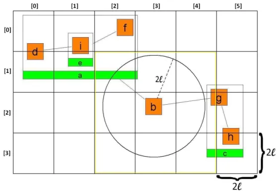
Figure 3.1: A gridded CoSE Graph. The circle around node b indicates the repulsion circle of b.

In order to fill the grid squares, the node list is traversed. Grid coordinates of each node are calculated, and each node is put to its corresponding grid cell(s) by simply adding the node in question to the corresponding collection(s). To easily access the grid cells occupied by a node, start and finish grid coordinates on both x and y axes are maintained for each node. In the sample graph in Figure 3.1, for compound node c, start and finish coordinates on x axis are 4 and 5, and start and finish coordinates on y axis are 1 and 3, respectively. For node b, both start and finish coordinates on x axis is 3.

Nodes that reside in the circular area of the radius 2l around each node are found and stored in a list named surrounding. For obtaining the surrounding list, all occupied cells with their neighbor cells are traversed. Since start and finish coordinates of each node are stored, CoSE will not need to traverse the whole

grid matrix for finding the occupied cells by a node. For instance, for calculating the surrounding of node b in Figure 3.1, all nodes in the highlighted matrix (cells 2 to 4 in x axis and 1 to 3 in y axis) are checked. The nodes in the repulsion circle of b (which is only a for the sample graph) are put to the surrounding list of b. Repulsion circle of b is the circle with a radius of 2l and b is in the center.

In order to achieve the most accurate spring embedder simulation, CoSE needs to update the grid cells before calculating the repulsive forces in each iteration. However, since we are looking for an improvement at the performance, and simu-lating a mechanical system just roughly, updating grid cells periodically is a good solution. Currently, CoSE re-calculates the grid cells for each node once in every ten iteration.

Once surrounding lists of all nodes are constructed, these lists are traversed for each node, and repulsive forces between a node and its surrounding can be calculated cumulatively as in the CoSE.

For nodes v and u, where the distance between them is less than the repulsion range, v is added to the surrounding list of u, only if u is not included in the surrounding list of v. This condition is checked in order not to calculate the repulsive force between a node pair twice. This violates the term of surrounding list, but saves great time in application.

method CalcRepulsionForcesWithFRGridVariant(VertexSet V) 1) if number of iterations is multiple of 10 then

2) construct empty grid cells 3) for all nodes vi ∈ V do

4) calculate start and finish coordinates of vi

5) put vi to corresponding grid cell(s)

6) for all nodes vi ∈ V do

7) for all nodes ui inside the neighbor grid cells of vi do

8) if distance between vi and ui is less than 2l

9) and owner graph of vi and ui are same then

10) add ui to surrounding list of vi

11)for all nodes vi ∈ V do

12) calculate the repulsion forces between vi and its surrounding

Figure 3.2: Repulsive force calculations after the adaptation of FR-Grid Variant method.

3.2

Complexity Analysis

Variable sized nodes not only make it hard for the performance to scale but also the complexity analysis difficult for adapted FR-grid variant method. For convenience, analysis will be done for only fixed-sized nodes with default values 40 × 40 pixels for level = 0 and l = 50 (which is the default value for ideal edge length in CoSE).

Repulsion range r equals 100 with the default values above, which means a node with a 40 × 40 size, can occupy 4 grid cells in the worst case. Thus, number of grid cells to be checked for such a node is 16. As it is described in section 2.4, the number of grid cells is found as |V |₄ , if nodes are evenly distributed, such that one grid cell contains about 4 nodes. In conclusion, approximately 64 nodes are considered for repulsion force calculation of a node, on average, so that complexity of the repulsion force calculation is O(|V |) with a large constant.

Grid cells are refreshed in every ten iteration. This operation has two phases: constructing the grid, and calculating the surroundings of all nodes. Deciding the size of the grid takes constant time. Traversing the node list and putting the nodes in the correct grid cells take O(|V |) time. Thus, total time to construct the grid is O(|V |). In order to calculate the surrounding of each node, neighbor cells are traversed. As we make the analysis for fixed-sized nodes and assume that nodes are distributed uniformly, there will be 16 grid cells to traverse and approximately 64 nodes to add as neighbors. Therefore, total time to calculate surrounding of all nodes is also O(|V |). In conclusion, preparations for FR-grid variant calculation in one iteration costs O(|V |) but since the grid cells are refreshed in every ten iteration, the cost is reasonable on the average.

As a result, the complexity of repulsive force calculation is asymptotically decreased from O(|V2|) to O(|V |).

3.3

Results

Mesh-like, tree-like and compound graphs are generated randomly for testing the execution time of CoSE after adapting the FR-grid variant. Generated meshes are neither dense nor sparse with edge-vertex ratio (|E|_{|V |}) approximately 1.80. For generated trees, probability of a node having children is 0.5, a node can have 1 to 4 children and edge-vertex ratio approximately equals to 1. For generated compound graphs, inter-graph edges are a quarter of all the edges. Number of siblings in a compound node is 4, and compound depth is 2 with a pruning probability of 0.4 for the inclusion tree. Edge-vertex ratio of compound graphs is approximately 0.5. Tests are run on an ordinary PC with Intel(R) Core(TM)2 Quad CPU Q8400 2.67 GHz processor, 3.25 GB usable RAM, and Windows 7 Professional 32-bit operating system. Comparisons of execution times before and after integrating the FR-grid variant to our compound spring embedder are shown in Figure 3.3, Figure 3.4 and Figure 3.5.

Figure 3.3: Execution time comparison with mesh-like graphs (Using FR-grid variant method).

Figure 3.4: Execution time comparison with tree-like graphs (Using FR-grid vari-ant method).

Figure 3.5: Execution time comparison with compound graphs (Using FR-grid variant method).

times after applying the FR-grid variant method. As the size of the input graph increases, difference between the running times increases greatly in line with our theoretical analysis.

3.3.1

Implementation Issues

Currently, CoSE updates the grid cells once in every ten iteration. In the early iterations, the spring embedder is not stable since temperature is high. Because of that, nodes are more likely to make dramatic movements and oscillations, so at the beginning of the spring embedder iterations, occupied grid cells by a node are more likely to change. Moreover, as the system is closer to convergence state, nodes move slightly and less likely to change occupied cells. Thus, in order to obtain more realistic simulations without a huge time penalty, updating grid cells frequently in early stages and increasing the re-calculation period proportional to the number of total iterations passed can be useful.

Chapter 4

Improving by Multi-level Scaling

Strategy

Most of the spring embedder algorithms remain insufficient in laying out large graphs that are especially symmetric or contain a particular structure or a pat-tern. There are several multi-level methods aiming to resolve this problem by recursively coarsening the input graph. When the coarsest graph is constructed, layout process is started. Final positions of the nodes in each laid out coarser graph are interpolated to the finer graph.

We have surveyed through several methods and researched two methods in detail earlier in section 2.5. Because we need a fast, easy, and efficient method, we decided to implement the Walshaw’s clustering method for adapting the multi-level scaling strategy to the CoSE algorithm.

4.1

Adaptation

The most challenging problem of adapting a multi-level scaling method to CoSE is handling compound nodes during the coarsening process. If compound nodes of graph Gi are treated as leaf nodes while Gi is being coarsened, it means all

child nodes of each compound node will be ignored, and only the first hierarchic level of the input graph will be considered during the coarsening. For instance, if the input graph G0 has thousands nodes, but in the root graph, there are

only a few compound nodes that own all other nodes, then G0 would have a

few coarsening levels. Thus, CoSE could not benefit from the advantages of the multi-level scaling method.

We investigated the approach of handling compound nodes during the coars-ening process by coarscoars-ening each level of input graph separately. This would give fine layouts inside each compound node, but would create another problem. Separate hierarchical levels should be put together in order to obtain the final layout. In hierarchical level l, if a child graph exceeds the boundary of its parent node v or shrinks too much, then v should be resized. So the layout of level l − 1 should be computed before level l. This results in a contradictory situation to the inter-graph edges supported by CoSE. The reason is simply that we want to put neighbors close to each other, and so CoSE needs to calculate the attractive forces between nodes connected with an edge but reside on different levels. Due to the reasons mentioned, we had to give up this idea and decided to consider only non-compound nodes during the coarsening process.

A special graph structure named coarsening graph is introduced in order to ease and modularize the coarsening process. In the coarsening graph, only leaf nodes and the intra-graph edges that are between these nodes are included.

4.1.1

Coarsening Algorithm

There is a one-to-one mapping between coarsening graphs and compound graphs. We use Ml notation for the compound graph in coarsening level l, and Gl for the

coarsening graph which contains only the leaf nodes of Ml and the intra-graph

edges between these nodes. Thus, a compound graph Ml indicates the original

graph will be laid out in level l, whereas the coarsening graph Gl is used for only

coarsening purpose. We defined reference pointers in order to maintain the one-to-one mapping from nodes in the coarsening graph to the nodes in the compound

graph.

For coarsening level zero (l = 0), G0 is constructed with no nodes or edges

initially. By a recursive traversal, leaf nodes of M0 are gathered, and for each leaf

node, a corresponding coarsening node is created, and added to G0. In order to

obtain a one-to-one mapping between M0 and G0, leaf nodes of M0 are mapped

with all nodes in G0. After creating and mapping all the nodes in G0, edge list

of M0 is traversed. Only the edges that connects the leaf nodes (excluding the

inter-graph edges) are added to G0. Weight s of all nodes are set to one. By this

way, construction of G0 is completed.

G0 is coarsened recursively, until the size of Gl becomes 1, or size of last two

coarsening graphs Gl and Gl−1 are equal to each other. If |VGl| = |VGl−1|, it

means all nodes in both Gl and Gl−1 are isolated, and no coarser graphs can be

generated any more.

For a coarsening level l, all nodes in Gl are flagged as unmatched. Nodes

of a coarsening graph are stored in a list instead of a set, in order to assure a deterministic search for unmatched nodes. If there is a node in Gl, then the first

node v in the node list is checked, whether it is matched or not. If v is unmatched, then v and if exists, its matching node u are contracted and merged into node t. Unmatched neighbors of v in the same graph are traversed, and the node with the minimum weight is selected for matching. Weight of t is set to the sum of weights of v and u, and t is flagged as matched. Neighbors of v and u are connected to t. Finally, t is added to the end of the node list of Gl, while v and u are removed

(See the Figure 4.1). Coarsening steps of a compound graph are shown in the Figure 4.2 and the Figure 4.3.

Two pointers; previous and next, are used for tracing the coarsening processes and interpolating the final positions of finer graphs to the coarser ones. Each node has two previous pointers, and one next pointer. For instance, let us assume that t ∈ Ml. Nodes v, u ∈ Ml−1, which are merged and contracted to the node t are

pointed by previous pointers of t (see the 4th _{and 6}th _{screenshots in Figure 4.1).}

Figure 4.1: A sample contraction process. a) The initial phase of the coarsening graph, b) v and u are chosen to be matched, c) Node t is created and neighbors of v is connected to the t, d) v is removed from the coarsening graph e) Neighbors of u is connected to the t, f) u is removed from the coarsening graph.

Figure 4.2: Coarsening steps of a compound node. a) The input graph M0, b) g

and h are matched, a new node m ∈ M1 is created, neighbors of g are connected

to m, c) g is removed, d) Neighbors of h are connected to m, e) h is removed, f) d and e are matched, a new node n ∈ M1 is created, neighbors of d are connected

to n, g) d is removed, h) Neighbors of e are connected to n, i) e is removed, j) k and l are matched, a new node o ∈ M1 is created.

Figure 4.3: Coarsening steps of a compound node (Continues from the Figure 4.2). k) Neighbors of k are connected to o, l) k is removed, m) l is removed, n) M1, o) f

and m are matched, a new node p ∈ M2 is created, neighbors of m are connected

method coarsen(CoarseningGraph G=(V,E)) 1) for i ≤ V.size do

2) V [i].matched := false

3) while V [0] is not matched do 4) CoarseningNode v := V [0]

5) CoarseningNode u := lowest weighted neighbor of v 6) _{contract(G, v, u)}

7) for i ≤ V.size do

8) CoSENode newNode:= create a new node 9) newNode.previous1 := V [i].node1.reference 10) V [i].node1.reference.next :=newNode 11) if V [i].node2 is not null then

12) newNode.previous2 := V [i].node2.reference 13) V [i].node2.reference.next :=newNode

Figure 4.4: Coarsening method.

method contract(CoarseningGraph G=(V,E), CoarseningNode v, CoarseningNode u)

1) CoarseningNode t := create a new node 2) add t to the end of V

3) t.node1 := v

4) for i ≤ v.neighbors.size do

5) if v.neighbors[i] is not equal to t then 6) CoarseningEdge e := (t, v.neighbors[i] ) 7) add e to E

8) t.weight := v.weight 9) remove v from V 10)if u is not null then 11) t.node2 := u

12) for i ≤ u.neighbors.size do

13) if u.neighbors[i] is not equal to t then 14) CoarseningEdge f := (t, u.neighbors[i]) 15) add f to E

16) t.weight := t.weight +u.weight 17) remove u from V

18)t.matched := true

After constructing Gl+1 from Gl, coarser compound graph Ml+1 will be

gener-ated from Gl+1. A new root for Ml+1 is created. Then, nodes of Ml are traversed

recursively (where the initial call is made with the root graphs of Ml and Ml+1)

as follows: If current node v is a compound one, then a new compound node y is created with an empty child graph and added to the graph which is passed as parameter. Next pointer of v is set to y and one of the previous pointers of y is set to v. Then, a recursive call is invoked with the child graphs of v and y. If v is not a compound node, then next pointer of v is added to the graph which is passed as parameter. After generating nodes of coarser graph Ml+1, edge list of

Ml is traversed, and edges of Ml+1 are generated.

method generateCoarserCoSEGraph(GraphManager Ml)

1) Create Ml+1

2) Create a root for Ml+1

3) generateNodes( Ml.root, Ml+1.root)

4) generateEdges( Ml.root, Ml+1.root)

Figure 4.6: Generation of coarser CoSE graph from CoarseningGraph. method generateNodes(CoSEGraph Gl = (Vl, El),

CoSEGraph Gl+1 = (Vl+1, El+1))

1) for all nodes of Gl do

2) if a node (vl) is compound then

3) create vl+1 with an empty child graph

4) vl.next := vl+1

5) vl+1.previous1 := vl

6) generateNodes( vl.child vl+1.child)

7) otherwise

8) add vl.next to Gl+1

9) copy geometry of vl to vl+1

Figure 4.7: Generation of nodes of coarser graph. method generateEdges(CoSEGraph Gl= (Vl, El),

CoSEGraph Gl+1 = (Vl+1, El+1))

1) for all edges of Gl do

2) create el with no source or target

3) el.source:= el.source.next

4) el.target := el.target.next

All graphs from the finest to the coarsest are held in a list. Layout phase begins with the coarsest graph Mk−1, where k is the number of levels. Mk−1

is laid out with our compound spring embedder. When layout calculations are finished, final positions of nodes in Mk−1 are used for initial positioning of Mk−2.

As aforementioned, nodes, that are contracted in order to generate a node in a coarser graph, can be accessed via previous pointers. Assume that v ∈ Mk−1 and

previous pointers of v points to the node u and w, where u, w ∈ Mk−2. When

interpolating the positions, node u, which is pointed by the first previous pointer is placed to the exactly same place with v. Node w, the second previous pointer, is placed to the lower right of the first node, to a distance of ideal edge length from both x and y axes. Refinement continues until the input graph M0 is reached.

Whole layout calculation is finished when M0 is laid out.

In the Figure 4.9 and Figure 4.10, laid out levels of a randomly generated mesh-like graph and a compound graph with a particular structure are shown. It is observable that, each coarser graph is an abstraction of the finer one.

4.2

Complexity Analysis

Making the complexity analysis of a multi-level scaling method is not easy, since the number of abstraction levels heavily depends on the structure of the input graph. For dense graphs like complete meshes, it is more probable to find a matching for a node. For the best case, each node is matched with another one which makes number of abstraction level k = log₂|V |. On the other hand, for sparse graphs like trees, more than half of the clusters may contain only one node. For the worst case, only one node is matched with another one, but other nodes match with themselves so that number of abstraction level k = |V | − 1.

Let Tsingle(|V |, |E|) be the running time of a single level force-directed

place-ment algorithm and Tmulti(|V |, |E|) be the running time of the same

algo-rithm after applying Walshaw’s clustering method [11], [9]. Tmulti(|V |, |E|) = k−1

X

i=0

Figure 4.9: A random mesh-like graph M , coarsened in 11 steps. Levels are laid out via CoSE [8] after adapting the Walshaw’s clustering method [11]. On the left-top, there is M10, the coarsest graph, with 2 nodes. On the right-bottom,

Figure 4.10: A compound graph N , with 10 levels. Levels are laid out via CoSE [8] after adapting the Walshaw’s clustering method [11]. On the left-top, there is N9, the coarsest graph, with 3 nodes in the root graph, and 7 nodes in total. On

Tref ine(|Vi|, |Ei|) is the time to refine graph Gi from Gi−1, Tinit(|Vi|, |Ei|) is the

time to make initial placement of Gi and Tcoarsen(|Vi|, |Ei|) is the time to coarsen

graph Gi to Gi+1.

For the best case, Tref ine(|Vi|, |Ei|) and Tcoarsen(|Vi|, |Ei|) are (|Vi| + |Ei|)/2,

because the traversal of half of the node list is enough to refine or coarsen the graph Gi. For the worst case, Tref ine(|Vi|, |Ei|) and Tcoarsen(|Vi|, |Ei|) are

|Vi| − 1, because whole list has to be traversed to refine or coarsen the graph

Gi. Tinit(|Vi|, |Ei|) is |Vi| for any case. In conclusion k−1

X

i=0

(Tref ine(|Vi|, |Ei|) +

Tinit(|Vi|, |Ei|) + Tcoarsen(|Vi|, |Ei|)) is asymptotically linear in |V | and |E|.

For the best case, each cluster contains two nodes, so |Vi+1| = |Vi|/2. Also

for graphs where edge node ratio |E|/|V | is greater than 1, |Ei+1| ≤ |Ei|/2 since

number of nodes in coarser graph is decreased by the factor of 1/2. On the other hand, for the worst case, all clusters but one contain one node, so |Vi+1| = |Vi| − 1

and |Ei+1| ≤ |Ei| − 1. Therefore, k−1 X i=0 Tsingle( |V | 2i , |E| 2i ) ≤ k−1 X i=0 Tmulti(|Vi|, |Ei|) ≤ k−1 X i=0

Tsingle(|V | − i, |E| − i). Lower bound of the inequality is less than 2 ×

Tsingle(|V |, |E|) and upper bound is less than k × Tsingle(|V |, |E|). In

conclu-sion, the inequality above becomes 2 × Tsingle(|V |, |E|) ≤ k−1

X

i=0

Tmulti(|Vi|, |Ei|) ≤

|V | × Tsingle(|V |, |E|).

As a result, as the density increases or the structure of the graph gets closer to the best case, complexity of the multi-level scaling methods is closer to the lower bound, which is asymptotically the same as the single-level methods. However, as the density decreases or the structure of the graph becomes closer to the worst case, complexity converges to the upper bound, which multiplies the complexity of the single-level methods by |V | in theory. But in practice, layout in each level except the first one is incremental, so the system should converge a lot faster than in theory.

4.3

Results

In order to test the execution time and resulting layouts produced by CoSE with Walshaw’s multi-level strategy, mesh-like, tree-like, and compound graphs are generated randomly. For performance comparisons, tests are run with the same graphs and the same system/machine configuration that are used for testing the FR-grid variant. In addition, graphs with a specific structure are manually created for testing the visual quality. Comparisons of execution times before and after adapting the multi-level scaling strategy to our compound spring embedder are shown in Figure 4.11, Figure 4.12 and Figure 4.13.

Figure 4.11: Execution time comparison with mesh-like graphs (Using multi-level scaling strategy).

Walshaw’s clustering method gives better results for mesh-like graphs. On the other hand, it is out-performed by our original spring embedder for tree-like and especially compound graphs. Since the edge-vertex ratio of the tested compound nodes is less than 1, and for trees it is highly probable that more than half of the clusters have only one node, we obtained a worse performance for trees and compound graphs. However, meshes are denser and structured more similar to

Figure 4.12: Execution time comparison with tree-like graphs (Using multi-level scaling strategy).

Figure 4.13: Execution time comparison with compound graphs (Using multi-level scaling strategy).