Risk estimation by maximizing area under receiver operating characteristics curve with application to cardiovascular surgery

RISK ESTIMATION BY MAXIMIZING

AREA UNDER RECEIVER OPERATING

CHARACTERISTICS CURVE WITH

APPLICATION TO CARDIOVASCULAR

SURGERY

A THESIS

SUBMITTED TO THE DEPARTMENT OF COMPUTER ENGINEERING AND THE INSTITUTE OF ENGINEERING AND SCIENCE

OF BĐLKENT UNIVERSITY

IN PARTIAL FULLFILMENT OF THE REQUIREMENTS FOR THE DEGREE OF

MASTER OF SCIENCE

By

Murat Kurtcephe

July 2010

i

I certify that I have read this thesis and that in my opinion it is fully adequate, in scope and in quality, as a thesis for the degree of Master of Science.

Prof. Dr. H. Altay Güvenir (Supervisor)

I certify that I have read this thesis and that in my opinion it is fully adequate, in scope and in quality, as a thesis for the degree of Master of Science.

Assoc. Prof. Dr. A. Rüçhan Akar

I certify that I have read this thesis and that in my opinion it is fully adequate, in scope and in quality, as a thesis for the degree of Master of Science.

Asst. Prof. Dr. Çiğdem Gündüz Demir

Approved for the Institute of Engineering and Sciences:

Prof. Dr. Levent Onural

ii

ABSTRACT

RISK ESTIMATION BY MAXIMIZING AREA UNDER

RECEIVER OPERATING CHARACTERISTICS CURVE

WITH APPLICATION TO CARDIOVASCULAR

SURGERY

Murat Kurtcephe M.S. in Computer Engineering Supervisor: Prof. Dr. H. Altay Güvenir

June 2010

Risks exist in many different domains; medical diagnoses, financial markets, fraud detection and insurance policies are some examples. Various risk measures and risk estimation systems have hitherto been proposed and this thesis suggests a new risk estimation method. Risk estimation by maximizing the area under a Receiver Operating Characteristics (ROC) curve (REMARC) defines risk estimation as a ranking problem. Since the area under ROC curve (AUC) is related to measuring the quality of ranking, REMARC aims to maximize the AUC value on a single feature basis to obtain the best ranking possible on each feature. For a given categorical feature, we prove a sufficient condition that any function must satisfy to achieve the maximum AUC. Continuous features are also discretized by a method that uses AUC as a metric. Then, a heuristic is used to extend this maximization to all features of a dataset. REMARC can handle missing data, binary classes and continuous and nominal feature values. The REMARC method does not only estimate a single risk value, but also analyzes each feature and provides valuable information to domain experts for decision making. The performance of REMARC is evaluated with many datasets in the UCI repository by using different state-of-the-art algorithms such as Support Vector Machines, naïve Bayes, decision trees and

iii

boosting methods. Evaluations of the AUC metric show REMARC achieves predictive performance significantly better compared with other machine learning classification methods and is also faster than most of them.

In order to develop new risk estimation framework by using the REMARC method cardiovascular surgery domain is selected. The TurkoSCORE project is used to collect data for training phase of the REMARC algorithm. The predictive performance of REMARC is compared with one of the most popular cardiovascular surgical risk evaluation method, called EuroSCORE. EuroSCORE is evaluated on Turkish patients and it is shown that EuroSCORE model is insufficient for Turkish population. Then, the predictive performances of EuroSCORE and TurkoSCORE that uses REMARC for prediction are compared. Empirical evaluations show that REMARC achieves better prediction than EuroSCORE on Turkish patient population.

Keywords: Risk Estimation, AUC Maximization, AUC, Ranking, Cardiovascular Operation Risk Evaluation

iv

ÖZET

RECEIVER OPERATING CHARACTERTICS EĞRĐSĐ

ALTINDAKĐ ALANI MAKSĐMĐZE EDEREK RĐSK

TAHMĐNĐ VE KARDĐYOVASKÜLER CERRAHĐ

UYGULAMASI

Murat Kurtcephe

Bilgisayar Mühendisliği Bölümü Yüksek Lisans Tez Yöneticisi: Prof. Dr. H. Altay Güvenir

Temmuz 2010

Risk birçok farklı alanda mevcuttur; tıbbi tanı, finansal piyasalar, dolandırıcılık tespiti ve sigorta poliçeleri bunların birkaçıdır. Çeşitli risk ölçütleri ve risk tahmin sistemleri bugüne kadar önerildi ve bu tez yeni bir risk tahmini yöntemi sunmaktadır. Receiver Operating Characteristics (ROC) eğrisi altındaki alanı maksimize ederek risk tahmin yöntemi (REMARC), risk tahmini bir sıralama sorunu olarak tanımlar. ROC eğrisi altındaki alan (AUC) değeri sıralama kalitesini ölçme ile ilgili olduğundan, REMARC tek bir öznitelik üzerinde en yüksek AUC’yi elde ederek her öznitelik üzerinde mümkün olabilecek en iyi sıralamayı sağlamayı hedeflemetedir. Verilen bir kategorik öznitelik için, herhangi bir risk yordamının en yüksek AUC’yi elde etmek için sağlaması gereken şartın ne olduğunu ispatladık. Sayısal öznitelikler de ölçüt olarak AUC’yi kullanan bir yöntemle ayrıklaştırılmıştır. Sonra, sezgisel bir yaklaşımla AUC’nin maksimize eldilmesi tüm veriseti üzerine genişletilmiştir. REMARC eksik verileri, ikili sınıfları, sürekli ve kategorik öznitelikleri işleyebilir. REMARC yöntemi sadece risk değeri tahmin etmekle kalmaz aynı zamanda her bir öznitelik üzerinde analiz yapar ve karar verme esnasında alan uzmanlarına değerli bilgiler sağlar. REMARC’ın performansı, UCI veriseti deposundan elde edilen birçok veri seti ile support vector machine naïve Bayes, decision trees (karar ağaçları) ve boosting (arttırma) yöntemleri gibi modern

v

algoritmalar kullanılarak değerlendirilmiştir. AUC ölçütüyle yapılan değerlendirmeler göstermektedir ki REMARC diğer birçok makina öğrenmesi yönteminden önemli derecede daha iyi tahmin performansına sahiptir ve diğer yöntemden çoğundan daha hızlı çalışmaktadır.

Kardiyovasküler cerrahi alanı, REMARC yöntemi ile yeni risk tahmini çerçevesi oluşturmak amacıyla seçilmiştir. TurkoSCORE projesi, REMARC algoritmasının öğrenme aşaması için veri toplamak amacıyla kullanıldı. REMARC’ın tahmin performansı, en popüler kardiyovasküler cerrahi riski değerlendirme yöntemlerinden biri olan EuroSCORE ile karşılaştırıldı. EuroSCORE Türk hastalar üzerinde değerlendirildi ve EuroSCORE modelinin Türk nüfusü için yeterli olmadığı gösterildi. Sonra, EuroSCORE ve tahmin için REMARC kullanan TurkoSCORE’un tahmin performansı karşılaştırldı. Deneysel değerlendirmeler göstermektedir ki REMARC Türk hasta popülasyonunda EuroSCORE’a göre daha iyi tahmin performansı göstermektedir.

Anahtar Kelimeler: Risk Tahmini, AUC azamileştirme, AUC, Sıralama,

vi

Acknowledgements

This thesis would not have been possible without the great support I have received from some special people. First of all, I am heartily thankful to my supervisor Prof. Dr. Halil Altay Güvenir. During these two years I realized that I could not have asked for a better person to guide me in my research. He has been a great mentor from whom I learned a lot. It was a great pleasure to work with him in this thesis.

I grateful to know these incredible people, Serkan Durdu and Çağın Zaim, in the Department of Cardiovascular Surgery at Ankara University who supported me in my research. Specially, I am indebted to Assoc. Prof. Dr. Rüçhan Akar for his invaluable suggestions during my research. Without his dedication, some parts of this thesis could not be completed.

I would like to thank to Asst. Prof. Dr. Çiğdem Gündüz Demir for accepting to read and review this thesis. I would like to show my gratitude to TUBITAK (The Scientific and Technological Research Council of Turkey) since they have supported me in my master studies.

I would like to thank members of room EA511; Can, Volkan, Funda for their valuable friendship. I would specially like to thank to my collage Gönenç for his valuable comments during my researches.

Last but not least, I would like to thank to my parents, Pervin and Yahya for their love and support that always kept me motivated. Without them I would not be able to come so far. Finally, I would like to thank my beloved fiancée Betül

vii

for being in my life and for her undying support. Nothing would be the same without her.

viii

ix

Contents

2.1.3 Risk Estimation in Machine Learning...7

2.2ROC,AUC AND AUC MAXIMIZATION...8

2.2.1 Receiver Operating Characteristics (ROC) ...8

2.2.2 Area under the ROC Curve (AUC)... 12

2.2.3 Why AUC is More Proper than Accuracy... 12

2.2.4 AUC Maximization ... 14

2.3DISCRETIZATION... 15

3. REMARC... 17

3.1REMARCINTRODUCTION... 17

3.2SINGLE CATEGORICAL FEATURE CASE... 18

3.2.1 The Effect of the Class Label Choice on a Feature’s AUC ... 24

3.2.2 An Example Toy Dataset... 25

3.3HANDLING CONTINUOUS FEATURES... 26

3.3.1 The MAD Method ... 27

3.3.2 A Toy Dataset Discretization Example ... 29

3.4REMARCALGORITHM... 30

3.5INTERPRETATION OF THE REMARCPREDICTIVE MODEL... 32

3.6EMPIRICAL EVALUATIONS... 33

3.6.1 Predictive performance... 34

3.6.2 Running Time ... 36

4. TURKOSCORE: TURKISH SYSTEM FOR CARDIAC OPERATIVE RISK EVALUATION ... 39

x

4.2EUROSCORE ... 40

4.3EUROSCOREVALIDATION ON TURKISH PATIENTS... 42

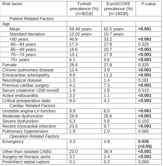
4.3.1 Demographic results... 42

4.3.2 Model Calibration and Discrimination... 44

4.4COMPARISON OF REMARC AND EUROSCORE ... 46

4.5REMARCBASED CARDIOVASCULAR RISK ESTIMATION SYSTEM... 48

5. CONCLUSION AND FUTURE WORK ... 53

A EUROSCORE ... 65

xi

List of Figures

2.1 ROC curves of the REMARC method with TurkoSCORE risk factors... 9

2.2 ROC graph of the given toy dataset in Table 1 including the y=x line in order to show random performance... 11

3.1 Effect of swapping the risk values of two feature values ... 20

3.2 Relation between the slopes of two consecutive line segments in a convex ROC curve... 21

3.3 Visualization of the ROC points in a two-class discretization... 29

3.4 Final cut-points after the first pass of convex hull algorithm ... 30

3.5 Algorithm of the REMARC method’s training phase. ... 31

3.6 Testing phase algorithm of the REMARC method ... 32

4.1 ROC curves for both Logistic and Standard EuroSCORE for whole cohort ... 45

4.2 ROC curves for both Logistic and Standard EuroSCORE for isolated CAGB cohort ... 46

4.3 ROC curves for both Logistic EuroSCORE, Standard EuroSCORE and REMARC with EuroSCORE risk factors... 47

xii

List of Tables

2.1 A Toy dataset given with hypothetical scores... 11

3.1 Toy training dataset with one categorical feature ... 26

3.2 Training datasets risk values are calculated and instances are sorted in

ascending order ... 26

3.3 Negated version of the training dataset. The risk values are calculated again

and instances are sorted in ascending order... 26

3.4 A toy dataset for visualizing MAD in two-class problems. The name of the

attribute to be discretized is F1 ... 29

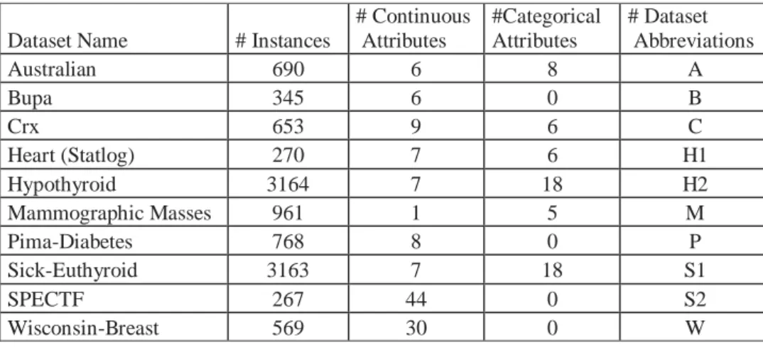
3.5 Properties of the datasets used in the empirical evaluations of the

REMARC algorithm... 34

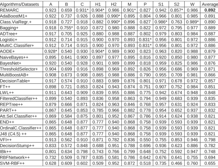
3.6 The comparison of the predictive performance of REMARC algorithm with

other algorithms on AUC metric. 10 datasets are used during evaluation.

Algorithms marked with ++ are outperformed by REMARC method with a

statistically significant difference Algorithms marked with + are

outperformed by REMARC on average with no significant difference.

AUC values marked with * are the best AUC values for that dataset

xiii

3.7 The comparison of the average running time performance of REMARC

algorithm with other algorithms (in ms) . 10 datasets are used during

evaluation. Algorithms marked with ++ symbol are outperformed by

REMARC method on running time basis with a statistically significant

difference. Algorithms marked with -- symbol outperformed REMARC

method on running time basis with a statistically significant difference. +

marked algorithms are outperformed by REMARC on average and –

marked algorithms outperform REMARC on average with no significant

difference. AUC values marked with * are the best AUC values for that

dataset (Lower results better) ... 37

4.1 Prevelances of risk factors in Turkish and EuroSCORE population. The

risk factors that have significant difference are shown in bold face.

EuroSCORE prevelance values are taken from Roques et al. [84] ... 43

4.2 Predicted and observed mortality by EuroSCORE risk level for whole

cohort. In logistic EuroSCORE analysis, patients are divided into three

approximately equal risk quintiles ... 44

4.3 Predicted and observed mortality by EuroSCORE risk level for isolated

CABG cohort. In logistic EuroSCORE analysis, patients are divided into

three approximately equal risk quintiles ... 45

4.4 26 Different datasets are formed by eliminating the instances with missing

values. Dataseti contains at most i many missing features from 28 features

Number of instances, p, n values and AUC values are given. AUC values of

xiv

A.1 TurkoSCORE approximations ... 66

B.1 AUC values of EuroSCORE risk factors ... 67

B.2 TurkoSCORE selected features and AUC values of each feature. AUC

values are calculated by using ten-fold cross validation ... 68

B.3 TurkoSCORE selected features and AUC values of each feature. AUC

values are calculated by using whole dataset as training set ... 69

1

Chapter 1

Introduction

Accurate prediction of risk is essential for life. Avoiding or being aware of risks in domains such as finance or medicine can save money and lives, respectively. The main motivation behind the research on risk-prediction systems is to improve system performance to avoid unwanted events or negative consequences.

This thesis proposes a new risk measure and a supervised machine learning algorithm to estimate the values of this measure. The algorithm, learning from training instances, develops a mode of the domain based on receiver operating characteristics (ROC) analysis, so that the area under ROC curves (AUC) of ordering the instances will be maximized [1]; hence, the algorithm is called Risk Estimation by Maximizing the Area under ROC Curve (REMARC).

Specific risk estimation methods have been developed for finance [2] medicine [3, 4] and insurance [5] to name some examples. Some methods are dependent on statistical models while some are based on machine learning algorithms. The machine learning algorithms are usually classification

2

algorithms that can associate a certainty factor with their classification. The certainty factor for a predicted unwanted case is taken as the value of risk.

The word “risk” is generally taken to mean “an unwanted situation” [6]. Although these unwanted cases may be severe, their likelihood of occurrence is usually rare. Therefore, datasets for such domains usually are unbalanced and the costs of misclassification are not symmetric. Classification algorithms that aim to maximize accuracy are not suitable for such unbalanced datasets [7, 8, 9]. Instead, an alternative metric called AUC, proposed by Bradley, is the evaluation metric to maximize [10]. AUC has important features such as insensitivity to class distribution and cost distributions [10, 11, 9], which make it suitable for risk domains.

In risk domains, representing the risk score as a real value between 0 and 1 may not be sufficient, and even misleading; relatively ordering instances in terms of risk values may be much more informative. For example, instances can be located on a single dimension, where the safest cases are on one side and the riskiest cases are on the other side. Since it has been shown by Hanley and McNeil that AUC is able to qualify ranking instances, maximizing AUC also leads to the best ranking [1]. Recent research on maximizing AUC by Toh et al. [12] and Rakotomamonjy also shows the importance of ranking instances [13].

The REMARC method is not able to handle continuous data without preprocessing. All continuous features should be discretized first. In this thesis in addition to the REMARC method, a discretization method called Maximum Area under ROC curve based Discretization (MAD) is proposed.

The main contributions of the REMARC algorithm can be shown in three different ways. First, we show the conditions a risk scoring function must possess in order to achieve maximum AUC for a single feature dataset case. Second, the maximization of AUC is extended over the whole dataset by using a

3

simple heuristic, which also depends on AUC’s metric. Lastly, the human readable model formed by REMARC helps domain experts by indicating what features and how their particular values affect the risks.

Cardiovascular surgery domain is selected as a test domain for REMARC. There are important reasons behind this choice. First of all, risk evaluation methods are being used in order to inform cardiac patients properly about the mortality risk of surgery by taking into consideration risk factor of patients. The predictions obtained by using these methods are also valuable for monitoring the surgical care and checking the surgical quality with the accepted norms. Since the patients risk factors are taken into consideration, operative mortality can be used as a measure of surgical quality. Therefore, different machine learning approaches have been proposed to predict mortality risks of patients undergoing cardiovascular surgeries [14, 15, 16, 17].

EuroSCORE risk model is learned by using nearly 20 thousand patients from 128 hospitals in eight European countries [14]. EuroSCORE method has been used in Turkish cardiovascular surgery departments in order to assess mortality risk of patients. Validation of EuroSCORE has been analyzed in countries outside of Europe [18, 19]. According to these researches, there exist crucial differences between the patient populations across the nations. As a result, the EuroSCORE risk prediction model is not validated in some patient populations. Therefore, in this thesis the evaluation of EuroSCORE model on Turkish patients is analyzed. After analyzing EuroSCORE model on Turkish population, the predictive performance of REMARC used in TurkoSCORE system is compared with EuroSCORE. Since REMARC performs better than EuroSCORE, the REMARC algorithm is proposed as a new cardiovascular surgery risk estimation system.

In the next chapter, literature summary about the risks, risk domains, ROC, AUC, AUC maximization, discretization are given. Chapter 3 covers the

4

theoretical background of the REMARC method, implementation details and empirical evaluation of REMARC. In Chapter 4, REMARC is applied to cardiovascular surgery domain and compared by EuroSCORE model. Finally, Chapter 5 concludes with some directions for future work.

5

Chapter 2

Background

In this chapter, the background information needed to understand the concepts in the following chapters is provided. The risk subject is investigated in detail. The ROC and AUC subjects are given since they are essential in REMARC. AUC maximization subject is discussed in this chapter, as well. Discretization subject is also investigated in order to provide background information for the MAD method.

2.1 Risks

Risk has always been a normal occurrence. Risks such as a complication from surgery, a fraudulent financial transaction, a firm going into financial distress and an e-mail being spam are all part of today’s world. Giddens claims that the ideas of risk and responsibility are closely linked in a risk society, and suggests that legal theorists and practitioners should also concern themselves with the idea and reality of risk [6]. The word “risk” is commonly used in daily life, because of its popularity in the media, however, a formal definition is needed.

6

2.1.1 Definitions of Risk

Hansson gives five definitions of risk commonly used in different disciplines [20]. Hansson’s third definition is the most suitable for defining the risk used in this thesis: “The probability that an unwanted event may or may not occur”. For example, the risk of a credit card transaction being fraudulent is 17%.

2.1.2 Risk Domains

Risk implies an unwanted situation. In medicine, mortality and morbidity are two unwanted situations. In finance, money loss and bankruptcy are examples. Since the consequences of these situations are crucial, in order to avoid them extensive research continues on this subject. As an example, it is possible to find books written on specific domains such as process management systems risk estimation [21].

According to Shishkin and Savkov some of the most popular commercial risk analysis tools for financial domains are “Risk Watch” (www.riskwatch.com, USA) and “Commercial Risk Analysis and Management Methodology- CRAMM” (www.cramm.com) [22]. Other than the commercial tools, concepts such as Value-At-Risk (VAR) and other models can be found in literature [2], [23]. Stoyan et al. provide a survey on stochastic models for risk estimations [24]. Recently, Ferrari and Paterlini proposed a new risk estimation method that claims a better performance than VAR [25].

In medicine, a risk scoring system based on logistic regression for cardiovascular surgery is proposed by Roques et al. [26]. Other scoring systems for the same domain also exist [3, 27]. A recent study by D'Agostino et al. shows that some of these scoring systems [4] use Cox regression methods, which is proposed by Cox [28].

7

2.1.3 Risk Estimation in Machine Learning

Risk estimation is not yet a major subarea of machine learning literature. Classification algorithms, which are able to output the confidence or probability of classification results, can be used to approximate risk estimation.

In a risk estimation system, a risk function that assigns higher values to risky instances than safer instances is crucial. In such a system, risk will be computed as a real value between 0 and 1, where 1 indicates the definite risk while 0 represents the safest situation. However, the absolute value of this risk score is also very important for the user. Assume risk() is a function that returns a real number between 0 and 1 as the estimation of the risk. Another risk function,

risk’(), defined as risk(), also returns a value between 0 and 1. Both of these functions will rank the instances in the same order, although their absolute risk values are different.

On any dataset gathered from a risk domain, two classes should be determined in order to distinguish a risky situation from a safe one. In this thesis, we will define these class labels as p (positive, unwanted class) and n

(negative, safe class). For example, in a loan dataset, the class label p indicates a default, while label n indicates that the loan amount has been paid back.

Machine learning techniques have been applied to different domains in order to predict risk. In medicine, Colombet et al. evaluated three different machine learning algorithms in order to predict cardiovascular surgery risk [29]. Biagioli

et al. used Bayesian models to predict risks in coronary artery surgery

operations [30] and Gamberger et al. evaluated machine learning results on a heart database [31]. Financial domains have also taken advantage of machine learning algorithms. Galindo and Tamayo evaluated machine learning and statistical methods in order to predict credit risks [32]. Kim proposed a financial time series prediction system by using a support vector machine (SVM) [33] and

8

Min and Lee tried to predict bankruptcy risk by using optimal kernel functions for SVM [34]. However, to the best of our knowledge, a risk estimation system that aims to maximize the AUC metric has never been proposed. The ROC curves and AUC metric will be examined in detail before explaining the REMARC method. The next section elaborates on the features of ROC and AUC and their appropriateness for this thesis.

2.2 ROC, AUC and AUC maximization

Since their application to machine learning, ROC graphs and the AUC metric have become popular; AUC is used in evaluating machine learning algorithms and as a learning criterion. We explain the properties that make AUC a better metric than accuracy and discuss the existing research on AUC maximization.

2.2.1 Receiver Operating Characteristics (ROC)

The first application of ROC graphs dates back to World War II, where they were used to analyze radar signals [35]. Since then, they have been used in areas such as signal detection and medicine [36, 37, 38]. The first application to machine learning is done by Spackman [39]. According to Fawcett’s definition, the ROC graph is a tool that can be used to visualize, organize and select classifiers based on their performance [9]. It has become a popular performance measure in the machine learning community after it has been realized that accuracy is often a poor metric to evaluate classifier performance [40, 41, 11].

The ROC literature is more established to deal with binary classification (two classes) problems than multi-class ones. At the end of the classification phase, some classifiers simply map each instance to a class label (discrete output). Some classifiers are able to estimate the probability of an instance belonging to a specific class such as naïve Bayes or neural networks (continuous valued output, also called score). Classifiers produce a discrete output represented by only one point in the ROC space, since only one confusion matrix is produced

9

from their classification output. Continuous-output-producing classifiers can have more than one confusion matrix by applying different thresholds to predict class membership. In this thesis, all instances with a score greater than the threshold are predicted to be p class and all others are predicted to be n class. Therefore, for each threshold value, a separate confusion matrix is obtained. The number of confusion matrices is equal to the number of ROC points on an ROC graph. With the method proposed by Domingos, it is possible to obtain ROC curves even for algorithms that are unable to produce scores [42].

ROC space is two dimensional space with a range of (0.0, 1.1) on both axes. In ROC space the y-axis represents the true positive rate (TPR) of a classification output and the x-axis represents the false positive rate (FPR).

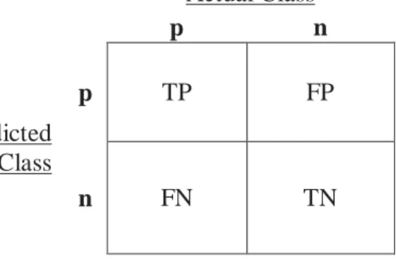
To calculate TPR and FPR values, the definitions of the elements in the confusion matrix must be given. The structure of a confusion matrix is shown in Figure 2.1. True positives (TP) and false positives (FP) are the most important elements of the confusion matrix for ROC graphs. For each threshold value, TP is equal to the number of positive instances (those that have been classified correctly) and FP is equal to the number of negative instances (those that have been misclassified). Actual Class p n p TP FP Predicted Class n FN TN Column Totals: P N

10

TPR and FPR values are calculated by using Eq. 2.1. In this equation N is the

number of total negative instances and P is the number of total positive instances. P TP TPR= / F FP FPR= / Eq. 2.1

As mentioned above, the classifiers producing continuous output can form a curve since they are represented by more than one point in the ROC graph. To draw the ROC graph, different threshold values are selected and different confusion matrices are formed.

By varying the threshold between -∞and +∞, an infinite number of ROC points can be produced for a given classification output. However, this operation is computationally costly and it is possible to form the ROC curve more efficiently with other approaches.

As proposed by Fawcett, in order to calculate the ROC curve efficiently, classification scores are sorted in an increasing order first [9]. Starting from -∞, each distinct score element is taken as a threshold; TPR and FPR values are calculated using Eq. 2.1.

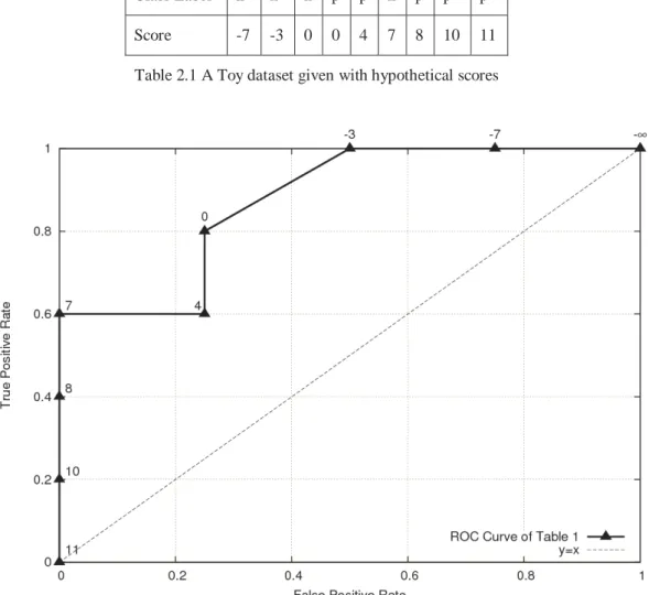
As an example, assume that the score values for test instances and actual class labels for a toy dataset are given in Table 2.1. The ROC curve for this toy dataset is shown in Figure 2.2. In this figure, each ROC point is given with the threshold value used to calculate it. In a dataset with S distinct classifier scores, there are S+1thresholds including -∞ and the same number of ROC points. Since there are eight distinct score values in this toy dataset, there are nine ROC points. With this simple method it is possible to calculate the ROC curve in linear time.

11

Class Label n n n p p n p p p

Score -7 -3 0 0 4 7 8 10 11

Table 2.1 A Toy dataset given with hypothetical scores

Figure 2.2 ROC graph of the given toy dataset in Table 1 including the y=x line in order to show random performance.

It is possible to divide the ROC space into three regions: the region above

y=x line, the area below y=x line and the points on the y=x line. The points on y=x line represent random performance. As an example, a classifier that has a

point on (0.6,0.6) guesses the positive class 60% correctly, however it also has a 60% false positive rate. The points above the y=x line are those belonging to the classifiers that have an acceptable trade-off between the positive and negative classes; similarly, the points below the y=x line correspond to an unacceptable classification performance. A classifier’s ROC point below the diagonal line can be negated by simply inverting the decision criteria of the classifier, replacing all p class labels with n class labels and vice versa. According to Flach and Wu

12

classifiers below the diagonal have valuable information, but they are not able to use it [43].

2.2.2 Area under the ROC Curve (AUC)

ROC graphs are useful to visualize the performance of a classifier but a scalar value to compare classifiers is needed. In the literature, Bradley proposes the area under the ROC curve as a performance measure [10]. According to the AUC measure, the classifier with a higher AUC value performs better in general. A classifier can be outperformed by another classifier in some regions of ROC space, for some specific threshold values, even though the classifier, which has larger AUC, is better than the other.

The ROC graph space is a one-unit square. The highest possible AUC value is 1.0, which represents the perfect classification. In ROC graphs a 0.5 AUC value means random guessing has occurred and values below 0.5 are not realistic as they can be negated by changing the decision criteria of the classifier.

The AUC value of a classifier is equal to the probability that the classifier will rank a randomly chosen positive instance higher than a randomly chosen negative instance. Hanley and McNeil show that this is equal to the Wilcoxon test of ranks [1].

2.2.3 Why AUC is More Proper than Accuracy

There are several reasons why we chose AUC as a learning criterion in this thesis. The first reason is the independence of the decision threshold of the AUC metric. Since the risk estimation methods are not actual classifiers, unless a threshold is fixed it is not possible to calculate an accuracy value. As mentioned in Section 2.1.3, the first task of a risk estimation method is ranking instances correctly. Since AUC has the ability to measure the quality of ranking, it is better than accuracy metric on this basis.

13

Another reason regards the discrimination power of the accuracy and AUC metrics. Bradley was the first author to question the applicability of accuracy metrics in classifier algorithms and to recommend the use of AUC instead [10]. Provost et al. also questioned the applicability of accuracy metrics in classification algorithms and suggested ROC analysis as a powerful alternate tool [41]. Rosset claimed that even if the goal is to maximize accuracy, AUC may be better than empirical error for discriminating between models [44]. The formal proof of the superiority that AUC has over accuracy is later given by Huang and Ling [11]. In their work, the authors showed that AUC is a statistically consistent and more discriminating metric than accuracy. These works clearly show the discriminatory power of the AUC metric.

Skewed (unbalanced) datasets is another reason to prefer AUC as a metric. This situation occurs when the difference between class priors is high. Risk areas such as medicine [45, 8] and fraud detection [46] are examples of skewed datasets. For example, a classifier that predicts all instances as negative even though a few of the instances achieve very high accuracies is misleading [13]. In addition, class distribution can change over time. For example, if in a financial crisis a large number of banks claim bankruptcy, this can change class distribution drastically. In order to solve such problems, AUC, which is insensitive to class distributions, is preferred.

Lastly, misclassification costs cannot be determined for most risk domains. As noted above, skewed datasets are common in real life. In a domain with unbalanced class distribution, when the true misclassification cost is higher than implied by the distribution of training set examples, this situation becomes problematic [47]. Since AUC is also insensitive to misclassification cost, it is preferred in this thesis [48].

14

2.2.4 AUC Maximization

Most classification algorithms are designed to maximize accuracy (or error rate). Since accuracy is a classification performance criterion, algorithms that maximize it give better predictive performance. However, because of the aforementioned drawbacks to the accuracy metric for some domains, AUC has become more popular. It has been shown that maximizing accuracy does not lead to maximizing AUC [49, 50]. As a result, new algorithms maximizing AUC have been proposed.

Some approximation methods to maximize the global AUC value have been proposed by researchers [51, 50, 52]. Ferri et al. proposed a method to locally optimize AUC in decision tree learning [53], and Cortes and Mohri proposed boosted decision stumps [49]. To maximize AUC in rule learning, several new algorithms have been proposed [54, 55, 56]. A nonparametric linear classifier based on the local maximization of AUC was proposed by Marrocco et al. [57]. A ROC-based genetic learning algorithm has been proposed by Sebag et al. [7]. Marrocco et al. used linear combinations of dichotomizers for the same purpose [58]. Freund et al. gave a boosting algorithm combining multiple rankings [59]. Cortes and Mohri showed that this approach also aims to maximize AUC [49]. A method by Tax et al. that weighs features linearly by optimizing AUC has been proposed and applied to the detection of interstitial lung disease [8]. Ataman et al. advocate an AUC-maximizing algorithm with linear programming [60]. Rakotomamonjy suggested rank optimizing kernels for SVMs to maximize AUC [13]. Ling and Zhang compare AUC-based Tree-Augmented Naïve Bayes (TAN) and error-based TAN algorithms; the AUC-based algorithms are shown to produce more accurate rankings [61]. More recently, Calders and Jaroszewicz proposed a polynomial approximation of AUC to optimize it efficiently [62]. Linear combinations of classifiers are used to maximize AUC in biometric scores fusion in Toh et al. [12]. Han and Zhao propose a linear classifier based on active learning, which maximizes AUC [63].

15

2.3 Discretization

Discretization methods aim to find the cut-points that form the intervals in the process of discretization. A continuous attribute is then treated as a discrete attribute whose number of intervals is known on the continuous space.

Liu et al. categorized discretization algorithms on four axes [64]. These categories include supervised vs. unsupervised, splitting vs. merging, global vs.

local, and dynamic vs. static.

Simple methods such as equal-width or equal-frequency binning algorithms do not use class labels for instances during the discretization process [65]. These methods are called unsupervised discretization methods. To improve the quality of the discretization, methods that use class labels are proposed; they are referred to as supervised discretization methods. Splitting methods take the given continuous space and try to divide it into small intervals by finding proper cut-points, whereas merging methods handle each distinct point on the continuous space as an individual candidate for a cut-point and merges them into larger intervals. Some discretization methods process localized parts of the instance space during discretization. As an example, the C4.5 algorithm handles numerical values by using a discretization (binarization) method that is applied to localized parts of the instance space [66, 67]; these methods are called local

methods. Methods that use the whole instance space of the attribute to be

discretized are called global methods. Dynamic discretization methods use the whole attribute space during discretization and perform better on data with interrelations between attributes. Conversely, static discretization methods discretize attributes one by one and assume that there are no interrelations between attributes. According to the categories defined above, MAD is a supervised, merging, global, and static discretization method.

16

Splitting discretization methods usually aim to optimize measures such as entropy [68, 69, 70, 71, 72], which aims to obtain pure intervals, dependency [73] or accuracy [74] of values placed into the bins. On the other hand, the merging algorithms proposed so far use the chi-squarestatistic [75, 76, 77]. As far as we know, the ROC Curve has never been employed in the discretization domain.

17

Chapter 3

REMARC

This chapter presents detailed information about the REMARC method. First of all, a brief introduction to REMARC is given. Then, the risk function designed for categorical features to maximize AUC and the details of the MAD method and its application to REMARC is given. The REMARC method and its implementation are detailed. Finally, in the empirical evaluations REMARC method is compared with other machine learning on real life datasets and results are discussed.

3.1 REMARC Introduction

REMARC is a risk estimation method designed to maximize the AUC metric. The REMARC algorithm reduces the problem of finding a risk function for the whole set of features into finding a risk function for a single categorical feature, and then combines these functions to form one risk function covering all features. We will show here that it is possible to determine risk functions that achieve the maximum AUC for a single categorical feature. REMARC discretizes the numerical features by an algorithm called MAD, proposed by

18

Kurtcephe and Guvenir [78]. The MAD method discretizes a continuous feature in a way that results in a categorical feature by maximizing the AUC.

For a given query, REMARC outputs a real value r in the range of [0,1] as the estimated risk of being the unwanted state. This r value is roughly the probability that the query instance will be in the p class. It is only a rough estimate of probability, since it is very likely that no other instance with exactly the same feature values has been observed in the training set. The REMARC algorithm determines this estimated probability by computing the weighted average of probabilities computed on single features. The weight of a feature is a linear function of its AUC value calculated by the risk estimates for each instance in the training set. A higher value of AUC for a feature is an indication of its higher relevance in determining the class label.

3.2 Single Categorical Feature Case

A categorical feature has a finite set of choices. Let V = {v1, v2, … vn } be a

categorical feature and vi be a categorical value that feature V can take. The

dataset D is a set of instances represented by a vector of n values and class label as <v,c>, where v∈V and c∈ {p,n}

Given a dataset D with a single categorical feature whose value set is V = {v0,

v1,…, vn}, a risk function r: V → [0,1] can be defined to rank the values in V. According to this risk function, a value vi comes after a value vj if and only if

r(vi) > r(vj); hence r defines a partial ordering on the set V. A pair of consecutive values vi and vi+1 defines a ROC point Ri on the ROC space. The coordinates of the point Ri are (FPRi, TPRi).

Theorem 1: Let D be a dataset with a single categorical feature whose value set is V = {v0, v1, …, vn}. Let r: V → [0,1] be the risk function that orders the values of V, as vi+1 comes after vi if r(vi+1) > r(vi), for all values of 0≤i<n. If the values

19

of the risk function for two consecutive values vi and vi+1 are swapped, then the only change in the ROC curve is that the ROC point corresponding to the vi and

vi+1 values moves to a new location so that the slopes of the line segments adjacent to that ROC point are swapped.

Proof: The slope of the line segment between two consecutive ROC points Ri and Ri+1 is 1 1 + + − − = i i i i i FPR FPR TPR TPR s . Since P TP TPR i i = and N FP FPR i i = , 1 1 + + − − = i i i i i FP FP TP TP P N s .

Further replacing TPi =Pi+TPi+1andFPi =Ni+NPi+1, where Pi is the number

of p-labeled instances with value vi, and Ni is the number of n-labeled instances with value vi. i i i N P P N s = .

Similarly, the slope of the line segment connecting the ROC points between Ri+1 and Ri+2 is

1 1 1 + + + = i i i N P P N s .

When the ranking of values vi and vi+1 are changed, only the following changes take place:

, ' , ' , ' , ' 1 1 1 1 + + + + = = = = i i i i i i i i N N N N P P P P j j j j i i j N N P P

j

∀

With this change, only the ROC point Ri at (FPRi, TPRi) is replaced with a new ROC point R’i at (FPR’i, TPR’i). The slopes of the new line segments adjoining R’i are i i i N P P N s ' ' ' = and 1 1 1 ' ' ' + + + = i i i N P P N s .

20

Replacing the new count values with the old ones,

1

'i=si₊

s ands'i+1=si are obtained. ■

For example, consider the dataset given below:

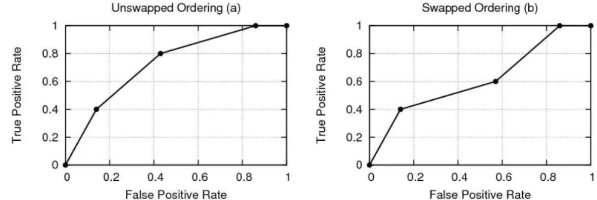
D={(a,n), (b,p), (b,n), (b,n), (b,n), (c,p), (c,p), (c,n), (c,n), (d,p), (d,p), (d,n)}, where V = {a, b, c, d}. If a risk function r orders the values of V as r(a) < r(b) < r(c) < r(d), the ROC curve shown in Figure 3.1a will be obtained. On the other hand, if the rankings of values b and c are swapped, the ROC curve shown in Figure 3.1b will be obtained. A similar technique was used earlier by Flach and Wu to create better prediction models for classifiers [43].

Figure 3.1 Effect of swapping the risk values of two feature values

Theorem 1 shows how concavities in a ROC curve can be removed, resulting in a larger AUC. The next question is how to form the convex ROC curve. The following theorem sets the necessary and sufficient condition for risk functions to satisfy so that their ROC curves are convex.

Theorem 2: Let D be a dataset with a single categorical feature that takes values from the set V = {v0, v1, …, vn}. Let r: V → [0,1] be the risk function that orders the values of V, as vi+1 comes after vi if r(vi+1) > r(vi) for all values of 0≤i<n. In order for the ROC curve of the ordering by r to be convex, the following condition must be satisfied:

21 i i i i n i N P N P

i

∀

where Pi is the number of p-labeled instances with value vi, and Ni is the number of n-labeled instances with value vi.

Proof: In order for the ROC curve to be convex, the slopes of all line segments connecting consecutive ROC points starting from the ROC point (1,1) must be non-decreasing.

Figure 3.2 Relation between the slopes of two consecutive line segments in a convex ROC curve

Therefore, the condition for a convex ROC curve is

1 0 + < ≤ ≥

∀

i

∀

i

22 By definition, P TP TPR i i= .

Further, due to the ordering of values, TP_i=P_i +TP_i+1.

Hence,

(

)

Therefore, the inequality in Eq. 3.1 can be rewritten as

N N P P N N P P i i i i n i

i

∀

i

∀

Therefore, according to Theorem 2, any risk function r that assigns a higher value to vi+1 than to vi when

i i i i N P N P ≥ + + 1 1

, for all values of V, will result in a

convex ROC curve. For example, a risk function defined as

i i i N P v r( )= will result in a convex ROC curve.

Theorem 3. Let D be a dataset with a single categorical feature whose value set is V = {v0, v1, …, vn}. Ignoring the ineffective ROC points that lie on a line, there exists exactly one convex ROC curve.

Proof: Since there exists only one possible ordering of values of V that satisfies the condition given in Theorem 1, there exists only one convex ROC curve. ■

23 0 , 0 0 , 0 1 0 1 0 0 0 > = > = ≥ ≥

∑

∑

∀

∀

_i

i

Although the dataset is guaranteed to have at least one instance with class label p and one instance with label n, it is possible that for some values of i, Ni may be 0. In such cases the risk function defined above will have undefined values. In order to avoid such problems, the risk can be defined as

i i i i N P P v r + = ) ( Eq. 3.4 Lemma 1. i i i i i i i i i i n i N P N P N P P N P P

i

∀

i

∀

(

)

(

)

∀

i

i

∀

The same arithmetic operations can be applied in the reverse direction to show that if i i i i n i N P N P

i

∀

Since, if both Pi and Ni are 0 for some i, the corresponding value vi can be completely removed from the dataset 0

0 > +

∀

i

24 The risk function

(

)

( has another added benefit in that it is

simply the probability of the p label among all instances of value vi, which is easily interpretable.

Corollary: For a dataset D with a single categorical feature whose value set is

V = {v0, v1, …, vn}, the risk function defined as

(

)

i i i i N P P v r + = ) ( gives the

maximum possible AUC.

Therefore, the REMARC algorithm uses

(

)

( as the risk function

for categorical features.

3.2.1 The Effect of the Class Label Choice on a Feature’s AUC

In order to calculate the P and N values one of the classes should be labeled as p and the other class as n, but one can question the effect this choice has on the AUC value. It is possible to show that the AUC value of a categorical feature is independent from the choice of class labels by using the value from the Wilcoxon-Mann-Whitney statistics.

In Eq. 3.5, the AUC formula based on the Wilcoxon-Mann-Whitney statistics is given. P is the number of instances that have the p class label and N represents the number of n-class-labeled instances. The set Dp represents the

p-labeled instances and Dn represents the n-labeled instances. An element

belonging to Dp set, which is Dpi, is the ranking of the ith instance, which is

labeled p. Inversely, an element belonging to Dn set, such as Dni, is the ranking

25 PN D D f AUC P i N j pi ni

∑ ∑

The dividend part of the AUC formula in Eq. 3.5 counts the number of

p-labeled instances for each element of the Dp set whose ranking is higher than

any element of the Dn set. Then, AUC is calculated by dividing this summation

by the multiplication of the p-labeled and n-labeled elements.

The effect of the class label choice on the AUC calculation should be investigated. First of all, it is straightforward that the divisor part of the AUC formula is independent of class choice. Then, assume that the risk score

i i i i N P P r +

= is used on the D dataset and Dp and Dn sets are formed. Let ni be the

number of n-labeled instances whose ranking is lower than the ith element of the Dp set and let ri be the score assigned to this element. When the classes are

swapped, the new risk value r’i is equal to 1-ri. With this property all instance

scores are negated. However, negating scores does not change the relative ranking but inverses it. So, the AUC formula in Eq. 3.5, which calculates AUC depending on the ranking of the instances, is independent of the class-label decision when the proper risk scoring is used.

3.2.2 An Example Toy Dataset

Assume that a toy training dataset with a single categorical feature is given in Table 3.1. In order to calculate the AUC value of this particular feature, risk values are needed. The risk values are calculated by the proposed risk function.

26

The sorted version of the dataset according to the risk estimates is given in Table 3.2. The AUC value of this feature is calculated by using Eq. 3.1. The P value is 7 and the N value is 6. The AUC value is 0.82

6 * 7 5 . 34 ₌

. In order to calculate this AUC value, for each p-labeled instance all n-labeled instances whose risk (ranking) is smaller or equal should be counted. When the class labels are swapped the risks are also swapped. The sorted version of the swapped toy dataset is given in Table 3.3. Since the relative ranking of the instances does not change the new AUC value is also 0.82

7 * 6 5 . 34 ₌ . Class Label n n p n n p n p p n p p p Feature Value a a a a b b b c c c d d d Table 3.1 Toy training dataset with one categorical feature

Risk 0.25 0.25 0.25 0.25 0.33 0.33 0.33 0.66 0.66 0.66 1.00 1.00 1.00 Class

Label n n p n n p n p p n p p p Feature

Value a a a a b b b c c c d d d Table 3.2 Training datasets risk values are calculated and instances are sorted in ascending order

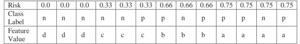
Risk 0.0 0.0 0.0 0.33 0.33 0.33 0.66 0.66 0.66 0.75 0.75 0.75 0.75 Class

Label n n n n n p p n p p p n p Feature

Value d d d c c c b b b a a a a Table 3.3 Negated version of the training dataset. The risk values are calculated again and

instances are sorted in ascending order

3.3 Handling Continuous Features

Having found the necessary and sufficient conditions for the risk function for a categorical feature to result in the maximum possible AUC, the next problem is to determine a mechanism for handling the continuous features. An obvious and trivial risk function maps any real value seen in the training set with the class

27

value p to 1 and any real value with the class value n to 0. This risk function will result in the maximum possible value for AUC, which is 1.0. However, such a risk function will over fit the training data, and will be undefined for unseen values of the feature, which are very likely to be seen in the query instance. So, our first requirement for a risk function for a continuous feature is that it must be defined for all possible values of that continuous feature. A straightforward solution to this requirement is to discretize the continuous feature by grouping all consecutive values with the same class value to a single categorical value; the cut off points can be set to the middle point between feature values of differing class labels. The risk function, then, can be defined using the risk function given in Eq. 3.4 for categorical features. Although this would result in a risk function that is defined for all values of a continuous function, it would still suffer from the over fitting problem. In order to overcome this problem, the REMARC algorithm makes the following assumption:

Assumption 1: The risk values are either non-increasing or non-decreasing for the increasing values of a continuous feature.

Although there exist some features in real-world domains that do not satisfy this assumption, in the datasets we examined this assumption is satisfied in general.

This assumption is also consistent with the interpretations of the values of continuous features in many real-world applications. For example, in a medical domain, a high value of fasting blood glucose is an indication for a high risk of diabetes. On the other hand, low fasting blood glucose is an indication of a risk for another heath problem, called hypoglycemia.

3.3.1 The MAD Method

The REMARC algorithm requires all features to be categorical. Therefore, the continuous features in a dataset need to be categorized. The aim of a

28

discretization method is to find the proper cut-points in order to categorize a given continuous feature. After the discretization process a continuous feature is treated as a discrete feature whose number of intervals is known on the continuous.

The MAD method is designed to maximize the AUC value by checking the ranking quality of values of a continuous feature. The MAD algorithm given in Kurtcephe and Guvenir is defined for multi-class datasets [78]. A special version of the MAD method, called MAD2C and defined for two-class problems, is used in REMARC.

In order to measure the ranking quality of a continuous feature, the instances are sorted in ascending order. Sorting is essential for all discretization methods in order to produce unambiguous intervals. After the sorting operation, feature values are used as hypothetical score values and the ROC graph of the feature is drawn. The AUC of the ROC curve shows the overall ranking quality of the continuous feature. In order to obtain the maximum AUC value, only the points on the convex hull must be selected. The minimum number of points that form the convex hull is found by eliminating the points that cause concavities on the graph. In each pass, the MAD method compares the slopes in the order of the creation of the hypothetical lines, finds the junction points (cut-points) that cause concavities and eliminates them. This process is repeated until there is no concavity on the graph. The points left on the graph are the cut-points, which will be used to discretize the feature.

It has been proven that the MAD method finds the cut-points and the AUC value of the feature independently from the class choice. It is shown that the cut-points found by MAD never separate two consecutive instances of the same class. This is an important property, as it shows that a discretization method works properly. The implementation details, formal proofs and empirical evaluation of MAD can be found in Kurtcephe and Guvenir [78].

29

3.3.2 A Toy Dataset Discretization Example

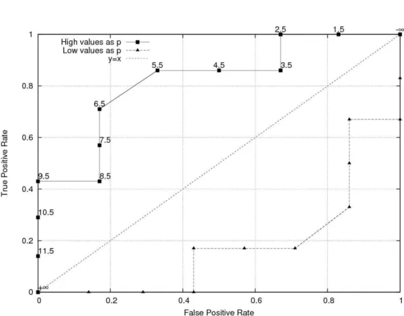
It is possible to visualize the discretization process by using the MAD method. A toy dataset for the discretization is given in Table 3.4. After the sorting operation, the ROC points are formed. This ROC graph is given in Figure 3.3. Since the risk values are either non-increasing or non-decreasing for the increasing values of a continuous feature, two ROC graphs are formed. As can be seen in Figure 3.3 one of these graphs is below the diagonal line since the risk is increasing with increasing values of the continuous feature.

Class

Value n n p n n p n p p n p p p

F1 1 2 3 4 5 6 6 7 8 9 10 11 12

Table 3.4 A toy dataset for visualizing MAD in two-class problems. The name of the attribute to be discretized is F1

30

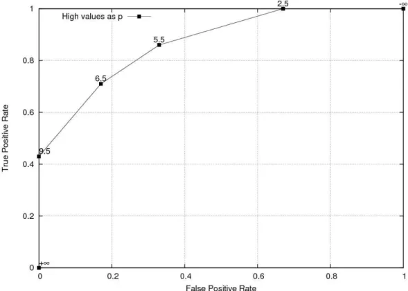
The first pass of the MAD method is shown in Figure 3.4. All points below or on the diagonal are ignored since they have no positive effect on the maximization of AUC. Then the points causing concavities are eliminated. MAD converged to the convex hull in one pass for this example. The points left on the graphs are the discretization cut-points.

Figure 3.4 Final cut-points after the first pass of convex hull algorithm

3.4 REMARC Algorithm

The training phase of the REMARC algorithm is given in Figure 3.5. In the training phase all continuous features are discretized. In order to discretize continuous features, MAD2C, which is shown on the fifth line of Figure 3.5, is used. Risk values are calculated for each value of a given categorical feature (discretized continuous features are included). In this step, the risk function defined in Eq. 3.4 is used in order to obtain the optimal ranking for categorical features. Then, training instances are sorted according to the risk values

31

calculated in the previous step. Since the risk function used by REMARC always results in a convex ROC curve, the AUC is always equal to or greater than 0.5. Therefore, the REMARC algorithm learns a weight wi for a feature fi as

2 * ) 5 . 0 ( − = AUCf w Eq. 3.6

The ROC curve of an irrelevant feature is simply a diagonal line from (0,0) to (1,1), with AUC=0.5. The weight function in Eq. 3.6 assigns 0 to such irrelevant features in order to eliminate them. The risk values and weights of the features are stored for the testing phase.

1 :REMARCTrain (trainSet[M][N]) // Includes M features and N train instances 2 : Begin 3 : for i=0 to M-1 4 : if(isContinuous(trainSet[i])); 5 : cutPoints=MAD2C(trainSet[i][0..N-1]); 6 : numericalValuesToCatVal(cutPoints,trainSet[i]); 7 : risks[i]<-computeCategoricalRisk(trainSet[i][0..N-1]); 8 : sortInstancesByRisk(trainSet[i][0..N-1]); 9 : aucValues[i]<-computeAUC(trainSet[i][0..N-1]); 10: featureWeights[i]=(aucValues[i]-0.5)*2; 11: end 12: end

Figure 3.5 Algorithm of the REMARC method’s training phase.

The testing phase of the REMARC method is straightforward, as for each feature, the risk value corresponding to the value of the feature in the test instance is used. Then the risk of this feature is weighted by its weight, which is calculated in the training phase. The computation of the risk for a query instance

q is in Eq. 3.7. The maximization of AUC for whole dataset is a challenging

problem. Cohen et al. showed that the problem of finding the ordering that agrees best with a learned preference function is NP-Complete [79]. This weighting mechanism is used as a simple heuristic in order to extend this maximization over the whole feature set.

32 risk (q) =

∑

∑

where P(p|qf)is the probability of q being p-labeled, given that the value of feature f in q is qf, and w is the weight of the feature f, calculated by using Eq. f

3.6

Finally, in order to obtain the weighted average, all risk and weight values are summed and final risk is calculated by dividing the cumulative.

1 :REMARCTest (testInstance[M][1]) 2 : Begin

3 : for i=0 to M-1

4 : oneFeatureRisk= risks[i][testInstace[i][0]]; 5 : totalRisk+= oneFeatureRisk * featureWeights[i]; 6 : totalWeight+= featureWeights[i];

7 : end

8 : return totalRisk/totalWeight; 9: end

Figure 3.6 Testing phase algorithm of the REMARC method

The time complexity of the MAD algorithm is given as O(n2), where n is the number of training instances. After discretizing the numerical features the time complexity of the REMARC algorithm is O(m*vlgv+n), where m is the number of features and v is the average number of values per feature. As a result, REMARC is bounded by the MAD algorithm’s time complexity.

3.5 Interpretation of the REMARC Predictive

Model

As mentioned above, the REMARC method does not only provide risk estimation as a single real value, but the predictive model used in order to