Defining the best covariance structure for sequential variation on live weights of Anatolian Merinos male lambs

DEFINING THE BEST COVARIANCE STRUCTURE FOR SEQUENTIAL VARIATION

ON LIVE WEIGHTS OF ANATOLIAN MERINOS MALE LAMBS

H. Orhan, E. Eyduran*_{and Y. Akbaş}**

Süleyman Demirel University, Faculty of Agriculture, Department of Animal Science, 32260, Isparta-TURKEY *_{Igdir University, Faculty of Agriculture, Department of Animal Science, 76000, Iğdır-TURKEY} **_{Ege University, Faculty of Agriculture, Department of Animal Science, Bornova, 35100 İzmir-TURKEY}

Corresponding author email:hikmetorhan@hotmail.com

ABSTRACT

In a repeated measures design with two factors, between-subjects and within-subjects, the most appropriate (univariate or multivariate) method and the best covariance structure explaining sequential variation in live weights of Anatolia Merinos lambs fed with different rations were estimated. In general linear mixed model, univariate ANOVA, Geisser-Greenhouse and Huynth-Feldt epsilon were used as univariate methods while profile analysis as well as mixed model methodology were applied as multivariate methods. The data were composed of twenty-four Anatolia Merinos male lambs with weaning age of 2-2.5 months randomly selected from Polatli State Farm and divided equally into four groups. Rations were mas hor pelletted using molasses, lignobond and aquacup binders. Live weights were measured at six times during experimental period (day 0, 14, 28, 42, 56 and 70). In general linear mixed model, nine covariance structures (CS, CSH, UN, HF, AR(1), ARH(1), ANTE(1), TOEP and TOEPH) were applied. AIC, AICC and SBC criteria were used to detect the best defining covariance structure for fitting data. The best covariance structure for the data set was found to be Unstructured (UN). In the case of violation of spherity assumption, using mixed model approach was advised according to AIC, AICC and SBC criteria. As a conclusion, in repeated measures design use of mixed model methodology was recommended to determine the best covariance structure for defining experimental data sets. Key words: Repeated Measures Design, Univariate ANOVA, Profile Analysis, General Linear Mixed Model(GLM).

INTRODUCTION

Repeated measures are consecutive data obtained over time from the same experimental units such as people, plant and animals. Repeated measures designs have commonly used in animal science (Littell et al., 1996); Akbaş et al., 2001). The most popular repeated measures design with two factors, treatment (between-subject) and time (within-(between-subject) is analogous to split-plot experiment design (Littell et al., 1996). Two-way ANOVA are simply used for analyzing experiments with two factors (Ergun and Aktas, 2009). Repeated ANOVA is applied traditionally for statistical analysis of data including between-subject and within-subject factors. Repeated ANOVA is used safely when spherity assumption is provided (Eyduran and Akbaş, 2010). The sphericity assumption is an assumption about the structure of the covariance matrix in a repeated measures design. Sphericity relates to the equality of variances of differences between levels of the repeated measures. Mauchly’s test can be used to control Sphericity assumption.

When this assumption is invalid, Greenhouse-Geisser epsilon (G-G) adjusted F test, Huynh-Feldt epsilon (H-F) adjusted F test, profile analysis (Repeated MANOVA) and mixed model are used in repeated measures designs. It was stated that multivariate methods

gave more reliable results than univariate methods (Keselman et al., 1993); Algina and Oshima, 1994); Tabachnick and Fidel (2001); Gürbüz et al. (2003). Eyduran et al. (2008) reported that profile analysis was more informative than repeated ANOVA.

Since data with no missing observations are used in repeated ANOVA, experimental units with missing observations are deleted in traditional repeated and profile analysis. However, mixed model methodology for repeated measures design is used straightforwardly for data with or without missing observations (Eyduran and Akbaş, 2010).

Mixed model methodology enable statisticians to specify different covariance structures in repeated mesures designs where both random and fixed effects are included in the model. Therefore, mixed model methodology are potentially the most powerful tool.

Although reports on application of mixed model methodology in animal science without specifying various covariances are available (Pancarci et al., 2007; 2009), however, reports on jointly usage possibilities of univariate ANOVA, profile analysis, mixed model approaches (with different covariance structure) in repeated measures design in animal science are few in literature (Littell et al., 1998; Akbaş et al., 2001) and getting more importance.

In animal nutrition trials, the most appropriate covariance structure defining consecutive changes on fattening performance of animals over time within ration groups using mixed model methodology should be determined. Hence, the aims of this study were to examine the performances of univariate and multivariate methods and determine the most appropriate covariance structures for defining sequential variation on live weights of Anatolia Merinos male lambs over fattening period.

MATERIALS AND METHODS

In this study, twenty-four Anatolia Merinos male lambs with weaning age of 2-2.5 months randomly selected from Polatli State Farm and randomly divided into four groups Gürbüz (1999). There are four levels of ration; one is mash (M) and three pelletted rations formed using molasses (Mo), lignobond (L) and aquacup binders (A) with six replicates. Live weights were measured at six times (day 0, 14, 28, 42, 56 and 70).

First, One-way ANOVA was applied and Levene’s test for homogeneity of variance was used for each period (Ayhan et al., 2008).

Repeated measure design with two factors, ration (between-subject) and time (within-subject) was fitted to data. Greenhouse-Geisser Epsilon (G-G) and Huynh-Feldt Epsilon (H-F) adjusted F test approaches were traditionally used when spherity assumption for univariate approach is violated (Keskin and Mendeş, 2001). However, using these two approaches presents not an optimal solution. Mixed model methodology is a statistical tool that has computational advantages in repeated measures design (Baguley, 2004). For instance, when validity of the spherity assumption is violated, mixed model methodology allow statisticians to specify different covariance structures for data with/without missing observations and were more superior to univariate methods, which are based on only unstructured (UN) covariance structure (Littell et al., 1996).

The statistical model is:

 

Y

 

  













e

i: i th fixed level of ration (treatment) factor

( )

j i



: the random effect of j. animal (experimental unit) fed with i. ration

_k: k th fixed time effect,

()ik: Ration by time interaction effect, eijk: Random error element.

Matrix notation of the model was Y = Xβ + Zu + e where β and u are vectors for fixed (ration, time and ration by time interaction) and random (individual within

ration) effects, respectively; X and Z are the design matrices for the corresponding fixed and random effects. Assumptions are: u is MVN(0, G), random error term e is MVN(0, R) and V(Y) = ZGZ’ + R. General linear mixed model can be fit using SAS package program with MIXED procedure using RANDOM command to generate G matrix, whereas REPEATED command controls R matrix, which is connected to variation within experimental unit (Akbaş et al., 2001). Statistical analysis were carried out using GLM and MIXED procedures of SAS. DDFM option on the model statement in MIXED procedure was used to specifiy containment, Satterthwaite or Kenward Roger approaches for determining fixed effects and degrees of freedom. Containment approach is default in MIXED procedure.

Akaiki’s Information Criterion (AIC), Burnham-Handerson Criterion (AICC) and Shwartz’s Bayesian Criterion (SBC) were used to determine the most suitable covariance structure for mixed model approach in repeated measures design. The covariance structure given the AIC, AICC and SBC values which is the most closest to zero is accepted as the best covariance structure. The smaller the fit criteria is the better the covariance structure in SAS. Compared covariance structures in mixed model are: First- Order Autoregressive (AR(1)), Heterogenous First-Order Autoregressive (ARH(1)), First-Order Ante-Dependence(ANTE(1)), Compound Symmetry (CS), Unstructured (UN), Huynth-Feldth (HF), Heterogenous Compound Symmetry (CSH), Toeplitz

(TOEP), Heterogenous Toeplitz (TOEPH).

Comprehensive information on these covariance structures were given in Littell et al. (1996). Produced outputs from MIXED procedure of SAS program interpreted as “smaller is better”.

RESULTS AND DISCUSSION

Descriptive statistics of live weights measured at each period are presented as mean ± standard error in Table 1. Probabilities of Levene’s test for homogeneity of variances on live weights measured at each time period were found more than 5% level (data not shown). Homogeneity of variance assumption, one of the basic assumptions of one way-ANOVA, was provided for each period.

Means among periods(times) were changed from 22.48 to 38.35 kg for mash ration, from 23.65 to 41.31 kg for molasses ration, from 23.41 to 41.34 for lignobond ration, and from 22.83 to 41.56 for aquacup ration, respectively. Kolmogorov-Smirnow normality test results for live weight data at each time period showed that normality assumption was provided at each period. The effect of ration on live weight at each period was non-significant (P>0.05).

Probability of Mauchly’s test for spherity assumption was significant(P<0.001). This means that

multivariate approach should be prefferred instead of univariate approach. Within subjects effects were results are given in Table 4. Greenhouse-Geisser (G-G) and Huynh-Feldt (H-F) Epsilon adjusted F test approaches can practically use when validity of spherity assumption was not provided. However, these two approaches can not present optimal solutions. When these two approaches were taken into consideration, time effect was also significant (P<0.001).

Profile analysis (Repeated MANOVA), multivariate approach to repeated measures design is one

of the most noteworthy multivariate approaches. Results on time, ration and ration by time effects are presented in Table 5-7. As seen from Table 5, null hypothesis on the time effect (called flatness test) was rejected at 1 % level. Time was also a significant effect in profile analysis. No significant effects of ration (Coincident test) and ration by time interaction (Parallel test) were found in profile analysis (Table 6 and 7). Differences among ration averages were not varied considerably from time to time. Table 1. Mean ± SE of live weights of Anatolia Merinos lambs for the rations at each time

Time (day) N Mash Molasses Lignobond Aquacup Probability*

0 6 22.48±0.60 23.65±0.44 23.41±0.47 22.83±0.35 P>0.05 14 6 26.48±1.00 27.70±0.52 26.95±1.40 27.02±0.67 P>0.05 28 6 30.63±0.86 31.86±0.58 30.78±2.09 31.32±0.60 P>0.05 42 6 33.48±1.10 35.05±0.87 35.08±0.73 34.63±0.52 P>0.05 56 6 36.35±1.04 38.63±1.06 39.61±0.77 39.48±0.68 P>0.05 70 6 38.35±1.11 41.31±1.12 41.34±0.91 41.56±0.58 P>0.05

*: F test statistics significant levels for ration factor in each control time

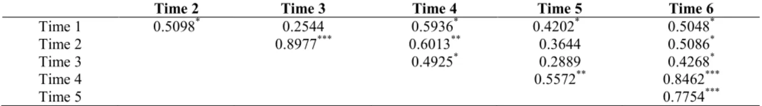
Pearson’s correlation coefficients among repeated live weights are given Table 2. All the Pearson’s correlation coefficients were positive, but some of them were statistically significant. The highest correlations between time2 – time3, time4 – time6, and time5 – time6 were detected (P<0.001).

Table 2. Pearson’s correlation coefficients between repeated live weights

Time 2 Time 3 Time 4 Time 5 Time 6

Time 1 0.5098* _{0.2544 0.5936}* _0.4202*_{* 0.5048}* Time 2 0.8977*** _0.6013** _{0.3644 0.5086}* Time 3 0.4925* _{0.2889 0.4268}* Time 4 0.5572** _0.8462*** Time 5 0.7754*** * P<0.05 **P <0.01 ***P<0.001

Univariate ANOVA results in split plot design is partially given in Table 3 with command statements used in PROC GLM of SAS. Under this case, ration by time interaction was found non-significant, it is concluded that correlations between pairs of measurements as well as variances of mesurements at all times are equal. Only time effect was significant (P<0.001).

Table 3. Result of Univariate ANOVA obtained from Split plot design

Source of Variation DF MS F Probability

Ration 3 23.545943 1.35 0.2879 Individual(ration) 20 17.500064 Time 5 1089.0831 432.59 <0.0001 Ration x Time 15 2.535143 1.01 0.4544 Error 100 2.517602 PROC GLM;

CLASS RATION INDIVIDUAL TIME;

MODEL WEIGHT = RATION INDIVIDUAL(RATION) TIME RATION*TIME; RANDOM INDIVIDUAL(RATION)/ TEST;

LSMEANS RATION / STDERR E=INDIVIDUAL(RATION); LSMEANS RATION*TIME / PDIFF;

RUN;

“PRINTE” option in REPEATED statement of PROC GLM is defined to evaluate validity of Spherity assumption with the following statements:

PROC GLM; CLASS RATION;

MODEL TIME1 TIME2 TIME3 TIME4 TIME5 TIME6 = RATION; REPEATED TIME 6 (1 2 3 4 5 6)/SUMMARY PRINTE;

RUN;

Table 4. Results of within subjects effects Source of Variation df Type III

Sum of Sq. SquareMean F P G– GAdjusted Pr > FH – F

Time 5 5445.4156 1089.0831 432.59 <.0001 <0.0001 <0.0001

Time x Ration 15 38.0271 2.5351 1.01 0.4544 0.4418 0.4418

Error (Time) 100 251.7602 2.5176

Greenhouse-Geisser Epsilon : 0.5289 Huynh-Feldt Epsilon: 0.7084

Information criteria for different covariance structures in mixed model approach are summarized in Table 8. According to AIC, AICC, and SBC fitting criteria, unstructured (UN) was the best covariance structure while the worst one was compound symmetry (CS). UN gave information about growth-development mechanism and consecutive variation at fattening

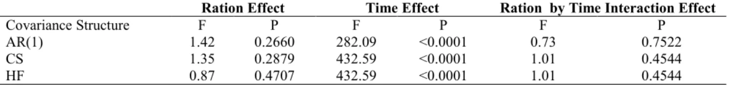
performances of Anatolia Merinos lambs over trial time. Results could not be obtained for ARH(1), ANTE(1), CSH, and TOEPH covariance structures (data not shown). As can be seen in Table 9, only time effect was statistically significant (P<0.001) in mixed model analysis.

Table 5. Flatness (time effect) test results

Statistics Value F Numerator Df Deminator Df P

Wilks' Lambda 0.00999188 317.06 5 16 <.0001

Pillai'sTrace 0.99000812 317.06 5 16 <.0001

Hotelling L. Tr. 99.08124033 317.06 5 16 <.0001

Roy's Gr. Root 99.08124033 317.06 5 16 <.0001

Table 6. ANOVA table of combining ration or time effect (coincident)

Source of Variation Df Sum of Squares Mean Squares F P

Between Ration 3 70.6378293 23.5459431 1.35 0.2879

Error 20 350.0012774 17.5000639

Table 7. Parallel test results (Ration by Time interaction)

Statistics Value F Numerator Df Deminator Df P

Wilks' Lambda 0.58432687 0.64 15 44.57 0.8270

Pillai's Trace 0.45533540 0.64 15 54 0.8248

Hotelling L. Tr. 0.64441177 0.65 15 25.399 0.8037

Roy's Gr. Root 0.52104387 1.88 5 18 0.1488

Table 8. Fitting criteria results for comparing covariance structures

Covariance Structure

AR(1) CS HF TOEP UN

Akaiki Information Criterion (AIC) 531.8 539.1 527.8 537.0 506.8

Burnham-Handerson Criterion (AICC) 532.0 539.3 528.8 537.7 517.3

Shwartz’s Bayes Criterion ( SBC) 535.4 542.7 536.0 544.0 532.8

Table 9. Significance results of fixed effects in mixed model approach (F and P values)

Ration Effect Time Effect Ration by Time Interaction Effect

Covariance Structure F P F P F P

AR(1) 1.42 0.2660 282.09 <0.0001 0.73 0.7522

CS 1.35 0.2879 432.59 <0.0001 1.01 0.4544

TOEP 1.41 0.2687 298.26 <0.0001 0.74 0.7374

UN 1.35 0.2879 396.33 <0.0001 0.86 0.6106

Univariate ANOVA, Geisser-Greenhouse Epsilon and Huynth-Feldt Epsilon, profile analysis and mixed model approach were discussed with a model including two factors, ration and time. In event of violation of spherity assumption, advantages of mixed model approach were also tested. Among within-subject effects, ration, time and ration by time interaction effects were examined. Repeated measures design with two factors, between-subjects (ration) and with-between-subjects (time) has been extensively used. With violation of Spherity assumption, the use of univariate ANOVA may produce indefinable interpretations as mentioned by numerous authors (Algina and Oshima, 1994; Tabachnick and Fidel, 2001; Gürbüz et al., 2003; Eyduran et al., 2008). When Spherity assumption was invalid, it was reported that use of Greenhouse-Geisser Epsilon (G-G) and Huynh-Feldt Epsilon (H-F) approaches as an alternative was routinely more suitable than that of univariate ANOVA. However, when the assumption was provided, univariate ANOVA was reported to be more robust than multivariate approaches (Morrison, 1990; Movenon et al., 2007).

Using profile analysis as the second alternative may be recommended when number of experimental units (subjects) in each level of independent variable (ration) is more than number of time levels (Tabachnick and Fidel, 2001). In the current study, number of animals for each ration is equal to level of time effects. In this case, power of profile analysis would be expected to be lower.

In recent years, use of mixed model methodology in repeated mesures design have been preffered by some authors (Pancarci et al., 2007; 2009; Eyduran and Akbaş, 2010).

It was reported that the mixed model approach gave more reliable results than univariate ANOVA, Greenhouse-Geisser Epsilon (G-G), Huynh-Feldt Epsilon (H-F) and Profile Analysis as in the current study (Littell

et al., 1996; 1998; Akbaş et al., 2001). The mixed model

approach may also be used easily for data set including missing observations. On the other hand, univariate ANOVA, Greenhouse-Geisser (G-G), Huynh-Feldt (H-F) epsilon and profile analysis are never routinely used for analyzing data set with missing observations (Littell et

al., 1996; Eyduran and Akbaş, 2010). This is one of the

most important advantage of mixed model approach in repeated measurement design. Unlike others, mixed model approach helps researchers to determine the most appropriate covariance structure for data set with/without missing observations.

Conclusions: In the current study, performances of univariate (univariate ANOVA, Greenhouse-Geisser (G-G), Huynh-Feldt (H-F) epsilon) and multivariate

approaches (Profile analysis and mixed model approach) were compared with each other.

 The effect of ration factor on fattening performances of Anatolia Merinos lambs was non-significant but the effect of time was significant. Unstructured (UN) was the best covariance structure defining growth-development mechanism or consecutive variation at fattening performances of Anatolia Merinos lambs over experimental periods.

 In the case of violation of spherity assumption, usage of mixed model approaches was appropriate than those of univariate ANOVA, Geisser-Greenhouse Epsilon, Huynh-Feldt Epsilon, and Profile Analysis. Also, mixed model approach in repeated measures design allow researchers to specify suitable covariance structures for used data.

 Determination of the most appropriate covariance structure in repeated mesuares design provides to estimate reliably within subjects effects (fixed effects). Thus, mixed model approach permits us to use different covariance options.

 Mixed model approaches could be used for data set with missing observations. Whereas, univariate approaches and profile analysis are never applied for data sets having missing observations. This is one of the most important advantage of mixed model approach in repeated measures design.

 Mixed model approaches specified with different covariance structures are recommended because various covariance structures in univariate ANOVA, G-G, H-F, and profile analysis are never specified. Acknowledgement: We would like to express our thanks to Dr. Yavuz Gürbüz giving his PhD thesis data for interpretation of alternative statistical techniques.

REFERENCES

Akbaş Y., M. Z. Fırat and Ç. Yakupoğlu (2001). Comparison of Different Models Used in the Analysis of Repeated Measurements in Animal Science and Their SAS Applications. Agricultural Information Technology Symposium, Sütçü İmam University, Agricultural Faculty, Kahramanmaraş, 20-22 September 2001.

Algina J. and T. C. Oshima (1994). Type I error rates for Huynh’s General Approximation and Improved General Approximation tests. British J. Math. and Stat. Psychology (BJMSP), 47: 151-165. Ayhan V., I. Diler, M. Arabaci and H. Sevgili (2008).

Enzyme Supplementation to Soybean Based Diet in Gilthead Sea Bream (Sparus Aurata): Effects

on Growth Parameters and Nitrogen and Phosphorus Excretion. Kafkas Univ. J.Vet.Faculty.14(2):161-168.

Baguley T: (2004). An introduction to sphericity. http: // homepages. gold. ac. uk/ aphome/ spheric.html. Ergun G,. and S. Aktas (2009). Comparisons of sum of

squares methods in ANOVA Models. Kafkas Univ. J. Vet. Faculty. 15(3): 481-484.

Eyduran E, K. Yazgan and T. Özdemir (2008). Utilization of profile analysis in animal science. J. Anim. and Vet. Advances, 7(7):796-798. Eyduran, E. and Y. Akbaş (2010). Comparison of

diıfferent covariance structure used for experimental design with repeated measurement. J. Anim. and Plant Sci., 20(1): 44-51.

Gürbüz F., E. Başpınar, H. Çamdeviren and S. Keskin (2003). Analyzing experimental designs with repeated measurement. Yuzuncu Yil University. Publishing No: 130, Van.

Gürbüz Y. (1999). A Research using the effects of different pellet binders on the pellet quality and fattening performance and carcass yield the lambs fattening rations. PhD thesis. Ankara Univ. Instutude of Science. Ankara.

Keselman H. J., K. C. Carriere and L. M. Lix (1993). Testing repeated measures hypotheses when covariance matrices are heterogeneous. J. Educ. Stat., 18(4): 305-319.

Keskin S. and M. Mendeş (2001). Experimental Designs including repeated measurement in one’s levels of their factors. S.Ü. J. Agricultural Faculty, 15(25): 42-53.

Littell R. C., P. R. Henry and C. B. Ammerman (1998). Statistical analysis of repeated measures data using SAS procedures. J. Anim. Sci., 76(4): 1216-1231.

Littell R. C., G. A. Milliken, W. W. Stroup and R. D. Wolfinger (1996). SAS System for Mixed Models, Cary, NC: SAS Institute Inc.

Morrison D. F. (1990). Multivariate statistical methods (3rd ed.). New York: McGraw-Hill.

Movenon S. W., M. A. Betz, K. Wang, and B. Zumbo (2007). Application of a New Procedure for Power Analysis and Comparison of the Adjusted Univariate and Multivariate Tests in Repeated Measures Designs. J. Mod Appl Stat Meth, 6(1):36-52.

Pancarci S. M., K. Gurbulak, H. Oral, M. Karapehlivan, R. Tunca and A. Çolak (2009). Effect of Immunomodulatory Treatment with Levamisole on Uterine Inflammation and Involution, Serum Sialic Acid Levels and Ovarian Function in Cows. Kafkas Univ. J. Vet. Faculty. 15(1): 25-33.

Pancarci S. M., C. Kacar, M. Ogun, O. Gungor, K. Gurbulak, H. Oral, M. Karapehlivan and M. Citil (2007). Effect of L-Carnitine Administration on Energy Metabolism During Peripaturient Periodin Ewes. Kafkas Univ. J. Vet. Faculty. 13(2): 149-154.

Tabachnick B. G. and L. S. Fidel (2001). Using Multivariate Statistics. Allyn& Bacon, USA.