JHEP05(2012)128
Published for SISSA by Springer
Received: March 20, 2012 Revised: April 17, 2012 Accepted: May 2, 2012 Published: May 28, 2012
Jet mass and substructure of inclusive jets in
√
s = 7 TeV pp collisions with the ATLAS experiment
The ATLAS collaboration
Abstract: Recent studies have highlighted the potential of jet substructure techniques to identify the hadronic decays of boosted heavy particles. These studies all rely upon the assumption that the internal substructure of jets generated by QCD radiation is well understood. In this article, this assumption is tested on an inclusive sample of jets recorded with the ATLAS detector in 2010, which corresponds to 35 pb−1 of pp collisions delivered by the LHC at √s = 7 TeV. In a subsample of events with single pp collisions, measure-ments corrected for detector efficiency and resolution are presented with full systematic uncertainties. Jet invariant mass, kt splitting scales and N -subjettiness variables are
pre-sented for anti-kt R = 1.0 jets and Cambridge-Aachen R = 1.2 jets. Jet invariant-mass
spectra for Cambridge-Aachen R = 1.2 jets after a splitting and filtering procedure are also presented. Leading-order parton-shower Monte Carlo predictions for these variables are found to be broadly in agreement with data. The dependence of mean jet mass on additional pp interactions is also explored.
JHEP05(2012)128
Contents
1 Introduction 1
2 Definitions 2
2.1 Jet algorithms 2
2.2 The splitting and filtering procedure 3
2.3 ktsplitting scales, pdij 4
2.4 N -subjettiness 4
3 The ATLAS detector 5
4 Dataset and reconstruction 5
5 Monte Carlo samples 6
6 Detector-level distributions 7
7 Systematic uncertainties 7
8 Data correction 12
9 Results 12
10 Mean mass with multiple proton-proton interactions 15
11 Conclusions 19
The ATLAS collaboration 25
1 Introduction
The ATLAS experiment observes proton-proton (pp) collisions provided by the Large Hadron Collider (LHC). The outcome of these collisions is frequently the production of large numbers of hadrons. In order to understand these collisions, studies usually group hadrons into jets defined by one of a number of standard algorithms [1–7]. The variables most often used in analyses are the jet direction and momentum transverse to the beam (pT). However the jets remain composite objects and their masses and internal substructure
contain additional information.
One strong motivation for studies of the internal substructure of jets is that at the LHC particles such as W and Z bosons and top quarks are produced abundantly with significant Lorentz boosts. The same may also be true for new particles produced at the LHC. When
JHEP05(2012)128
such particles decay hadronically, the products tend to be collimated in a small area of the detector. For sufficiently large boosts, the resulting hadrons can be clustered into a single jet. Substructure studies offer a technique to extract these single jets of interest from the overall jet background. Such techniques have been found promising for boosted W decay identification, Higgs searches and boosted top identification amongst others [8]. However, many of these promising approaches have never been tested with collision data and rely on the assumption that the internal structure of jets is well modelled by parton-shower Monte Carlo approaches. It is therefore important to measure some of the relevant variables in a sample of jets to verify the expected features.
In this paper, measurements are made with an inclusive sample of high-transverse momentum jets produced in proton-proton collisions with a centre-of-mass energy (√s) of 7 TeV. This is a natural continuation of the studies in previous experiments [9–13]. It also complements previous ATLAS studies [14] probing the shape of jets reconstructed with the anti-ktalgorithm [5] with smaller radius parameters R = 0.4 and 0.6.
This study focuses on two specific jet algorithms that are likely to be of interest for future searches: anti-kt jets with an R-parameter of 1.0 and Cambridge-Aachen [3,4] jets
with R = 1.2. Jets are required to be at high-transverse momentum (pT > 200 GeV)
and central in rapidity1 (|y| < 2). The normalised cross-section as a function of jet mass, taken from the jet four-momentum, is measured for both these algorithms. In addition to the mass, two sets of substructure variables, kt splitting scales [15] and N -subjettiness
ratios [16], are measured. For the Cambridge-Aachen jets, the mass distribution after a substructure splitting and filtering procedure [17] is also presented.
2 Definitions
2.1 Jet algorithms
Jets are constructed using two infrared and collinear-safe recombination jet algorithms, anti-kt and Cambridge-Aachen, as implemented in the FastJet package [18]. Both act
by iteratively merging the nearest objects in the event but with different definitions of “distance”. The anti-kt jet algorithm builds jets with a very regular shape, while the
Cambridge-Aachen algorithm builds less regular jets. This analysis uses R-parameters of 1.0 and 1.2, for anti-kt and Cambridge-Aachen jets respectively, in line with recent studies
of heavy boosted objects. All discussion of jet algorithms in this paper assumes that the constituents from which the jet is composed are recombined using four-vector addition. Jets in the real or simulated detector are constructed from clusters of energy deposited in the calorimeter (see section4). Jets in the “true” final state, or “hadron level”, are defined as jets made from all particles with a proper lifetime longer than 10 ps, including neutrinos.
1
ATLAS uses a right-handed coordinate system with its origin at the nominal interaction point (IP) in the centre of the detector and the z-axis along the beam pipe. The x-axis points from the IP to the centre of the LHC ring, and the y-axis points upward. Cylindrical coordinates (r, φ) are used in the transverse plane, φ being the azimuthal angle around the beam pipe. The pseudorapidity is defined in terms of the polar angle θ as η = − ln tan(θ/2). Rapidity is y = 1/2 × ln((E + pz)/(E − pz)).
JHEP05(2012)128
2.2 The splitting and filtering procedure
The “splitting and filtering” procedure aims to identify relatively hard, symmetric splittings in a jet that contribute significantly to the jet’s invariant mass. This procedure is taken from recent Higgs search studies [17,19]. The parameters are tuned to maximise sensitivity to a Standard Model Higgs boson decaying to b¯b, but this procedure is suitable generally for identifying two-body decay processes. The effect of the procedure is to search for jets where clustering the constituents with Cambridge-Aachen combines two relatively low mass objects to make a much more massive object. This indicates the presence of a heavy particle decay. The procedure then attempts to retain only the constituents believed to be related to the decay of this particle. Because the procedure itself uses the Cambridge-Aachen algorithm, it is most natural to apply it to jets originally found with this algorithm.
Each stage in the clustering combines two objects j1 and j2 to make another object j.
Use definitions v = min(p
2 T j1,p2T j2) m2 j δR2j1,j2 and δRj1,j2= q
δy2j1,j2+ δφ2j1,j2, where δy and δφ
are the differences in rapidities and azimuthal angles respectively. The procedure takes a jet to be the object j and applies the following:
1. Undo the last clustering step of j to get j1 and j2. These are ordered such that
their mass has the property mj1 > mj2. If j cannot be unclustered (i.e. it is a single
particle) or δRj1,j2< 0.3 then it is not a suitable candidate, so discard this jet.
2. If the splitting has mj1/mj < µ (large change in jet mass) and v > vcut (fairly
symmetric) then continue, otherwise redefine j as j1 and go back to step 1. Both µ
and v are parameters of the algorithm.
3. Recluster the constituents of the jet with the Cambridge-Aachen algorithm with an R-parameter of Rf ilt= min(0.3, δRj1,j2/2) finding n new subjets s1, s2. . . snordered
in descending pT.
4. Redefine the jet as the sum of subjet four-momentaPmin(n,3)
i=1 si.
The algorithm parameters µ and vcutare taken as 0.67 and 0.09 respectively [19].
The µ cut attempts to identify a hard structure in the distribution of energy in the jet, which would imply the decay of a heavy particle. The cut on v further helps by suppressing very asymmetric decays of the type favoured by splittings of quarks and gluons. A notable modification of the original procedure [17] in this paper is the addition of the δRj1,j2 cut
in step 1. This cut is applied because with current techniques the correction for detector resolution at angular scales below 0.3 is not well controlled. Steps 3 and 4 filter out some of the particles in the candidate jet, the aim being to retain particles relevant to the hard process while reducing the contribution from effects like underlying event and pile-up. The 4-vector after step 4 can be treated like a new jet. This new jet has a pT and mass less
JHEP05(2012)128
2.3 kt splitting scales, pdij
The kt splitting scales are defined by reclustering the constituents of the jet with the kt
recombination algorithm [1,2]. The kt-distance of the final clustering step can be used to
define a splitting scale variable√d12:
p
d12= min(pT j1, pT j2) × δRj1,j2,
where 1 and 2 are the two jets before the final clustering step [15]. The ordering of clustering in the ktalgorithm means that in the presence of a two-body heavy particle decay the final
clustering step will usually be to combine the two decay products. The parameter√d12can
therefore be used to distinguish heavy particle decays, which tend to be more symmetric, from the largely asymmetric splittings of quarks and gluons. The expected value for a heavy particle decay is approximately m/2, whereas inclusive jets will tend to have values ∼ pT/10, although with a tail extending to high values. The variable √d23 is defined
analogously but for the two objects combined in the penultimate clustering step.
2.4 N -subjettiness
The N -subjettiness variables τN [16] are designed to be smooth, continuous observables
related to the subjet multiplicity. Intuitively, the variables can be thought of as answering the question: “How much does this jet look like N different subjets?” The variable τN
is calculated by clustering the constituents of the jet with the kt algorithm and requiring
N subjets to be found. These N subjets define axes within the jet around which the jet constituents may be concentrated. The variables τN are then defined as the following sum
over all constituents k of the jet: τN = 1 d0 X k pT,k× min(δR1,k, δR2,k, . . . , δRN,k) (2.1) d0 = X k pT ,kR, (2.2)
where δRi,k is the distance from the subjet i to the constituent k and R is the R-parameter
of the original jet algorithm.
Using this definition, τN describes how well the substructure of the jet is described by
N subjets by assessing the degree to which constituents are localized near the axes defined by the ktsubjets. For two- and three-body decays, respectively, the ratios τ2/τ1 and τ3/τ2
have been shown to provide excellent discrimination for hadronic decays of W -bosons and boosted top quarks [20]. These ratios will be referred to as τ21 and τ32 respectively. These
variables mostly fall within the range 0 to 1. As an example, τ21 ' 1 corresponds to a
jet which is narrow and without substructure; τ21 ' 0 implies a jet which is much better
described by two subjets than one. Similarly low values of τ32 imply a jet which is much
better described by three subjets than two. However, as can be seen from the definition, adding an additional subjet axis will tend to reduce the value of τN and therefore even
JHEP05(2012)128
3 The ATLAS detector
The ATLAS detector [21] provides nearly full solid angle coverage around the collision point with tracking detectors, calorimeters and muon chambers. Of these subsystems the most relevant to this study are the inner detector, the barrel and endcap calorimeters, and the trigger system.
The inner detector is a tracking detector covering the range |η| < 2.5 and with full coverage in φ. It is composed of a silicon pixel detector, a silicon microstrip detector and a transition radiation tracker. The whole system is immersed in a 2 T magnetic field. The information from the inner detector is used to reconstruct tracks and vertices.
The barrel and endcap calorimeters cover the regions |η| . 1.5 and 1.5 . |η| < 3.2, respectively. Electromagnetic measurements are provided by a liquid-argon (LAr) sampling calorimeter. The granularity of this detector ranges from δη×δφ = 0.025×0.025 to 0.1×0.1. Hadronic calorimetry in |η| < 1.7 is provided by a scintillating-tile detector, while in the endcaps, coverage is provided by a second LAr system. The granularity of the hadronic calorimetry ranges from 0.1 × 0.1 to 0.2 × 0.2.
The trigger system [22] is composed of three consecutive levels. Only the Level-1 (L1) trigger is used in this study, with higher levels not rejecting any events. The L1 trigger is based on custom-built hardware that processes events with a fixed latency of 2.5 µs. Events in this analysis are selected based on their L1 calorimeter signature. The L1 calorimeter trigger uses coarse detector information to identify interesting physics objects above a given transverse energy (ET) threshold. The jet triggers use a sliding window algorithm taking
square δη × δφ = 0.2 × 0.2 jet elements as input. The window size is 0.8 × 0.8.
4 Dataset and reconstruction
The data analysed here come from the 2010√s = 7 TeV pp dataset. Data are used in this study only if the detector conditions were stable, there was a stable beam present in the LHC, the luminosity was reliably monitored and the trigger was operational. The selected data set corresponds to an integrated luminosity of 35.0 ± 1.1 pb−1 [23,24].
Events in this analysis are first selected by the L1 calorimeter trigger system. The efficiency of this trigger was evaluated in data and found to contain no significant biases for the selection used here. For the lowest pT bin (200–300 GeV) a trigger is used which
was only available for part of the dataset. As a result some plots are presented with the lower integrated luminosity of 2.0 ± 0.1 pb−1.
To reject events that are dominated by detector noise or non-collision backgrounds, events are required to contain a primary vertex consistent with the LHC beamspot, recon-structed from at least five tracks with pT> 150 MeV. Additionally, jets are reconstructed
with the anti-kt algorithm using an R-parameter of 0.6. Events are discarded if any such
jet with transverse momentum greater than 30 GeV fails to satisfy a number of quality cri-teria, including requirements on timing and calorimeter noise [25]. This selection removes approximately 3% of events in this dataset.
JHEP05(2012)128
Additional proton-proton collisions (pile-up) can have a significant impact on quantities like jet mass and substructure [8]. The primary results in this paper are therefore presented only in events where the number of reconstructed primary vertices (NPV) composed of at
least five tracks is exactly one. This requirement selects approximately 22% of events in the 2010 dataset. As vertex finding is highly efficient, this approach is expected to be very good at rejecting pile-up, and no additional systematic uncertainties as a result of this requirement are considered. The effects of pile-up are discussed in more detail in section10. Calorimeter cells are clustered using a three-dimensional topological algorithm. These clusters provide a three-dimensional representation of energy depositions in the calorimeter with a nearest neighbour noise suppression algorithm [26]. The resulting clusters are made massless and then classified as either electromagnetic or hadronic in origin based on their shape, depth and energy density. Cluster energies are corrected with calibration constants, which depend on the cluster classification to account for calorimeter non-compensation [25]. The clusters are then used as input to a jet algorithm.
As part of this study, specific calibrations for these jet algorithms have been devised. Calibrations for the mass, energy and η of jets are derived from Monte Carlo (specifically Pythia [27]). Hadron-level jets (excluding muons and neutrinos) are matched to jets re-constructed in the simulated calorimeter. The matched pairs are used to define functions for these three variables, dependent on energy and η, which on average correct the recon-structed quantities back to the true scale. This correction is of the order 10-20% for mass and energy and 0.01 for η.
Jets constructed from tracks are used for systematic studies in this paper. These track-jets are constructed using the same algorithms as calorimeter track-jets. The input constituents are inner-detector tracks originating only from the selected pp collision of interest as selected by the criteria pT > 500 MeV, |η| < 2.5, |z0| < 5 mm and |d0| < 1.5 mm [28]. Here z0 and
d0 are the longitudinal and transverse impact parameter of the track at closest approach
to the z-axis, relative to the primary vertex.
The measurements presented in this paper are for jets that have |y| < 2 in four 100 GeV pT bins spanning 200 to 600 GeV. This selection is not biased by trigger effects and the jets
it selects are contained entirely within the barrel and end-cap subdetectors.
5 Monte Carlo samples
Samples of inclusive jet events were produced using several Monte Carlo (MC) generators including Pythia 6.423 [27] and Herwig++ 2.4 [29]. These programs implement leading-order (LO) perturbative QCD (pQCD) matrix elements for 2 → 2 processes. Additionally, Alpgen 2.13 [30] and Sherpa 1.2.3 [31] are used for some cross-checks. Sherpa and Alpgen implement 2 → n processes such as explicit QCD multijet production. Parton-showers are calculated in a leading-logarithm approximation. Showers are pT ordered in
Pythia and angular ordered in Herwig++. Fragmentation into particles is implemented in Pythia following the string model [32] and in Herwig++ the cluster [33] model.
Alpgen is interfaced with Herwig [34, 35] for parton-shower and fragmentation and
JHEP05(2012)128
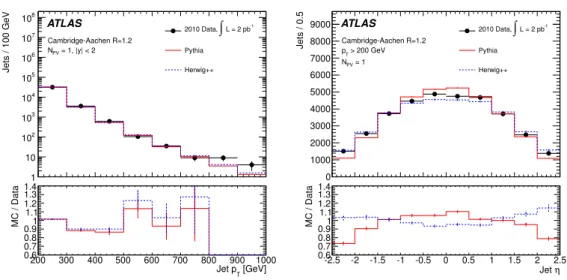
200 300 400 500 600 700 800 900 1000 Jets / 100 GeV 1 10 2 10 3 10 4 10 5 10 6 10 7 10 8 10 -1 L = 2 pb ∫ 2010 Data, Pythia Herwig++ Cambridge-Aachen R=1.2 = 1, |y| < 2 PV N ATLAS [GeV] T Jet p 200 300 400 500 600 700 800 900 1000 MC / Data 0.6 0.7 0.8 0.91 1.1 1.2 1.3 1.4 -2.5 -2 -1.5 -1 -0.5 0 0.5 1 1.5 2 2.5 Jets / 0.5 0 1000 2000 3000 4000 5000 6000 7000 8000 9000 -1 L = 2 pb ∫ 2010 Data, Pythia Herwig++ Cambridge-Aachen R=1.2 > 200 GeV T p = 1 PV N ATLAS η Jet -2.5 -2 -1.5 -1 -0.5 0 0.5 1 1.5 2 2.5 MC / Data 0.6 0.7 0.8 0.91 1.1 1.2 1.3 1.4Figure 1. pT (left) and η distribution (right) of Cambridge-Aachen R = 1.2 jets with pT > 200 GeV.
use the AMBT1 tune [28]. In some figures the Perugia2010 Pythia tune is used [37], which has been found to describe jet shapes more accurately at ATLAS [14]. Leading-order parton density functions are taken from the MRST2007 LO* set [38,39], unless stated otherwise. No pile-up was included in any of these samples.
The MC generated samples are passed through a full simulation [40] of the ATLAS de-tector and trigger, based on GEANT4 [41]. The Quark Gluon String Precompound (QGSP) model is used for the fragmentation of nuclei, and the Bertini cascade (BERT) model for the description of the interactions of the hadrons in the medium of the nucleus [42].
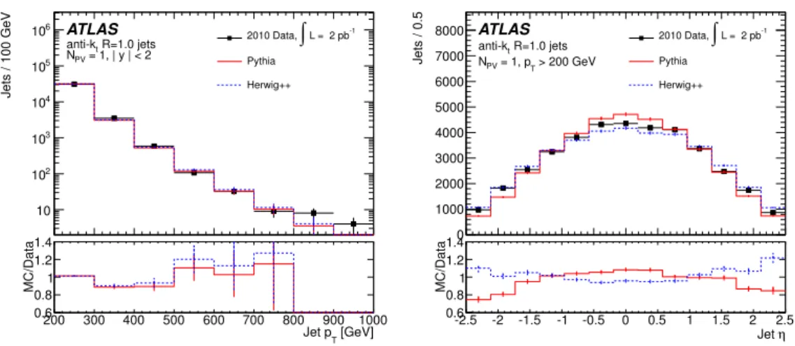
6 Detector-level distributions
Detector-level distributions for jet pT, η, mass,
√ d12,
√
d23, τ21 and τ32 are shown in
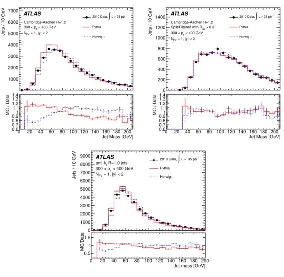
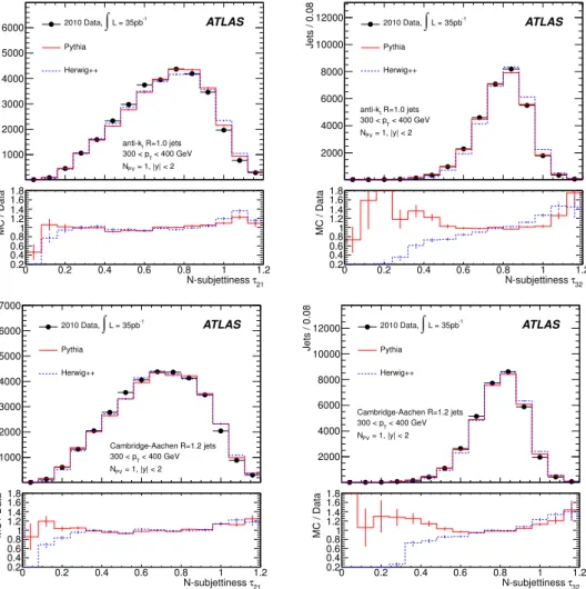
figures1–6. The statistical uncertainty represented in ratios is that from Monte Carlo and data added in quadrature. Representative distributions of the substructure variables are shown for the 300–400 GeV bin only. The Monte Carlo is normalised to the data separately in each plot. The properties of these jets are observed to be reasonably well modelled by leading-order parton-shower Monte Carlo. There are approximately four times fewer split and filtered jets (e.g. figure3) because many jets fail the splitting criteria described above.
7 Systematic uncertainties
The modelling of the calorimeter response is the biggest systematic uncertainty for this analysis. The key issue therefore is to validate the Monte Carlo-based jet calibration de-scribed in section 4. As the results here use jet algorithms with larger R-parameters, the ATLAS jet energy scale uncertainty [25] for anti-ktR = 0.4 and 0.6 jets cannot be applied.
JHEP05(2012)128
[GeV] T Jet p 200 300 400 500 600 700 800 900 1000 Jets / 100 GeV 10 2 10 3 10 4 10 5 10 6 10 ATLAS -1 L = 2 pb ∫ 2010 Data, Pythia Herwig++ R=1.0 jets t anti-k = 1, | y | < 2 PV N [GeV] T Jet p 200 300 400 500 600 700 800 900 1000 MC/Data 0.6 0.8 1 1.2 1.4 η Jet -2.5 -2 -1.5 -1 -0.5 0 0.5 1 1.5 2 2.5 Jets / 0.5 0 1000 2000 3000 4000 5000 6000 7000 8000 ATLAS -1 L = 2 pb ∫ 2010 Data, Pythia Herwig++ R=1.0 jets t anti-k > 200 GeV T = 1, p PV N η Jet -2.5 -2 -1.5 -1 -0.5 0 0.5 1 1.5 2 2.5 MC/Data 0.6 0.8 1 1.2 1.4Figure 2. pT(left) and η distribution (right) of anti-ktR = 1.0 jets with pT> 200 GeV.
200 300 400 500 600 700 800 900 1000 Jets / 100 GeV 1 10 2 10 3 10 4 10 5 10 6 10 7 10 8 10 -1 L = 2 pb ∫ 2010 Data, Pythia Herwig++ Cambridge-Aachen R=1.2 > 0.3 qq Split/Filtered with R = 1, |y| < 2 PV N ATLAS [GeV] T Jet p 200 300 400 500 600 700 800 900 1000 MC / Data 0.6 0.7 0.8 0.91 1.1 1.2 1.3 1.4 -2.5 -2 -1.5 -1 -0.5 0 0.5 1 1.5 2 2.5 Jets / 0.5 0 500 1000 1500 2000 2500 -1 L = 2 pb ∫ 2010 Data, Pythia Herwig++ Cambridge-Aachen R=1.2 > 0.3 qq Split/Filtered with R > 200 GeV T p = 1 PV N ATLAS η Jet -2.5 -2 -1.5 -1 -0.5 0 0.5 1 1.5 2 2.5 MC / Data 0.6 0.7 0.8 0.91 1.1 1.2 1.3 1.4
Figure 3. pT (left) and η distribution (right) of Cambridge-Aachen R = 1.2 jets after splitting and filtering with pT> 200 GeV.
The primary systematic uncertainties considered in the present study are those relating to scales and resolutions, such as jet pT scale (JES) and jet pT resolution (JER). For each
substructure variable, the scale and resolution of the variable itself are also considered, for example the jet mass scale (JMS) and jet mass resolution (JMR). The scale uncertainties are primarily constrained by in-situ validation using track-jets. The inner detector and calorimeter have largely uncorrelated systematic effects, therefore comparison of variables such as jet mass and energy between the two sub-detectors allows for some separation of physics and detector effects. This technique is limited to a precision of around 3-5% by systematic uncertainties arising from the inner-detector tracking efficiency and confidence in Monte Carlo modelling of the relative behaviour of the charged and neutral compo-nents of jets.
JHEP05(2012)128
0 20 40 60 80 100 120 140 160 180 200 Jets / 10 GeV 1000 2000 3000 4000 5000 6000 7000 -1 L = 35 pb ∫ 2010 Data, Pythia Herwig++ Cambridge-Aachen R=1.2 < 400 GeV T 300 < p = 1, |y| < 2 PV N ATLASJet Mass [GeV] 0 20 40 60 80 100 120 140 160 180 200 MC / Data 0.6 0.7 0.8 0.91 1.1 1.2 1.3 1.4 0 20 40 60 80 100 120 140 160 180 200 Jets / 10 GeV 0 200 400 600 800 1000 1200 1400 -1 L = 35 pb ∫ 2010 Data, Pythia Herwig++ Cambridge-Aachen R=1.2 > 0.3 qq Split/Filtered with R < 400 GeV T 300 < p = 1, |y| < 2 PV N ATLAS
Jet Mass [GeV] 0 20 40 60 80 100 120 140 160 180 200 MC / Data 0.6 0.7 0.8 0.91 1.1 1.2 1.3 1.4 [GeV] j m 0 20 40 60 80 100 120 140 160 180 200 Jets / 10 GeV 0 1000 2000 3000 4000 5000 6000 7000 8000 9000 ATLAS -1 L = 35 pb ∫ 2010 Data, Pythia Herwig++ R=1.0 jets t anti-k = 1, |y| < 2 PV N < 400 GeV T 300 < p
Jet mass [GeV] 0 20 40 60 80 100 120 140 160 180 200
MC/Data
0.5 1 1.5
Figure 4. Mass distributions for jets with |y| < 2.0 in the 300–400 GeV pT bin. Jets shown are Cambridge-Aachen (top left), Cambridge-Aachen after splitting and filtering (top right) and anti-kt(bottom).
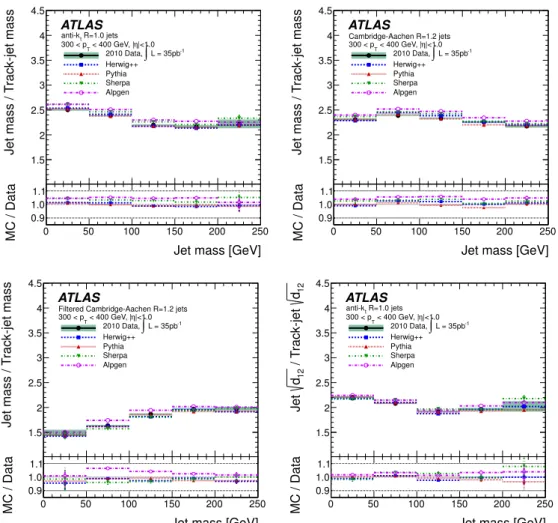
Jets composed from tracks are matched to calorimeter-jets if they are within δR < 0.3 of each other. The split and filtered calorimeter-jets are matched to Cambridge-Aachen R = 1.2 track-jets. Ratios are defined between track- and calorimeter-jets for each variable X (pT, mass, √ d12, √ d23, τ21, τ32): rX = Xcalorimeter−jet Xtrack−jet (7.1) Example distributions of some of the ratio variables are shown in figure 7. It can be seen that the ratios are in broad agreement between data and Monte Carlo. To quantify the level of agreement, double ratios are defined:
ρX = r X data rX MC , (7.2)
JHEP05(2012)128
[GeV] 12 d 0 10 20 30 40 50 60 70 80 90 100 Jets / 5 GeV 0 2000 4000 6000 8000 10000 ATLAS -1 L = 35 pb ∫ 2010 Data, Pythia Herwig++ R=1.0 jets t anti-k = 1, |y| < 2 PV N < 400 GeV T 300 < p [GeV] 12 d 0 10 20 30 40 50 60 70 80 90 100 MC/Data 0.5 1 1.5 [GeV] 23 d 0 5 10 15 20 25 30 35 40 Jets / 2 GeV 0 2000 4000 6000 8000 10000 ATLAS -1 L = 35 pb ∫ 2010 Data, Pythia Herwig++ R=1.0 jets t anti-k = 1, |y| < 2 PV N < 400 GeV T 300 < p [GeV] 23 d 0 5 10 15 20 25 30 35 40 MC/Data 0.5 1 1.5Figure 5. Distributions for √d12 (left) and √
d23 (right) of anti-ktR = 1.0 jets with |y| < 2.0 in the 300–400 GeV pT bin.
Jets / 0.08 1000 2000 3000 4000 5000 6000 2010 Data, ∫ L = 35pb-1 Pythia Herwig++ R=1.0 jets t anti-k < 400 GeV T 300 < p = 1, |y| < 2 PV N ATLAS 21 τ N-subjettiness 0 0.2 0.4 0.6 0.8 1 1.2 MC / Data 0.2 0.4 0.6 0.81 1.2 1.4 1.6 1.8 Jets / 0.08 2000 4000 6000 8000 10000 12000 2010 Data, ∫ L = 35pb-1 Pythia Herwig++ R=1.0 jets t anti-k < 400 GeV T 300 < p = 1, |y| < 2 PV N ATLAS 32 τ N-subjettiness 0 0.2 0.4 0.6 0.8 1 1.2 MC / Data 0.2 0.4 0.6 0.81 1.2 1.4 1.6 1.8 Jets / 0.08 1000 2000 3000 4000 5000 6000 7000 -1 L = 35pb ∫ 2010 Data, Pythia Herwig++ Cambridge-Aachen R=1.2 jets < 400 GeV T 300 < p = 1, |y| < 2 PV N ATLAS 21 τ N-subjettiness 0 0.2 0.4 0.6 0.8 1 1.2 MC / Data 0.2 0.4 0.6 0.81 1.2 1.4 1.6 1.8 Jets / 0.08 2000 4000 6000 8000 10000 12000 2010 Data, ∫ L = 35pb-1 Pythia Herwig++ Cambridge-Aachen R=1.2 jets < 400 GeV T 300 < p = 1, |y| < 2 PV N ATLAS 32 τ N-subjettiness 0 0.2 0.4 0.6 0.8 1 1.2 MC / Data 0.2 0.4 0.6 0.81 1.2 1.4 1.6 1.8
Figure 6. Distributions for τ21 (left) and τ32 (right) of jets with |y| < 2.0 in the 300–400 GeVpT bin for anti-kt(top) and Cambridge-Aachen jets (bottom).
JHEP05(2012)128
Je t m as s / T ra ck -je t m as s 1.5 2 2.5 3 3.5 4 4.5Jet mass [GeV]
0 50 100 150 200 250 MC / Data 0.9 1.0 1.1 ATLAS R=1.0 jets t anti-k |<1.0 η < 400 GeV, | T 300 < p -1 L = 35pb ∫ 2010 Data, Herwig++ Pythia Sherpa Alpgen Je t m as s / T ra ck -je t m as s 1.5 2 2.5 3 3.5 4 4.5
Jet mass [GeV]
0 50 100 150 200 250 MC / Data 0.9 1.0 1.1 ATLAS Cambridge-Aachen R=1.2 jets |<1.0 η < 400 GeV, | T 300 < p -1 L = 35pb ∫ 2010 Data, Herwig++ Pythia Sherpa Alpgen Je t m as s / T ra ck -je t m as s 1.5 2 2.5 3 3.5 4 4.5
Jet mass [GeV]
0 50 100 150 200 250 MC / Data 0.9 1.0 1.1 ATLAS
Filtered Cambridge-Aachen R=1.2 jets |<1.0 η < 400 GeV, | T 300 < p -1 L = 35pb ∫ 2010 Data, Herwig++ Pythia Sherpa Alpgen 12 d / Tr ac k-je t 12 d Jet 1.5 2 2.5 3 3.5 4 4.5
Jet mass [GeV]
0 50 100 150 200 250 MC / Data 0.9 1.0 1.1 ATLAS R=1.0 jets t anti-k |<1.0 η < 400 GeV, | T 300 < p -1 L = 35pb ∫ 2010 Data, Herwig++ Pythia Sherpa Alpgen
Figure 7. The ratio of a jet property determined by the calorimeter to that determined by tracks versus the calorimeter jet mass for jets with 300–400 GeV in pT. Shown are the data and a variety of Monte Carlo models. The bottom frame shows the ratio of the Monte Carlo models to data. The top left, top right and bottom left figures show the ratio for jet mass for three different jet algorithms. The bottom-right figure shows the ratios for√d12 in anti-ktjets.
where again, X can be pT, mass or any of the substructure variables. The distributions
of the variables Xcalorimeter−jet themselves are not necessarily expected to be correctly
modelled by Monte Carlo. However, if the simulation correctly models the effect of the detector on these variables, the double ratios ρX, are expected to be consistent with unity. Figure 7 also shows below each plot the corresponding double ratio. In order to account for possible uncertainties due to different fragmentation and hadronisation models, these double ratios are also calculated with a variety of Monte Carlo programs.
Final scale uncertainties are determined by adding in quadrature the estimated uncer-tainty on the inner-detector measurement with the deviation from unity observed in the double ratios. The resulting scale uncertainties on pT, mass and substructure variables are
sta-JHEP05(2012)128
tistical fluctuations when calculating the double ratio deviation. These scale uncertainties tend to dominate the systematic uncertainties on the final measurements.
As an additional cross-check, Monte Carlo-based tests are used to determine the depen-dence of the detector response on a number of different variables. These include samples produced with modified detector geometry, different GEANT hadronic physics models and different Monte Carlo generators. These tests indicate variations of a similar order of magnitude to those observed in the in-situ studies. The in-situ track-jet study is limited by inner-detector acceptance and only extends as far as |η| < 1.0, which corresponds to ' 75% of the jets in the measured distributions. However, the Monte Carlo-based tests also indicate no strong η-dependence from any of the different possible types of mismodelling examined. Based on this, the systematic uncertainty is applied to the entire sample.
In-situ tests of the JER [43] for anti-kt jets with R = 0.4 and 0.6 indicate that the
jet pT resolution predicted by simulation is in good agreement with that observed in the
data. Here, the resolution uncertainties are taken from the Monte Carlo tests described above only, primarily because the mass and substructure variable resolutions are difficult to validate in-situ with this dataset. From studying the variations in resolution created by varying the detector geometry, GEANT hadronic physics model and Monte Carlo generator, resolution uncertainties of around 20% are conservatively estimated, except for τ21and τ32
where they are around 10%.
8 Data correction
To compare the measurements directly to theoretical predictions the final distributions in this study are corrected for detector resolution and acceptance effects. The procedure here is a matrix-based unfolding technique called Iterative Dynamically Stabilised (IDS) unfolding [44,45].
In this procedure truth jets and reconstructed jets in Monte Carlo simulated events are matched using the criterion δR < 0.2, which leads to a match for > 99% of jets. Matched pairs of jets are used to construct a transfer matrix corresponding to the effect of the detector. A true jet can be matched with a reconstructed jet that fails the pT cut and
vice-versa. As such, the efficiency for matching a true jet to a reconstructed jet in the same pT bin is recorded as a function of the variable of interest. The reverse quantity is also
defined for reconstructed jets. The data are then scaled by the reconstructed matching efficiency, multiplied by the transfer matrix and finally divided by the truth matching efficiency. There is also an iterative optimisation step, where the rows of the matrix are scaled to match the corrected result. Pythia is used to provide the central value. Each pT bin is unfolded independently. The systematic uncertainty is assessed by repeating the
procedure using Sherpa samples.
9 Results
Using the analysis techniques outlined above, measured normalised cross-sections are shown in figures8–16. In ratio plots, the statistical uncertainty on Monte Carlo predictions does
JHEP05(2012)128
0 20 40 60 80 100 120 140 160 180 200 GeV 1 dm σ d σ 1 0 0.005 0.01 0.015 0.02 0.025 -1 L = 2 pb ∫ 2010 Data, Statistical Unc. Total Unc. Pythia Herwig++ Cambridge-Aachen R=1.2 < 300 GeV T 200 < p = 1, |y| < 2 PV N ATLASJet Mass [GeV]
0 20 40 60 80 100 120 140 160 180 200 MC / Data 0.2 0.4 0.6 0.81 1.2 1.4 1.6 1.8 MC / Data 0.2 0.4 0.6 0.81 1.2 1.4 1.6 1.8 0 20 40 60 80 100 120 140 160 180 200 GeV 1 dm σ d σ 1 0 0.002 0.004 0.006 0.008 0.01 0.012 0.014 0.016 0.018 2010 Data, ∫ L = 35 pb-1 Statistical Unc. Total Unc. Pythia Herwig++ Cambridge-Aachen R=1.2 < 400 GeV T 300 < p = 1, |y| < 2 PV N ATLAS
Jet Mass [GeV]
0 20 40 60 80 100 120 140 160 180 200 MC / Data 0.2 0.4 0.6 0.81 1.2 1.4 1.6 1.8 MC / Data 0.2 0.4 0.6 0.81 1.2 1.4 1.6 1.8 0 50 100 150 200 250 300 GeV 1 dm σ d σ 1 0 0.002 0.004 0.006 0.008 0.01 0.012 0.014 0.016 -1 L = 35 pb ∫ 2010 Data, Statistical Unc. Total Unc. Pythia Herwig++ Cambridge-Aachen R=1.2 < 500 GeV T 400 < p = 1, |y| < 2 PV N ATLAS
Jet Mass [GeV]
0 50 100 150 200 250 300 MC / Data 0.2 0.4 0.6 0.81 1.2 1.4 1.6 1.8 MC / Data 0.2 0.4 0.6 0.81 1.2 1.4 1.6 1.8 0 50 100 150 200 250 300 GeV 1 dm σ d σ 1 0 0.002 0.004 0.006 0.008 0.01 0.012 0.014 2010 Data, ∫ L = 35 pb-1 Statistical Unc. Total Unc. Pythia Herwig++ Cambridge-Aachen R=1.2 < 600 GeV T 500 < p = 1, |y| < 2 PV N ATLAS
Jet Mass [GeV]
0 50 100 150 200 250 300 MC / Data 0.2 0.4 0.6 0.81 1.2 1.4 1.6 1.8 MC / Data 0.2 0.4 0.6 0.81 1.2 1.4 1.6 1.8
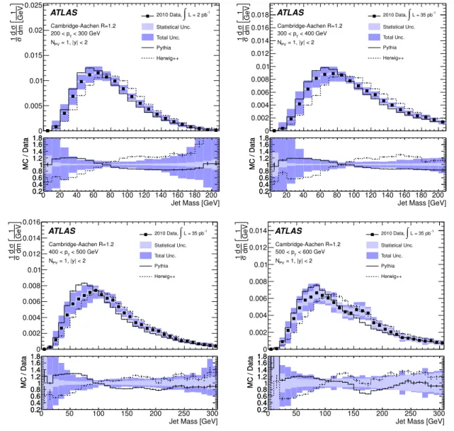
Figure 8. Normalised cross-sections as functions of mass of Cambridge-Aachen jets with R = 1.2 in four different pTbins.
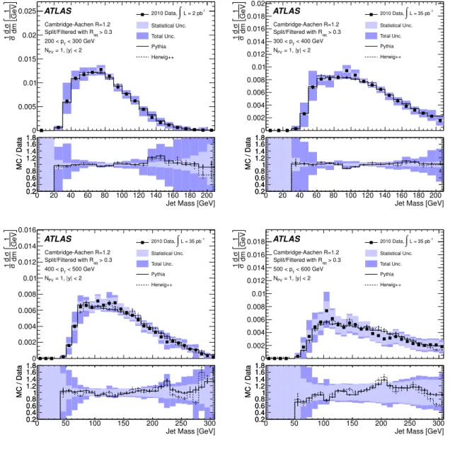
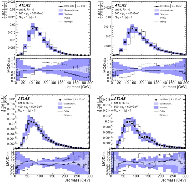
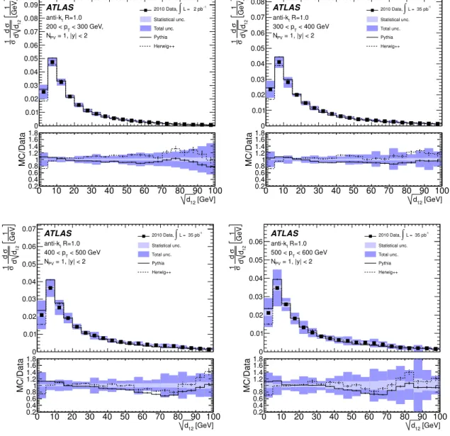
not include the data statistical uncertainty. Although in some cases the Monte Carlo predictions are not in agreement with the data, the shapes of the distributions are correctly reproduced. For jet mass the distributions produced by Pythia tend to be too soft, while those from Herwig++ are too hard. Notably, the Cambridge-Aachen jet mass after splitting and filtering, as shown in figure 9, is the only variable for which the Monte Carlo predictions are in agreement to within statistical uncertainties, both with each other and the data. The substructure variables exhibit generally better agreement with Monte Carlo predictions than mass, with all but a few bins correctly described by both Pythia and Herwig++. In the higher pTbins statistical fluctuations begin to limit the precision of the
measurements, but the level of agreement in all variables appears to remain approximately constant between pT bins.
JHEP05(2012)128
0 20 40 60 80 100 120 140 160 180 200 GeV 1 dm σ d σ 1 0 0.005 0.01 0.015 0.02 0.025 -1 L = 2 pb ∫ 2010 Data, Statistical Unc. Total Unc. Pythia Herwig++ Cambridge-Aachen R=1.2 > 0.3 qq Split/Filtered with R < 300 GeV T 200 < p = 1, |y| < 2 PV N ATLASJet Mass [GeV]
0 20 40 60 80 100 120 140 160 180 200 MC / Data 0.2 0.4 0.6 0.81 1.2 1.4 1.6 1.8 MC / Data 0.2 0.4 0.6 0.81 1.2 1.4 1.6 1.8 0 20 40 60 80 100 120 140 160 180 200 GeV 1 dm σ d σ 1 0 0.002 0.004 0.006 0.008 0.01 0.012 0.014 0.016 0.018 0.02 -1 L = 35 pb ∫ 2010 Data, Statistical Unc. Total Unc. Pythia Herwig++ Cambridge-Aachen R=1.2 > 0.3 qq Split/Filtered with R < 400 GeV T 300 < p = 1, |y| < 2 PV N ATLAS
Jet Mass [GeV]
0 20 40 60 80 100 120 140 160 180 200 MC / Data 0.2 0.4 0.6 0.81 1.2 1.4 1.6 1.8 MC / Data 0.2 0.4 0.6 0.81 1.2 1.4 1.6 1.8 0 50 100 150 200 250 300 GeV 1 dm σ d σ 1 0 0.002 0.004 0.006 0.008 0.01 0.012 0.014 0.016 -1 L = 35 pb ∫ 2010 Data, Statistical Unc. Total Unc. Pythia Herwig++ Cambridge-Aachen R=1.2 > 0.3 qq Split/Filtered with R < 500 GeV T 400 < p = 1, |y| < 2 PV N ATLAS
Jet Mass [GeV]
0 50 100 150 200 250 300 MC / Data 0.2 0.4 0.6 0.81 1.2 1.4 1.6 1.8 MC / Data 0.2 0.4 0.6 0.81 1.2 1.4 1.6 1.8 0 50 100 150 200 250 300 GeV 1 dm σ d σ 1 0 0.002 0.004 0.006 0.008 0.01 0.012 0.014 0.016 0.018 2010 Data, ∫ L = 35 pb-1 Statistical Unc. Total Unc. Pythia Herwig++ Cambridge-Aachen R=1.2 > 0.3 qq Split/Filtered with R < 600 GeV T 500 < p = 1, |y| < 2 PV N ATLAS
Jet Mass [GeV]
0 50 100 150 200 250 300 MC / Data 0.2 0.4 0.6 0.81 1.2 1.4 1.6 1.8 MC / Data 0.2 0.4 0.6 0.81 1.2 1.4 1.6 1.8
Figure 9. Normalised cross-sections as functions of mass of Cambridge-Aachen jets with R = 1.2 after splitting and filtering in four different pTbins.
The unfolding technique used introduces correlations between the bins. The statistical uncertainty in these results represents the diagonal element of the covariance matrix only; therefore, comparison to alternative predictions requires use of the full covariance matrices. These matrices are available, along with the full results presented here, in HepData [46]. In particular the structure at a jet mass of 150–180 GeV in the 500–600 GeV bin of figures8 and 10 is consistent with statistical fluctuations.
JHEP05(2012)128
0 20 40 60 80 100 120 140 160 180 200 GeV 1 d m σ d σ 1 0 0.005 0.01 0.015 0.02 0.025 0.03 0.035 ATLAS -1 L = 2 pb ∫ 2010 Data, Systematic unc. Total unc. Pythia Herwig++ = 1, |y| < 2 PV N R=1.0 t anti-k < 300 GeV, T 200 < pJet mass [GeV] 0 20 40 60 80 100 120 140 160 180 200 MC/Data 0.2 0.4 0.6 0.81 1.2 1.4 1.6 1.8 0 20 40 60 80 100 120 140 160 180 200 GeV 1 d m σ d σ 1 0 0.005 0.01 0.015 0.02 0.025 ATLAS -1 L = 35 pb ∫ 2010 Data, Systematic unc. Total unc. Pythia Herwig++ = 1, |y| < 2 PV N R=1.0 t anti-k < 400 GeV T 300 < p
Jet mass [GeV] 0 20 40 60 80 100 120 140 160 180 200 MC/Data 0.2 0.4 0.6 0.81 1.2 1.4 1.6 1.8 0 50 100 150 200 250 300 GeV 1 d m σ d σ 1 0 0.002 0.004 0.006 0.008 0.01 0.012 0.014 0.016 0.018 0.02 ATLAS -1 L = 35 pb ∫ 2010 Data, Statistical unc. Total unc. Pythia Herwig++ = 1, |y| < 2 PV N R=1.0 t anti-k < 500 GeV T 400 < p
Jet mass [GeV] 0 50 100 150 200 250 300 MC/Data 0.2 0.4 0.6 0.81 1.2 1.4 1.6 1.8 0 50 100 150 200 250 300 GeV 1 d m σ d σ 1 0 0.002 0.004 0.006 0.008 0.01 0.012 0.014 0.016 0.018 ATLAS -1 L = 35 pb ∫ 2010 Data, Statistical unc. Total unc. Pythia Herwig++ = 1, |y| < 2 PV N R=1.0 t anti-k < 600 GeV T 500 < p
Jet mass [GeV] 0 50 100 150 200 250 300 MC/Data 0.2 0.4 0.6 0.81 1.2 1.4 1.6 1.8
Figure 10. Normalised cross-sections as functions of mass of anti-kt jets with R = 1.0 in four different pTbins.
10 Mean mass with multiple proton-proton interactions
The results presented so far have been for events containing only one pp interaction; how-ever even in this early period of running, the data contain events with multiple simul-taneous pp interactions (pile-up) [47]. These additional collisions are uncorrelated with the hard-scattering process that typically triggers the event. They therefore present a background of soft, diffuse radiation that offsets the energy measurement of jets and will impact jet-shape and substructure measurements. It is essential that future studies involv-ing jet-substructure variables, such as those investigated here, be able to understand and correct for the effects of pile-up. Methods to mitigate these effects will be essential for jet multiplicity and energy scale measurements.
JHEP05(2012)128
0 10 20 30 40 50 60 70 80 90 100 GeV 1 12 d d σ d σ 1 0 0.01 0.02 0.03 0.04 0.05 0.06 0.07 0.08 0.09 ATLAS 2010 Data, ∫ L = 2 pb-1 Statistical unc. Total unc. Pythia Herwig++ = 1, |y| < 2 PV N R=1.0 t anti-k < 300 GeV, T 200 < p [GeV] 12 d 0 10 20 30 40 50 60 70 80 90 100 MC/Data 0.2 0.4 0.6 0.81 1.2 1.4 1.6 1.8 0 10 20 30 40 50 60 70 80 90 100 GeV 1 12 d d σ d σ 1 0 0.01 0.02 0.03 0.04 0.05 0.06 0.07 0.08 ATLAS -1 L = 35 pb ∫ 2010 Data, Statistical unc. Total unc. Pythia Herwig++ = 1, |y| < 2 PV N R=1.0 t anti-k < 400 GeV T 300 < p [GeV] 12 d 0 10 20 30 40 50 60 70 80 90 100 MC/Data 0.2 0.4 0.6 0.81 1.2 1.4 1.6 1.8 0 10 20 30 40 50 60 70 80 90 100 GeV 1 12 d d σ d σ 1 0 0.01 0.02 0.03 0.04 0.05 0.06 0.07 ATLAS -1 L = 35 pb ∫ 2010 Data, Statistical unc. Total unc. Pythia Herwig++ = 1, |y| < 2 PV N R=1.0 t anti-k < 500 GeV T 400 < p [GeV] 12 d 0 10 20 30 40 50 60 70 80 90 100 MC/Data 0.2 0.4 0.6 0.81 1.2 1.4 1.6 1.8 0 10 20 30 40 50 60 70 80 90 100 GeV 1 12 d d σ d σ 1 0 0.01 0.02 0.03 0.04 0.05 0.06 ATLAS -1 L = 35 pb ∫ 2010 Data, Statistical unc. Total unc. Pythia Herwig++ = 1, |y| < 2 PV N R=1.0 t anti-k < 600 GeV T 500 < p [GeV] 12 d 0 10 20 30 40 50 60 70 80 90 100 MC/Data 0.2 0.4 0.6 0.81 1.2 1.4 1.6 1.8Figure 11. Normalised cross-sections as functions of √d12 of anti-kt jets with R = 1.0 in four different pTbins.
Substructure observables are expected to be especially sensitive to pile-up [8]. This is true in particular for the invariant mass of large-size jets. Techniques such as the splitting and filtering procedure used in this study reduce the effective area of large jets and are therefore expected to reduce sensitivity to pile-up.
The sensitivity of mean jet mass to pile-up is tested in this dataset. The correlation of the mean jet mass of anti-kt jets with the number of reconstructed primary vertices is
presented in figure 17 (left). All jets with a pT of at least 300 GeV in the rapidity range
|y| < 2 are considered. The mean mass of jets in the absence of pile-up and the variation with pile-up activity show the expected dependence on the jet size. The mean mass in the
JHEP05(2012)128
0 5 10 15 20 25 30 35 40 GeV 1 23 d d σ d σ 1 0 0.02 0.04 0.06 0.08 0.1 0.12 0.14 0.16 0.18 0.2 0.22 0.24 ATLAS -1 L = 2 pb ∫ 2010 Data, Statistical unc. Total unc. Pythia Herwig++ = 1, |y| < 2 PV N R=1.0 t anti-k < 300 GeV, T 200 < p [GeV] 23 d 0 5 10 15 20 25 30 35 40 MC/Data 0.2 0.4 0.6 0.81 1.2 1.4 1.6 1.8 0 5 10 15 20 25 30 35 40 GeV 1 23 d d σ d σ 1 0 0.02 0.04 0.06 0.08 0.1 0.12 0.14 0.16 0.18 0.2 ATLAS -1 L = 35 pb ∫ 2010 Data, Statistical unc. Total unc. Pythia Herwig++ = 1, |y| < 2 PV N R=1.0 t anti-k < 400 GeV T 300 < p [GeV] 23 d 0 5 10 15 20 25 30 35 40 MC/Data 0.2 0.4 0.6 0.81 1.2 1.4 1.6 1.8 0 5 10 15 20 25 30 35 40 GeV 1 23 d d σ d σ 1 0 0.02 0.04 0.06 0.08 0.1 0.12 0.14 0.16 0.18 ATLAS -1 L = 35 pb ∫ 2010 Data, Statistical unc. Total unc. Pythia Herwig++ = 1, |y| < 2 PV N R=1.0 t anti-k < 500 GeV T 400 < p [GeV] 23 d 0 5 10 15 20 25 30 35 40 MC/Data 0.2 0.4 0.6 0.81 1.2 1.4 1.6 1.8 0 5 10 15 20 25 30 35 40 GeV 1 23 d d σ d σ 1 0 0.02 0.04 0.06 0.08 0.1 0.12 0.14 0.16 0.18 ATLAS -1 L = 35 pb ∫ 2010 Data, Statistical unc. Total unc. Pythia Herwig++ = 1, |y| < 2 PV N R=1.0 t anti-k < 600 GeV T 500 < p [GeV] 23 d 0 5 10 15 20 25 30 35 40 MC/Data 0.2 0.4 0.6 0.81 1.2 1.4 1.6 1.8Figure 12. Normalised cross-sections as functions of √d23 of anti-kt jets with R = 1.0 in four different pTbins.
NPV = 1 bin increases linearly with R. The ratios of the fitted slopes sR are found to be:
s1.0/s0.6= 4.3 ± 0.5 ((1.0/0.6)3= 4.6), (10.1)
s1.0/s0.4= 13 ± 3 ((1.0/0.4)3= 15.6), (10.2)
s0.6/s0.4= 3.0 ± 0.8 ((0.6/0.4)3= 3.4), (10.3)
in good agreement with the ratio of the third power of the jet R-parameter. This is in agreement with predictions of scaling of the mean mass [48,49]. This behaviour can also be qualitatively explained by two factors. Firstly the jet area in the y − φ plane grows roughly as R2. Moreover, the contribution of these particles to the jet mass scales with the distance between them approximately as R/2, giving another power of R.
JHEP05(2012)128
0 0.2 0.4 0.6 0.8 1 1.2 21 τ d σ d σ 1 0 0.5 1 1.5 2 2.5 3 2010 Data, ∫ L = 2pb-1 Statistical Unc. Total Unc. Pythia Herwig++ Cambridge-Aachen R=1.2 jets < 300 GeV T 200 < p = 1, |y| < 2 PV N ATLAS 21 τ N-subjettiness 0 0.2 0.4 0.6 0.8 1 1.2 MC / Data 0.2 0.4 0.6 0.81 1.2 1.4 1.6 1.8 0 0.2 0.4 0.6 0.8 1 1.2 21 τ d σ d σ 1 0 0.5 1 1.5 2 2.5 -1 L = 35pb ∫ 2010 Data, Statistical Unc. Total Unc. Pythia Herwig++ Cambridge-Aachen R=1.2 jets < 400 GeV T 300 < p = 1, |y| < 2 PV N ATLAS 21 τ N-subjettiness 0 0.2 0.4 0.6 0.8 1 1.2 MC / Data 0.2 0.4 0.6 0.81 1.2 1.4 1.6 1.8 0 0.2 0.4 0.6 0.8 1 1.2 21 τ d σ d σ 1 0 0.5 1 1.5 2 2.5 3 -1 L = 35pb ∫ 2010 Data, Statistical Unc. Total Unc. Pythia Herwig++ Cambridge-Aachen R=1.2 jets < 500 GeV T 400 < p = 1, |y| < 2 PV N ATLAS 21 τ N-subjettiness 0 0.2 0.4 0.6 0.8 1 1.2 MC / Data 0.2 0.4 0.6 0.81 1.2 1.4 1.6 1.8 0 0.2 0.4 0.6 0.8 1 1.2 21 τ d σ d 1 σ 0 0.5 1 1.5 2 2.5 3 -1 L = 35pb ∫ 2010 Data, Statistical Unc. Total Unc. Pythia Herwig++ Cambridge-Aachen R=1.2 jets < 600 GeV T 500 < p = 1, |y| < 2 PV N ATLAS 21 τ N-subjettiness 0 0.2 0.4 0.6 0.8 1 1.2 MC / Data 0.2 0.4 0.6 0.81 1.2 1.4 1.6 1.8Figure 13. Normalised cross-sections as functions of τ21 of Cambridge-Aachen jets with R = 1.2 in four different pTbins.
Figure 17 (right) shows the dependence on NPV of the mean jet mass before and
after the splitting and filtering procedure for Cambridge-Aachen jets. Since the angular requirement Rjj > 0.3 is imposed, the splitting steps of this procedure naturally select
more massive jets. Since the splitting procedure selects a kinematically biased subset of jets, a third line shows the mean mass prior to filtering of jets that pass the splitting. The filtering step significantly reduces the impact of pile-up on mean jet mass. In fact, the slope of the straight line fitted to the filtered jet data points is statistically consistent with zero. Altogether, this demonstrates that the pile-up dependence of mean jet mass in real LHC conditions matches expectations. Additionally, jet substructure techniques that re-duce the area of jets are promising for suppressing the effects of pile-up.
JHEP05(2012)128
0 0.2 0.4 0.6 0.8 1 1.2 32 τ d σ d σ 1 0 1 2 3 4 5 2010 Data, ∫ L = 2pb-1 Statistical Unc. Total Unc. Pythia Herwig++ Cambridge-Aachen R=1.2 jets < 300 GeV T 200 < p = 1, |y| < 2 PV N ATLAS 32 τ N-subjettiness 0 0.2 0.4 0.6 0.8 1 1.2 MC / Data 0.2 0.4 0.6 0.81 1.2 1.4 1.6 1.8 0 0.2 0.4 0.6 0.8 1 1.2 32 τ d σ d σ 1 0 1 2 3 4 5 2010 Data, ∫ L = 35pb-1 Statistical Unc. Total Unc. Pythia Herwig++ Cambridge-Aachen R=1.2 jets < 400 GeV T 300 < p = 1, |y| < 2 PV N ATLAS 32 τ N-subjettiness 0 0.2 0.4 0.6 0.8 1 1.2 MC / Data 0.2 0.4 0.6 0.81 1.2 1.4 1.6 1.8 0 0.2 0.4 0.6 0.8 1 1.2 32 τ d σ d σ 1 0 1 2 3 4 5 -1 L = 35pb ∫ 2010 Data, Statistical Unc. Total Unc. Pythia Herwig++ Cambridge-Aachen R=1.2 jets < 500 GeV T 400 < p = 1, |y| < 2 PV N ATLAS 32 τ N-subjettiness 0 0.2 0.4 0.6 0.8 1 1.2 MC / Data 0.2 0.4 0.6 0.81 1.2 1.4 1.6 1.8 0 0.2 0.4 0.6 0.8 1 1.2 32 τ d σ d 1 σ 0 1 2 3 4 -1 L = 35pb ∫ 2010 Data, Statistical Unc. Total Unc. Pythia Herwig++ Cambridge-Aachen R=1.2 jets < 600 GeV T 500 < p = 1, |y| < 2 PV N ATLAS 32 τ N-subjettiness 0 0.2 0.4 0.6 0.8 1 1.2 MC / Data 0.2 0.4 0.6 0.81 1.2 1.4 1.6 1.8Figure 14. Normalised cross-sections as functions of τ32 of Cambridge-Aachen jets with R = 1.2 in four different pTbins.
11 Conclusions
Jet mass and several jet substructure variables have been measured. This is the first particle-level measurement of these variables at the LHC and in many cases the first at any experiment. There is broad agreement between data and leading-order parton-shower Monte Carlo predictions from Pythia and Herwig++, although there is some scope to improve this. Jet mass has generally been found to exhibit the largest disagreements with Monte Carlo simulations. However, in contrast to this, the masses of jets after the Cambridge-Aachen splitting and filtering procedure display good agreement both with and
JHEP05(2012)128
0 0.2 0.4 0.6 0.8 1 1.2 21 τ d σ d σ 1 0 0.5 1 1.5 2 2.5 -1 L = 2pb ∫ 2010 Data, Statistical Unc. Total Unc. Pythia Herwig++ R=1.0 jets t anti-k < 300 GeV T 200 < p = 1, |y| < 2 PV N ATLAS 21 τ N-subjettiness 0 0.2 0.4 0.6 0.8 1 1.2 MC / Data 0.2 0.4 0.6 0.81 1.2 1.4 1.6 1.8 0 0.2 0.4 0.6 0.8 1 1.2 21 τ d σ d σ 1 0 0.5 1 1.5 2 2.5 -1 L = 35pb ∫ 2010 Data, Statistical Unc. Total Unc. Pythia Herwig++ R=1.0 jets t anti-k < 400 GeV T 300 < p = 1, |y| < 2 PV N ATLAS 21 τ N-subjettiness 0 0.2 0.4 0.6 0.8 1 1.2 MC / Data 0.2 0.4 0.6 0.81 1.2 1.4 1.6 1.8 0 0.2 0.4 0.6 0.8 1 1.2 21 τ d σ d σ 1 0 0.5 1 1.5 2 2.5 -1 L = 35pb ∫ 2010 Data, Statistical Unc. Total Unc. Pythia Herwig++ R=1.0 jets t anti-k < 500 GeV T 400 < p = 1, |y| < 2 PV N ATLAS 21 τ N-subjettiness 0 0.2 0.4 0.6 0.8 1 1.2 MC / Data 0.2 0.4 0.6 0.81 1.2 1.4 1.6 1.8 0 0.2 0.4 0.6 0.8 1 1.2 21 τ d σ d 1 σ 0 0.5 1 1.5 2 2.5 -1 L = 35pb ∫ 2010 Data, Statistical Unc. Total Unc. Pythia Herwig++ R=1.0 jets t anti-k < 600 GeV T 500 < p = 1, |y| < 2 PV N ATLAS 21 τ N-subjettiness 0 0.2 0.4 0.6 0.8 1 1.2 MC / Data 0.2 0.4 0.6 0.81 1.2 1.4 1.6 1.8Figure 15. Normalised cross-sections as functions of τ21 of anti-kt jets with R = 1.0 in four different pTbins.
between Monte Carlo simulations. The substructure variables √d12,
√
d23, τ21 and τ32
are all reasonably well reproduced by Monte Carlo predictions. Additionally, the effects of pile-up on mean jet mass have been found to match phenomenological expectations for R-parameter dependence. Splitting and filtering has also been found to reduce the impact of pile-up significantly.
Generally these results show that jet mass and substructure quantities can be success-fully reproduced by leading-order parton-shower Monte Carlo. This result bodes well for future analyses aiming to make use of jet substructure techniques.
JHEP05(2012)128
0 0.2 0.4 0.6 0.8 1 1.2 32 τ d σ d 1 σ 0 1 2 3 4 5 6 -1 L = 2pb ∫ 2010 Data, Statistical Unc. Total Unc. Pythia Herwig++ R=1.0 jets t anti-k < 300 GeV T 200 < p = 1, |y| < 2 PV N ATLAS 32 τ N-subjettiness 0 0.2 0.4 0.6 0.8 1 1.2 MC / Data 0.2 0.4 0.6 0.81 1.2 1.4 1.6 1.8 0 0.2 0.4 0.6 0.8 1 1.2 32 τ d σ d σ 1 0 1 2 3 4 5 2010 Data, ∫ L = 35pb-1 Statistical Unc. Total Unc. Pythia Herwig++ R=1.0 jets t anti-k < 400 GeV T 300 < p = 1, |y| < 2 PV N ATLAS 32 τ N-subjettiness 0 0.2 0.4 0.6 0.8 1 1.2 MC / Data 0.2 0.4 0.6 0.81 1.2 1.4 1.6 1.8 0 0.2 0.4 0.6 0.8 1 1.2 32 τ d σ d σ 1 0 1 2 3 4 5 L = 35pb-1 ∫ 2010 Data, Statistical Unc. Total Unc. Pythia Herwig++ R=1.0 jets t anti-k < 500 GeV T 400 < p = 1, |y| < 2 PV N ATLAS 32 τ N-subjettiness 0 0.2 0.4 0.6 0.8 1 1.2 MC / Data 0.2 0.4 0.6 0.81 1.2 1.4 1.6 1.8 0 0.2 0.4 0.6 0.8 1 1.2 32 τ d σ d σ 1 0 1 2 3 4 5 L = 35pb-1 ∫ 2010 Data, Statistical Unc. Total Unc. Pythia Herwig++ R=1.0 jets t anti-k < 600 GeV T 500 < p = 1, |y| < 2 PV N ATLAS 32 τ N-subjettiness 0 0.2 0.4 0.6 0.8 1 1.2 MC / Data 0.2 0.4 0.6 0.81 1.2 1.4 1.6 1.8Figure 16. Normalised cross-sections as functions of τ32 of anti-kt jets with R = 1.0 in four different pTbins.
Acknowledgments
We thank CERN for the very successful operation of the LHC, as well as the support staff from our institutions without whom ATLAS could not be operated efficiently.
We acknowledge the support of ANPCyT, Argentina; YerPhI, Armenia; ARC, Aus-tralia; BMWF, Austria; ANAS, Azerbaijan; SSTC, Belarus; CNPq and FAPESP, Brazil; NSERC, NRC and CFI, Canada; CERN; CONICYT, Chile; CAS, MOST and NSFC, China; COLCIENCIAS, Colombia; MSMT CR, MPO CR and VSC CR, Czech Repub-lic; DNRF, DNSRC and Lundbeck Foundation, Denmark; ARTEMIS and ERC, European Union; IN2P3-CNRS, CEA-DSM/IRFU, France; GNAS, Georgia; BMBF, DFG, HGF,
JHEP05(2012)128
pv
N
1 2 3 4 5 6
Mean Jet Mass [GeV] / 1 PV
0 20 40 60 80 100 120 140 160 ATLAS > 300 GeV, |y| < 2 T jets, p t anti-k 0.1 ± = 3.0 PV R=1.0: d m / d N 0.1 ± = 0.7 PV R=0.6: d m / d N 0.1 ± = 0.2 PV R=0.4: d m / d N -1 L = 35 pb
∫
PV N 1 2 3 4 5 6 7 8 9Mean Jet Mass [GeV] / 1 PV
80 100 120 140 160 180 200 220 240 260 Before Splitting/Filtering After Splitting/Filtering After Splitting Only
Cambridge-Aachen R=1.2 jets > 0.3 qq Split/Filtered with R > 300 GeV, |y| < 2 T p 0.3 GeV ± = 2.9 PV dNdm 0.1 GeV ± = 4.2 PV dNdm 0.2 GeV ± = 0.1 PV dNdm ATLAS -1 L = 35 pb
∫
Figure 17. The mean mass for jets with pT > 300 GeV as a function of the number of primary vertices identified in the event. Comparisons show the effect for anti-kt jets with different R-parameters (left) and Cambridge-Aachen R = 1.2 jets with and without splitting and filtering procedure (right). Each set of points is fitted with a straight line.
MPG and AvH Foundation, Germany; GSRT, Greece; ISF, MINERVA, GIF, DIP and Benoziyo Center, Israel; INFN, Italy; MEXT and JSPS, Japan; CNRST, Morocco; FOM and NWO, Netherlands; RCN, Norway; MNiSW, Poland; GRICES and FCT, Portugal; MERYS (MECTS), Romania; MES of Russia and ROSATOM, Russian Federation; JINR; MSTD, Serbia; MSSR, Slovakia; ARRS and MVZT, Slovenia; DST/NRF, South Africa; MICINN, Spain; SRC and Wallenberg Foundation, Sweden; SER, SNSF and Cantons of Bern and Geneva, Switzerland; NSC, Taiwan; TAEK, Turkey; STFC, the Royal Society and Leverhulme Trust, United Kingdom; DOE and NSF, United States of America.
The crucial computing support from all WLCG partners is acknowledged gratefully, in particular from CERN and the ATLAS Tier-1 facilities at TRIUMF (Canada), NDGF (Denmark, Norway, Sweden), CC-IN2P3 (France), KIT/GridKA (Germany), INFN-CNAF (Italy), NL-T1 (Netherlands), PIC (Spain), ASGC (Taiwan), RAL (U.K.) and BNL (U.S.A.) and in the Tier-2 facilities worldwide.
Open Access. This article is distributed under the terms of the Creative Commons
Attribution License which permits any use, distribution and reproduction in any medium, provided the original author(s) and source are credited.
References
[1] S. Catani, Y.L. Dokshitzer, M. Seymour and B. Webber, Longitudinally invariant Kt clustering algorithms for hadron hadron collisions,Nucl. Phys. B 406 (1993) 187[INSPIRE]. [2] S.D. Ellis and D.E. Soper, Successive combination jet algorithm for hadron collisions,Phys.
JHEP05(2012)128
[3] Y.L. Dokshitzer, G. Leder, S. Moretti and B. Webber, Better jet clustering algorithms,JHEP 08 (1997) 001[hep-ph/9707323] [INSPIRE].
[4] M. Wobisch and T. Wengler, Hadronization corrections to jet cross-sections in deep inelastic scattering, Tecnical Report PITHA-99-16 (1999) [hep-ph/9907280] [INSPIRE].
[5] M. Cacciari, G.P. Salam and G. Soyez, The anti-kt jet clustering algorithm,JHEP 04 (2008)
063[arXiv:0802.1189] [INSPIRE].
[6] G.P. Salam and G. Soyez, A Practical Seedless Infrared-Safe Cone jet algorithm,JHEP 05 (2007) 086[arXiv:0704.0292] [INSPIRE].
[7] G.C. Blazey et al., Run II jet physics, Report FERMILAB-CONF-00-092-E (2000). [8] A. Abdesselam et al., Boosted objects: a probe of beyond the Standard Model physics,Eur.
Phys. J. C 71 (2011) 1661[arXiv:1012.5412] [INSPIRE].
[9] CDF collaboration, T. Aaltonen et al., Study of Substructure of High Transverse Momentum Jets Produced in Proton-Antiproton Collisions at√s = 1.96 TeV, Phys. Rev. D 85 (2012) 091101 [arXiv:1106.5952] [INSPIRE].
[10] ZEUS collaboration, S. Chekanov et al., Subjet distributions in deep inelastic scattering at HERA,Eur. Phys. J. C 63 (2009) 527[arXiv:0812.2864] [INSPIRE].
[11] CDF collaboration, D. Acosta et al., Study of jet shapes in inclusive jet production in p¯p collisions at√s = 1.96 TeV,Phys. Rev. D 71 (2005) 112002[hep-ex/0505013] [INSPIRE]. [12] ZEUS collaboration, S. Chekanov et al., Substructure dependence of jet cross sections at
HERA and determination of αs,Nucl. Phys. B 700 (2004) 3[hep-ex/0405065] [INSPIRE]. [13] ZEUS collaboration, S. Chekanov et al., Measurement of subjet multiplicities in neutral
current deep inelastic scattering at HERA and determination of αs, Phys. Lett. B 558
(2003) 41[hep-ex/0212030] [INSPIRE].
[14] ATLAS collaboration, G. Aad et al., Study of Jet Shapes in Inclusive Jet Production in pp Collisions at√s = 7 TeV using the ATLAS Detector, Phys. Rev. D 83 (2011) 052003 [arXiv:1101.0070] [INSPIRE].
[15] J. Butterworth, B. Cox and J.R. Forshaw, W W scattering at the CERN LHC,Phys. Rev. D 65 (2002) 096014[hep-ph/0201098] [INSPIRE].
[16] J. Thaler and K. Van Tilburg, Identifying boosted objects with N-subjettiness,JHEP 03 (2011) 015[arXiv:1011.2268] [INSPIRE].
[17] J.M. Butterworth, A.R. Davison, M. Rubin and G.P. Salam, Jet substructure as a new Higgs search channel at the LHC,Phys. Rev. Lett. 100 (2008) 242001[arXiv:0802.2470]
[INSPIRE].
[18] M. Cacciari and G.P. Salam, Dispelling the N3 myth for the k
t jet-finder,Phys. Lett. B 641
(2006) 57[hep-ph/0512210] [INSPIRE].
[19] ATLAS collaboration, ATLAS Sensitivity to the Standard Model Higgs in the HW and HZ Channels at High Transverse Momenta,ATL-PHYS-PUB-2009-088(2009).
[20] J. Thaler and K. Van Tilburg, Maximizing boosted top identification by minimizing N-subjettiness,JHEP 02 (2012) 093[arXiv:1108.2701] [INSPIRE].
[21] ATLAS collaboration, The ATLAS experiment at the CERN large Hadron Collider,2008 JINST 3 S08003.
JHEP05(2012)128
[22] ATLAS collaboration, G. Aad et al., Performance of the ATLAS Trigger System in 2010, Eur. Phys. J. C 72 (2012) 1849 [arXiv:1110.1530] [INSPIRE].
[23] ATLAS collaboration, G. Aad et al., Luminosity determination in pp collisions at√ s = 7 TeV using the ATLAS detector at the LHC, Eur. Phys. J. C 71 (2011) 1630 [arXiv:1101.2185] [INSPIRE].
[24] ATLAS collaboration, Updated luminosity determination in pp collisions at √s = 7 TeV using the ATLAS Detector,ATLAS-CONF-2011-011(2011).
[25] ATLAS collaboration, G. Aad et al., Jet energy measurement with the ATLAS detector in proton-proton collisions at√s = 7 TeV,arXiv:1112.6426[INSPIRE].
[26] ATLAS collaboration, Calorimeter clustering algorithms: description and performance,
ATL-LARG-PUB-2008-002(2008).
[27] T. Sj¨ostrand, S. Mrenna and P.Z. Skands, PYTHIA 6.4 physics and manual,JHEP 05 (2006) 026[hep-ph/0603175] [INSPIRE].
[28] ATLAS collaboration, G. Aad et al., Charged-particle multiplicities in pp interactions measured with the ATLAS detector at the LHC, New J. Phys. 13 (2011) 053033 [arXiv:1012.5104] [INSPIRE].
[29] M. Bahr et al., HERWIG++ physics and manual, Eur. Phys. J. C 58 (2008) 639
[arXiv:0803.0883] [INSPIRE].
[30] M.L. Mangano, M. Moretti, F. Piccinini, R. Pittau and A.D. Polosa, ALPGEN, a generator for hard multiparton processes in hadronic collisions,JHEP 07 (2003) 001[hep-ph/0206293] [INSPIRE].
[31] T. Gleisberg et al., Event generation with SHERPA 1.1,JHEP 02 (2009) 007
[arXiv:0811.4622] [INSPIRE].
[32] B. Andersson, G. Gustafson, G. Ingelman and T. Sj¨ostrand, Parton fragmentation and string dynamics,Phys. Rept. 97 (1983) 31[INSPIRE].
[33] B. Webber, A QCD model for jet fragmentation including soft gluon interference,Nucl. Phys. B 238 (1984) 492[INSPIRE].
[34] G. Corcella et al., HERWIG 6.5 release note,hep-ph/0210213[INSPIRE].
[35] G. Corcella et al., HERWIG 6: An event generator for hadron emission reactions with interfering gluons (including supersymmetric processes),JHEP 01 (2001) 010
[hep-ph/0011363] [INSPIRE].
[36] J. Butterworth, J.R. Forshaw and M. Seymour, Multiparton interactions in photoproduction at HERA,Z. Phys. C 72 (1996) 637[hep-ph/9601371] [INSPIRE].
[37] P.Z. Skands, Tuning Monte Carlo Generators: The Perugia Tunes,Phys. Rev. D 82 (2010) 074018[arXiv:1005.3457] [INSPIRE].
[38] A. Martin, W. Stirling, R. Thorne and G. Watt, Parton distributions for the LHC, Eur. Phys. J. C 63 (2009) 189[arXiv:0901.0002] [INSPIRE].
[39] A. Sherstnev and R. Thorne, Parton distributions for LO generators,Eur. Phys. J. C 55 (2008) 553[arXiv:0711.2473] [INSPIRE].
[40] ATLAS collaboration, G. Aad et al., The ATLAS simulation infrastructure,Eur. Phys. J. C 70 (2010) 823[arXiv:1005.4568] [INSPIRE].
JHEP05(2012)128
[41] GEANT4 collaboration, S. Agostinelli et al., GEANT4: A Simulation toolkit,Nucl. Instrum. Meth. A 506 (2003) 250[INSPIRE].
[42] A. Ribon et al., Status of GEANT4 hadronic physics for the simulation of LHC experiments at the start of LHC physics program,CERN-LCGAPP 2010-02(2010).
[43] ATLAS collaboration, Jet energy resolution and selection efficiency relative to track jets from in-situ techniques with the ATLAS Detector Using Proton-Proton Collisions at a Center of Mass Energy sqrts = 7 TeV,ATLAS-CONF-2010-054(2010).
[44] B. Malaescu, An Iterative, Dynamically Stabilized(IDS) Method of Data Unfolding,
arXiv:1106.3107[INSPIRE].
[45] B. Malaescu, An iterative, dynamically stabilized method of data unfolding,
arXiv:0907.3791[INSPIRE].
[46] ATLAS collaboration, HepData relating to this paper,
http://hepdata.cedar.ac.uk/view/red4953(2012).
[47] ATLAS collaboration, In-situ jet energy scale and jet shape corrections for multiple interactions in the first ATLAS data at the LHC,ATLAS-CONF-2011-030(2011). [48] M. Dasgupta, L. Magnea and G.P. Salam, Non-perturbative QCD effects in jets at hadron
colliders,JHEP 02 (2008) 055[arXiv:0712.3014] [INSPIRE].
[49] A. Altheimer et al., Jet Substructure at the Tevatron and LHC: New results, new tools, new benchmarks, proceedings of the BOOST 2011 conference, Princeton U.S.A. (2011)
[arXiv:1201.0008] [INSPIRE].
The ATLAS collaboration
G. Aad48, B. Abbott110, J. Abdallah11, S. Abdel Khalek114, A.A. Abdelalim49, A. Abdesselam117, O. Abdinov10, B. Abi111, M. Abolins87, O.S. AbouZeid157,
H. Abramowicz152, H. Abreu114, E. Acerbi88a,88b, B.S. Acharya163a,163b, L. Adamczyk37, D.L. Adams24, T.N. Addy56, J. Adelman174, M. Aderholz98, S. Adomeit97, P. Adragna74, T. Adye128, S. Aefsky22, J.A. Aguilar-Saavedra123b,a, M. Aharrouche80, S.P. Ahlen21, F. Ahles48, A. Ahmad147, M. Ahsan40, G. Aielli132a,132b, T. Akdogan18a,
T.P.A. ˚Akesson78, G. Akimoto154, A.V. Akimov93, A. Akiyama66, M.S. Alam1, M.A. Alam75, J. Albert168, S. Albrand55, M. Aleksa29, I.N. Aleksandrov64,
F. Alessandria88a, C. Alexa25a, G. Alexander152, G. Alexandre49, T. Alexopoulos9,
M. Alhroob20, M. Aliev15, G. Alimonti88a, J. Alison119, M. Aliyev10, B.M.M. Allbrooke17, P.P. Allport72, S.E. Allwood-Spiers53, J. Almond81, A. Aloisio101a,101b, R. Alon170,
A. Alonso78, B. Alvarez Gonzalez87, M.G. Alviggi101a,101b, K. Amako65, P. Amaral29, C. Amelung22, V.V. Ammosov127, A. Amorim123a,b, G. Amor´os166, N. Amram152, C. Anastopoulos29, L.S. Ancu16, N. Andari114, T. Andeen34, C.F. Anders20,
G. Anders58a, K.J. Anderson30, A. Andreazza88a,88b, V. Andrei58a, M-L. Andrieux55, X.S. Anduaga69, A. Angerami34, F. Anghinolfi29, A. Anisenkov106, N. Anjos123a, A. Annovi47, A. Antonaki8, M. Antonelli47, A. Antonov95, J. Antos143b, F. Anulli131a, S. Aoun82, L. Aperio Bella4, R. Apolle117,c, G. Arabidze87, I. Aracena142, Y. Arai65, A.T.H. Arce44, S. Arfaoui147, J-F. Arguin14, E. Arik18a,∗, M. Arik18a, A.J. Armbruster86,
JHEP05(2012)128
O. Arnaez80, V. Arnal79, C. Arnault114, A. Artamonov94, G. Artoni131a,131b,
D. Arutinov20, S. Asai154, R. Asfandiyarov171, S. Ask27, B. ˚Asman145a,145b, L. Asquith5, K. Assamagan24, A. Astbury168, A. Astvatsatourov52, B. Aubert4, E. Auge114,
K. Augsten126, M. Aurousseau144a, G. Avolio162, R. Avramidou9, D. Axen167, C. Ay54,
G. Azuelos92,d, Y. Azuma154, M.A. Baak29, G. Baccaglioni88a, C. Bacci133a,133b,
A.M. Bach14, H. Bachacou135, K. Bachas29, M. Backes49, M. Backhaus20, E. Badescu25a, P. Bagnaia131a,131b, S. Bahinipati2, Y. Bai32a, D.C. Bailey157, T. Bain157, J.T. Baines128, O.K. Baker174, M.D. Baker24, S. Baker76, E. Banas38, P. Banerjee92, Sw. Banerjee171, D. Banfi29, A. Bangert149, V. Bansal168, H.S. Bansil17, L. Barak170, S.P. Baranov93, A. Barashkou64, A. Barbaro Galtieri14, T. Barber48, E.L. Barberio85, D. Barberis50a,50b, M. Barbero20, D.Y. Bardin64, T. Barillari98, M. Barisonzi173, T. Barklow142, N. Barlow27, B.M. Barnett128, R.M. Barnett14, A. Baroncelli133a, G. Barone49, A.J. Barr117,
F. Barreiro79, J. Barreiro Guimar˜aes da Costa57, P. Barrillon114, R. Bartoldus142,
A.E. Barton70, V. Bartsch148, R.L. Bates53, L. Batkova143a, J.R. Batley27, A. Battaglia16, M. Battistin29, F. Bauer135, H.S. Bawa142,e, S. Beale97, T. Beau77, P.H. Beauchemin160, R. Beccherle50a, P. Bechtle20, H.P. Beck16, S. Becker97, M. Beckingham137,
K.H. Becks173, A.J. Beddall18c, A. Beddall18c, S. Bedikian174, V.A. Bednyakov64, C.P. Bee82, M. Begel24, S. Behar Harpaz151, P.K. Behera62, M. Beimforde98,
C. Belanger-Champagne84, P.J. Bell49, W.H. Bell49, G. Bella152, L. Bellagamba19a, F. Bellina29, M. Bellomo29, A. Belloni57, O. Beloborodova106,f, K. Belotskiy95, O. Beltramello29, O. Benary152, D. Benchekroun134a, C. Benchouk82, M. Bendel80,
N. Benekos164, Y. Benhammou152, E. Benhar Noccioli49, J.A. Benitez Garcia158b, D.P. Benjamin44, M. Benoit114, J.R. Bensinger22, K. Benslama129, S. Bentvelsen104, D. Berge29, E. Bergeaas Kuutmann41, N. Berger4, F. Berghaus168, E. Berglund104, J. Beringer14, P. Bernat76, R. Bernhard48, C. Bernius24, T. Berry75, C. Bertella82, A. Bertin19a,19b, F. Bertinelli29, F. Bertolucci121a,121b, M.I. Besana88a,88b, N. Besson135, S. Bethke98, W. Bhimji45, R.M. Bianchi29, M. Bianco71a,71b, O. Biebel97, S.P. Bieniek76, K. Bierwagen54, J. Biesiada14, M. Biglietti133a, H. Bilokon47, M. Bindi19a,19b, S. Binet114, A. Bingul18c, C. Bini131a,131b, C. Biscarat176, U. Bitenc48, K.M. Black21, R.E. Blair5, J.-B. Blanchard135, G. Blanchot29, T. Blazek143a, C. Blocker22, J. Blocki38, A. Blondel49, W. Blum80, U. Blumenschein54, G.J. Bobbink104, V.B. Bobrovnikov106, S.S. Bocchetta78, A. Bocci44, C.R. Boddy117, M. Boehler41, J. Boek173, N. Boelaert35, J.A. Bogaerts29,
A. Bogdanchikov106, A. Bogouch89,∗, C. Bohm145a, J. Bohm124, V. Boisvert75, T. Bold37, V. Boldea25a, N.M. Bolnet135, M. Bomben77, M. Bona74, V.G. Bondarenko95,
M. Bondioli162, M. Boonekamp135, C.N. Booth138, S. Bordoni77, C. Borer16,
A. Borisov127, G. Borissov70, I. Borjanovic12a, M. Borri81, S. Borroni86,
V. Bortolotto133a,133b, K. Bos104, D. Boscherini19a, M. Bosman11, H. Boterenbrood104, D. Botterill128, J. Bouchami92, J. Boudreau122, E.V. Bouhova-Thacker70,
D. Boumediene33, C. Bourdarios114, N. Bousson82, A. Boveia30, J. Boyd29, I.R. Boyko64, N.I. Bozhko127, I. Bozovic-Jelisavcic12b, J. Bracinik17, A. Braem29, P. Branchini133a, G.W. Brandenburg57, A. Brandt7, G. Brandt117, O. Brandt54, U. Bratzler155, B. Brau83, J.E. Brau113, H.M. Braun173, B. Brelier157, J. Bremer29, K. Brendlinger119,
JHEP05(2012)128
T.J. Brodbeck70, E. Brodet152, F. Broggi88a, C. Bromberg87, J. Bronner98, G. Brooijmans34, W.K. Brooks31b, G. Brown81, H. Brown7,
P.A. Bruckman de Renstrom38, D. Bruncko143b, R. Bruneliere48, S. Brunet60, A. Bruni19a, G. Bruni19a, M. Bruschi19a, T. Buanes13, Q. Buat55, F. Bucci49,
J. Buchanan117, N.J. Buchanan2, P. Buchholz140, R.M. Buckingham117, A.G. Buckley45, S.I. Buda25a, I.A. Budagov64, B. Budick107, V. B¨uscher80, L. Bugge116, O. Bulekov95, M. Bunse42, T. Buran116, H. Burckhart29, S. Burdin72, T. Burgess13, S. Burke128, E. Busato33, P. Bussey53, C.P. Buszello165, F. Butin29, B. Butler142, J.M. Butler21, C.M. Buttar53, J.M. Butterworth76, W. Buttinger27, S. Cabrera Urb´an166,
D. Caforio19a,19b, O. Cakir3a, P. Calafiura14, G. Calderini77, P. Calfayan97, R. Calkins105, L.P. Caloba23a, R. Caloi131a,131b, D. Calvet33, S. Calvet33, R. Camacho Toro33,
P. Camarri132a,132b, M. Cambiaghi118a,118b, D. Cameron116, L.M. Caminada14, S. Campana29, M. Campanelli76, V. Canale101a,101b, F. Canelli30,g, A. Canepa158a, J. Cantero79, L. Capasso101a,101b, M.D.M. Capeans Garrido29, I. Caprini25a, M. Caprini25a, D. Capriotti98, M. Capua36a,36b, R. Caputo80, R. Cardarelli132a,
T. Carli29, G. Carlino101a, L. Carminati88a,88b, B. Caron84, S. Caron103, E. Carquin31b, G.D. Carrillo Montoya171, A.A. Carter74, J.R. Carter27, J. Carvalho123a,h, D. Casadei107, M.P. Casado11, M. Cascella121a,121b, C. Caso50a,50b,∗, A.M. Castaneda Hernandez171,
E. Castaneda-Miranda171, V. Castillo Gimenez166, N.F. Castro123a, G. Cataldi71a, F. Cataneo29, A. Catinaccio29, J.R. Catmore29, A. Cattai29, G. Cattani132a,132b, S. Caughron87, D. Cauz163a,163c, P. Cavalleri77, D. Cavalli88a, M. Cavalli-Sforza11,
V. Cavasinni121a,121b, F. Ceradini133a,133b, A.S. Cerqueira23b, A. Cerri29, L. Cerrito74, F. Cerutti47, S.A. Cetin18b, F. Cevenini101a,101b, A. Chafaq134a, D. Chakraborty105, K. Chan2, B. Chapleau84, J.D. Chapman27, J.W. Chapman86, E. Chareyre77,
D.G. Charlton17, V. Chavda81, C.A. Chavez Barajas29, S. Cheatham84, S. Chekanov5, S.V. Chekulaev158a, G.A. Chelkov64, M.A. Chelstowska103, C. Chen63, H. Chen24, S. Chen32c, T. Chen32c, X. Chen171, S. Cheng32a, A. Cheplakov64, V.F. Chepurnov64, R. Cherkaoui El Moursli134e, V. Chernyatin24, E. Cheu6, S.L. Cheung157, L. Chevalier135, G. Chiefari101a,101b, L. Chikovani51a, J.T. Childers29, A. Chilingarov70, G. Chiodini71a, A.S. Chisholm17, R.T. Chislett76, M.V. Chizhov64, G. Choudalakis30, S. Chouridou136, I.A. Christidi76, A. Christov48, D. Chromek-Burckhart29, M.L. Chu150, J. Chudoba124, G. Ciapetti131a,131b, A.K. Ciftci3a, R. Ciftci3a, D. Cinca33, V. Cindro73,
M.D. Ciobotaru162, C. Ciocca19a, A. Ciocio14, M. Cirilli86, M. Citterio88a,
M. Ciubancan25a, A. Clark49, P.J. Clark45, W. Cleland122, J.C. Clemens82, B. Clement55, C. Clement145a,145b, R.W. Clifft128, Y. Coadou82, M. Cobal163a,163c, A. Coccaro171,
J. Cochran63, P. Coe117, J.G. Cogan142, J. Coggeshall164, E. Cogneras176, J. Colas4, A.P. Colijn104, N.J. Collins17, C. Collins-Tooth53, J. Collot55, G. Colon83, P. Conde Mui˜no123a, E. Coniavitis117, M.C. Conidi11, M. Consonni103, S.M. Consonni88a,88b, V. Consorti48, S. Constantinescu25a, C. Conta118a,118b, G. Conti57, F. Conventi101a,i, J. Cook29, M. Cooke14, B.D. Cooper76, A.M. Cooper-Sarkar117, K. Copic14,
T. Cornelissen173, M. Corradi19a, F. Corriveau84,j, A. Cortes-Gonzalez164, G. Cortiana98, G. Costa88a, M.J. Costa166, D. Costanzo138, T. Costin30, D. Cˆot´e29, R. Coura Torres23a, L. Courneyea168, G. Cowan75, C. Cowden27, B.E. Cox81, K. Cranmer107,