IZMIR KATIP CELEBI UNIVERSITY GRADUATE SCHOOL OF SCIENCE ENGINEERING AND TECHNOLOGY
M.Sc. THESIS
JUNE 2017
MODELLING, ANALYSIS AND EXPERIMENTAL VERIFICATION OF PNEUMATIC BRAKE SYSTEM
Thesis Advisor: Asst. Prof. Dr. Özgün BAŞER İbrahim Can GÜLERYÜZ
Department of Mechanical Engineering
JUNE 2017
IZMIR KATIP CELEBI UNIVERSITY GRADUATE SCHOOL OF SCIENCE ENGINEERING AND TECHNOLOGY
MODELLING, ANALYSIS AND EXPERIMENTAL VERIFICATION OF PNEUMATIC BRAKE SYSTEM
M.Sc. THESIS İbrahim Can GÜLERYÜZ
Y130105016
Makina Mühendisliği Anabilim Dalı
HAZİRAN 2017
İZMİR KÂTİP ÇELEBİ ÜNİVERSİTESİ FEN BİLİMLERİ ENSTİTÜSÜ
HAVALI FREN SİSTEMİNİN MODELLENMESİ, ANALİZİ VE DENEYSEL OLARAK DOĞRULANMASI
YÜKSEK LİSANS TEZİ İbrahim Can GÜLERYÜZ
Y130105016
v
Thesis Advisor : Asst. Prof. Dr. Özgün BAŞER ... Izmir Katip Celebi University
Jury Members : Asst. Prof. Dr. Ziya Haktan KARADENİZ... Izmir Katip Celebi University
Prof. Dr. Zeki KIRAL ... Dokuz Eylul University
Prof. Dr. Name SURNAME ... Izmir Katip Celebi University
İbrahim Can GÜLERYÜZ, a M.Sc. student of iKCU Graduate School of Science Engineering and Technology student ID Y130105016, successfully defended the thesis entitled “MODELLING, ANALYSIS AND EXPERIMENTAL VERIFICATION OF PNEUMATIC BRAKE SYSTEM”, which he prepared after fulfilling the requirements specified in the associated legislations, before the jury whose signatures are below.
Date of Submission : 06 June 2017 Date of Defense : 19 June 2017
vii
ix FOREWORD
I express sincere appreciation to:
Asst. Prof. Dr. Özgün BAŞER, my principal advisor, for his guidance, insight and endless patience throughout this thesis;
BMC Company’s Test Department’s Chief Orcan ÖZELMAS and members for their generous support during vehicle tests;
I would also like to thank my wife and my parents for all their support and encouragement throughout this journey.
June 2017 İbrahim Can GÜLERYÜZ
xi TABLE OF CONTENTS Page FOREWORD ... ix TABLE OF CONTENTS ... xi ABBREVIATIONS ... xiii SYMBOLS ... xv
LIST OF TABLES ... xix
LIST OF FIGURES ... xxi
SUMMARY ... xxiii
ÖZET ... xxv
1. INTRODUCTION ... 1
2. MATHEMATICAL MODEL ... 9
2.1 The Mechanical Subsystem ... 9
2.1.1 The mechanical subsystem of front and rear brake chambers ... 10
2.1.2 The mechanical subsystem of relay valve ... 12
2.2 The Pneumatic Subsystem ... 13
2.2.1 The orifice flow subsystem ... 13
2.2.1.1 The orifice flow subsystem of foot brake valve ... 13
2.2.1.2 The orifice flow subsystem of relay valve ... 15
2.2.2 The pressure subsystem ... 15
2.2.2.1 The pressure subsystem of front and rear brake chambers ... 15
2.2.2.2 The pressure subsystem of relay valve ... 16
2.2.2.3 The pressure drop subsystem ... 16
3. SIMULINK MODEL ... 19
3.1 The Mechanical Subsystem Blocks ... 22
3.2 The Pneumatic Subsystem Blocks ... 24
3.2.1 The orifice flow subsystem blocks ... 24
3.2.2 The pressure subsystem blocks ... 25
4. EXPERIMENTAL STUDY... 29
4.1 Test-1: Serial Production Vehicle ... 29
4.2 Test-2: Prototype Vehicle ... 35
5. RESULTS AND DISCUSSION ... 41
5.1 Analysis and Verification of the System Model ... 41
5.1.1 Analysis-1: Serial Production Vehicle ... 41
5.1.1.1 System parameters of Analysis-1 ... 41
5.1.1.2 Results of Analysis-1 ... 44
5.1.2 Analysis-2: Prototype Vehicle ... 48
5.1.2.1 System parameters of Analysis-2 ... 48
5.1.2.2 Results of Analysis-2 ... 50 5.2 System Improvements ... 52 6. CONCLUSION ... 57 REFERENCES ... 59 APPENDICES ... 61 APPENDIX A ... 63
xii
APPENDIX B ... 69 CURRICULUM VITAE ... 77
xiii ABBREVIATIONS
ABS : Anti-lock Braking System ACC : Adaptive Cruise Control
AEBS : Advanced Emergency Braking System CD : Current Design BC : Brake Chamber DP1 : Design Point 1 DP2 : Design Point 2 DP3 : Design Point 3 DP4 : Design Point 4 DP5 : Design Point 5
ESC : Electronic Stability Control FBV : Foot Brake Valve
FB : Foundation Brake
LDWS : Lane Departure Warning System MFDD : Mean Fully Developed Deceleration
RV : Relay Valve
TCS : Traction Control System
xv SYMBOLS
_ : Cross sectional area of front brake chamber diaphragm _ : Cross sectional area of rear brake chamber diaphragm _ : Cross sectional area of relay piston
: Orifice cross sectional area of FBV
_ : Orifice cross sectional area of relay valve
: Viscous friction coefficient of front brake chamber : Viscous friction coefficient of rear brake chamber : Viscous friction coefficient of relay valve
: Discharge coefficient of FBV
_ : Discharge coefficient of relay valve
: Critical pressure ratio
: Pressure drop in front circuit : Pressure drop in rear circuit
_ : Inner diameter of pipe 1/2"
: Inner diameter of pipe ∅8x1 : Inner diameter of pipe ∅10x1 : Inner diameter of pipe ∅12x1.5
_ : Seat contact force of front brake chamber _ : Seat contact force of rear brake chamber _ : Seat contact force of relay valve
_ : Load force of front foundation brake _ : Load force of rear foundation brake
: Brake pedal force
_ : Pre load spring force of front brake chamber _ : Pre load spring force of rear brake chamber _ : Pre load spring force of relay valve
: Return spring constant of front brake chamber : Return spring constant of rear brake chamber : Return spring constant of relay valve
_ : Total length of pipe 1/2"
: Total length of pipe ∅8x1 : Total length of pipe ∅10x1 : Total length of pipe ∅12x1.5
: Push rod mass of front brake chamber : Push rod mass of rear brake chamber : Relay piston mass
: Exponent of polytropic expansion process : Number of brake chamber at front axle : Number of brake chamber at rear axle : Atmospheric pressure
xvi : Front brake chamber pressure : Predominance pressure of FBV
_ : Experimental front brake chamber pressure
: Rear brake chamber pressure
_ : Experimental rear brake chamber pressure
: Control port pressure of relay valve
_ : Front supply tank pressure _ : Rear supply tank pressure
: Steady state system pressure
_ : Threshold pressure of relay valve _ : Initial pressure of front brake chamber _ : Initial pressure of rear brake chamber _ : Initial control port pressure of relay valve
: Pressure rate of front brake chamber : Pressure rate of rear brake chamber : Pressure rate of control chamber : Gas constant
: Air temperature : Actuating/delay time
: Elapsed time for front brake chamber : Elapsed time for rear brake chamber : Elapsed time for relay valve
: Simulation time
: Elapsed time for rear circuit delivery of FBV : Elapsed time for rear circuit delivery of FBV : Volume of internal chamber of pipes in control line : Volume of front brake chamber
_ : Front brake chamber volume when x = x _ _ : Rear brake chamber volume when x = x _
: Volume of rear brake chamber
: Volume of control chamber of relay valve
_ : Front supply tank volume _ : Rear supply tank volume
_ : Volume of front brake chamber when x = 0 _ : Volume of rear brake chamber when x = 0
_ : Volume of control chamber of relay valve when x = 0 _ : Internal chamber volume of pipe 1/2"
: Internal chamber volume of pipe ∅8x1 : Internal chamber volume of pipe ∅10x1 : Internal chamber volume of pipe ∅12x1.5 : Volume rate of front brake chamber : Volume rate of rear brake chamber
: Volume rate of control chamber of relay valve : Mass flow rate of front circuit
: Mass flow rate of rear circuit : Mass flow rate of relay valve
: Push rod position of front brake chamber
xvii
_ : Maximum push rod position of rear brake chamber _ : Maximum relay piston position
: Push rod position of rear brake chamber : Relay piston position
_ : Initial push rod position of front brake chamber _ : Initial push rod position of rear brake chamber _ : Initial relay piston position
: Push rod velocity of front brake chamber : Push rod velocity of rear brake chamber : Relay piston velocity
xix LIST OF TABLES
Page
Table 4.1 : Requirements of a succeeded actuation (UN, 2014). ... 34
Table 5.1 : System parameters of serial production vehicle. ... 43
Table 5.2 : Numerical and experimental response time results... 48
Table 5.3 : System parameters of prototype vehicle.. ... 49
Table 5.4 : Numerical and experimental response time results of prototype vehicle. ... 51
Table 5.5 : Design modifications on the pneumatic brake system properties. ... 53 Table 5.6 : Response time results from the different design modification analyses. 54
xxi LIST OF FIGURES
Page
Figure 1.1 : Pneumatic service brake layout with wedge drum brakes... 6 Figure 1.2 : Pneumatic service brake layout of MRAP vehicle equipped with disc
brakes. ... 7 Figure 2.1 : Mechanical and pneumatic subsystem details. ... 9 Figure 2.2 : Free-body diagram of mechanical subsystem of front brake chamber.. 10 Figure 2.3 : Free-body diagram of mechanical subsystem of rear brake chamber. .. 10 Figure 2.4 : Free-body diagram of mechanical subsystem of relay valve. ... 12 Figure 3.1 : Simulink model of pneumatic brake system. ... 21 Figure 3.2 : Mechanical subsystem of front brake chamber. ... 23 Figure 3.3 : Mechanical subsystem of rear brake chamber... 23 Figure 3.4 : Mechanical subsystem of relay valve. ... 24 Figure 3.5 : Orifice flow subsystem of foot brake valve. ... 25 Figure 3.6 : Orifice flow subsystem of relay valve. ... 25 Figure 3.7 : Pressure subsystem of front brake chamber. ... 26 Figure 3.8 : Pressure subsystem of rear brake chamber. ... 26 Figure 3.9 : Pressure subsystem of relay valve. ... 26 Figure 3.10 : Pressure drop subsystem. ... 27 Figure 4.1 : Data acquisition system. ... 29 Figure 4.2 : Pressure sensor mounted on the front axle left. ... 30 Figure 4.3 : Pressure sensor mounted on the rear axle right. ... 30 Figure 4.4 : Pressure sensors fitted on the foot brake valve. ... 31 Figure 4.5 : Pressure sensors mounted on the front and rear tanks. ... 31 Figure 4.6 : Cut-in pressure of compressor of serial production vehicle.. ... 33 Figure 4.7 : Response time test results of serial production vehicle. ... 35 Figure 4.8 : Pressure sensor mounted on the front axle left of prototype vehicle. ... 36 Figure 4.9 : Pressure sensor mounted on the rear axle left of prototype vehicle. ... 36 Figure 4.10 : Pressure sensors mounted on the foot brake valve of prototype vehicle.
... 37 Figure 4.11 : Pressure sensors mounted on the front and rear tanks of prototype
vehicle. ... 37 Figure 4.12 : Cut-in pressure of compressor of prototype vehicle. ... 38 Figure 4.13 : Response time test results of prototype vehicle. ... 38 Figure 5.1 : Numerical and experimental and pressure curves. ... 46 Figure 5.2 : Piston/push rod position vs. time... 46 Figure 5.3 : Chamber pressure vs. time. ... 47 Figure 5.4 : Mass flow rate vs. time. ... 47 Figure 5.5 : Numerical and experimental pressure curves of prototype vehicle... 51 Figure 5.6 : Pressure transients of DP1. ... 54 Figure 5.7 : Pressure transients of DP2. ... 54 Figure 5.8 : Pressure transients of DP3. ... 55 Figure 5.9 : Pressure transients of DP4. ... 55
xxii
Figure 5.10 : Pressure transients of DP5. ... 56 Figure A.1 : Technical drawing of service brake chamber-wedge. ... 63 Figure A.2 : Technical drawing of spring brake chamber-wedge. ... 64 Figure A.3 : Technical datasheet of foot brake valve. ... 65 Figure A.4 : Technical drawing of service brake chamber-disc. ... 66 Figure A.5 : Technical drawing spring brake chamber-disc. ... 67 Figure A.6 : Technical drawing of disc brake. ... 68
xxiii
MODELLING, ANALYSIS AND EXPERIMENTAL VERIFICATION OF PNEUMATIC BRAKE SYSTEM
SUMMARY
As the technology develops, the development in vehicle safety becomes an area, which takes the attraction of the researchers who are working in automotive industry. Although systems like air bag system, lane departure warning system (LDWS) and tire pressure monitoring system (TPMS) improve the safety of the vehicle, main studies, in which advanced technology is used mostly focus on the brake system including anti-lock braking system (ABS), traction control system (TCS), electronic stability control (ESC), advanced emergency braking system (AEBS), adaptive cruise control (ACC). Thus, detailed studies should be conducted on brake and brake system mechanism to understand, which parameters affect the braking performance of the vehicle.
Primary aim of this study is to obtain a detailed dynamic model of pneumatic brake system that will be verified with vehicle tests and be used for response time prediction on vehicle level. Secondary aim is to develop a model based design tool, which will be able to improve the response time and also the brake performance during the design stage of vehicles.
In this study, a general mathematical model is proposed to determine the dynamic characteristics of pneumatic brake system. For this purpose, first of all the details of pneumatic and mechanical subsystems of the air brake system are investigated. After that; in order to be able to execute the simulations, mathematical equations of the mechanical and pneumatic subsystems are derived and these equations are adapted to the Simulink model.
When constructing the Simulink model, some system parameters are obtained from the basic models in the literature and some are taken from the technical datasheets of the brake system components. Since a more complicated pneumatic brake system is aimed to be modeled, much more system parameters are required to be estimated. To identify those unknown parameters, response time tests were performed on a 4x4
xxiv
heavy-duty vehicle equipped with wedge drum brakes. The experimental results of those tests are used to tune the system model for the unknown parameters.
For verification, simulations, which include proposed pneumatic brake system model, are performed on a different vehicle and these numerical results are verified with the vehicle tests. Here a prototype 4x4 heavy-duty vehicle equipped with disc brakes is used for the experimental study.
xxv
HAVALI FREN SİSTEMİNİN MODELLENMESİ, ANALİZİ VE DENEYSEL OLARAK DOĞRULANMASI
ÖZET
Teknolojinin artmasıyla, araç güvenliği alanındaki gelişmeler otomotiv endüstrisinde çalışmakta olan araştırmacıların dikkatini çeken bir alan haline gelmektedir. Hava yastığı sistemi, şeritten ayrılma uyarı sistemi (LDWS) ve lastik basıncı izleme sistemi (TPMS) gibi sistemler araç emniyetini arttırmasına rağmen, gelişmiş teknolojilerin kullanıldığı ana çalışmalar çoğunlukla anti-blokaj fren sistemi (ABS), çekiş kontrol sistemi (TCS), elektronik stabilite kontrolü (ESC), aktif acil frenleme sistemi (AEBS) ve adaptif hız sabitleme sistemi (ACC) gibi fren sistemi ile ilgili konulara odaklanmaktadır. Bu nedenle, aracın frenleme performansına etkiyen parametrelerin anlaşılabilmesi için fren ve fren sistemi mekanizması üzerine ayrıntılı çalışmalar gerçekleştirilmelidir.
Bu çalışmanın birincil hedefi, araç testleri ile doğrulanmış ve fren tepki süresi tahiminlerinde kullanılacak detaylı bir havalı fren sistemi dinamik modelinin elde edilmesidir. İkincil hedefi ise, araç tasarımı esnasında fren tepki süresini ve frenleme performansını arttırabilecek model tabanlı bir tasarım aracı geliştirmektir.
Bu çalışmada, havalı fren sistemi dinamik davranışını belirleyebilmek amacıyla genel bir matematiksel model önerilmektedir. Bu amaca uygun olarak, öncelikle havalı fren sisteminin pnömatik ve mekanik alt sistemlerine ait detaylar incelenmiştir. Daha sonrasında simülasyonlar için, mekanik ve pnömatik alt sistemlere ait elde edilen matematiksel ifadeler Simulink modeline uyarlanmıştır. Simulink modelinin oluşturulması esnasında bazı sistem parametreleri literatürde bulunan temel modellerden ve bazıları ise fren sistemine ait bileşenlerin teknik veri sayfalarından elde edilmiştir. Burada daha karmaşık bir havalı fren sistemi modellemesi amaçlandığı için daha fazla sistem parametresine ihtiyaç duyulmaktadır. Bu bilinmeyen parametreleri belirleyebilmek amacıyla, fren tepki süresi testleri kamalı kampana frenli bir 4x4 ağır hizmet aracı üzerinde gerçekleştirilmiştir. Bu testlere ait deneysel sonuçlar kullanılarak sistem modelindeki bilinmeyen parametreler ayarlanmıştır.
xxvi
Önerilen havalı fren sistemi modelinin doğrulanması amacıyla, farklı bir araç üzerinde simülasyonlar gerçekleştirilerek elde edilen sayısal sonuçlar araç testleri ile doğrulanmıştır. Burada, deneysel çalışma için prototip seviye disk frenli bir 4x4 ağır hizmet aracı kullanılmıştır.
1 1. INTRODUCTION
The brake system is one of the most critical subsystems to ensure the safety of a vehicle on road. The brake system is designed to slow down the vehicle to maintain its speed during downhill operation and to hold the vehicle stationary after it has come to a complete stop (Limpert, 1992). For the purpose of braking, kinetic energy of the vehicle is converted into the heat energy due to friction between the rotor, also called as drum or brake disc and the linings, which are the friction elements.
Two of the most commonly used actuation systems are studied: 1) The hydraulic system used on most passenger cars and light commercial vehicles and 2) The pneumatic system used on most heavy commercial and military vehicles. The hydraulic brake system was invented over 100 years ago and has been universally used in passenger cars for over 60 years. The hydraulic brake system relies upon muscular energy of the driver, which may be amplified by suitable “booster”. The basic principle of this mechanism is that incompressible brake fluid is pressurized by a “master cylinder” piston connected to the brake pedal and the pressure generated actuates foundation brake (Day, 2014).
The pneumatic brake system was fitted to most commercial and military vehicles around 60 years ago and it quickly became the standard brake system for such vehicles. It has lower cost, is more robust and it is easier to maintain than the power hydraulic system, which might be used on heavy commercial vehicles and easily accommodate electronic control (Day, 2014). Most of the tractor-trailer vehicles with a gross vehicle weight rating over 19.000 lb, most of the single trucks with a gross vehicle weight rating over 31.000 lb, most of the transit and intercity busses and about half of all school busses are equipped with air brake systems (Subramanian et al., 2003).
An effective braking mainly depends on the response time of the brake system and driver’s pedal feel. Thus, brake system layout needs to be designed by taking response time into consideration, which should meet the legal requirements and vehicle regulations. Conventionally, the brake system layout design is finalized after
2
many iterations based on the field trials and experiences. This increases project costs and lead time. For this reasons, the focus and the objective of this study will be to develop an accurate model of pneumatic brake system that can be widely used in the 4x4 heavy duty vehicles for purpose of the response time prediction.
There are some studies in current literature about determination of dynamic characteristic of air brake system used in vehicles.
Subramanian et al, (2003), studied on a brake system model, which predicts the pressure transients over supply pressure and partial brake applications for the operation of the primary circuit only. Once a model was developed for the pneumatic subsystem, it can be combined with a model for the mechanical subsystem to obtain a complete model of the air brake system. Pneumatic and mechanical subsystem models include foot brake valve, brake chamber and s-cam drum brake. An experimental test bench was set up and experimental data was used in order to corroborate the results, which were obtained from the model.
Subramanian et al., (2006), developed model based diagnostic schemes to automatically detect faults like leakages and out of adjustment of push rods, which can be frequently occurred in pneumatic brake system. These diagnostic schemes were studied based on pneumatic brake system model that was obtained his previous study in 2003.
Ramarathnam (2008), developed a mathematical model for leak detection in pneumatic brake system. An empirical formulation, which was expressed by using experimental mass flow rate measurements of leakage, is changed depending on supply pressure and area of leakage. The area of leakage and obtained empirical relationship were introduced into the pneumatic brake system model that was constructed in the study of Subramanian et al., (2003).
Kulesza et al., (2010), dealt with the mathematical model of the pneumatic brake system that is used in heavy trucks including the dual circuit foot brake valve and the relay valve. Some of unknown system parameters were determined by dismantling the valves used in pneumatic brake system and the others were referenced from the current literature. To be able to obtain a trustworthy model experimental investigation is required for system model verification.
3
He et al., (2011), investigated dynamic model of a vehicle air brake system by using standard pneumatic components, which were introduced and constructed in MWorks software. Key components of the air brake system were foot brake valve, relay valve and brake chamber. Delay time, dynamic front and rear brake chamber pressures were obtained from simulation results.
Selvaraj et al., (2014), studied on detailed pneumatic brake system model of a typical 4x2 heavy commercial vehicle by using AMESim, an integrated simulation platform designed by Siemens Company to accurately predict the multidisciplinary performance of intelligent systems. The brake system model introduced was composed of individual pneumatic brake system components as actuating valves, control valves, actuators and foundation brakes. Connections between valves were modelled by using a pneumatic pipe model including compressibility of air and friction. Response time of the system and brake torque transient were carried out for rear circuit only. The brake torque transient generated by drum brake and equivalent disc brake models were compared. When the drum brake was replaced with the disc brake, the vehicle showed better torque characteristics.
Selvaraj et al., (2014), dealt with development of pneumatic brake system model, which was constructed for the typical heavy commercial vehicle in their previous study. For the development purpose of the model, vehicle dynamics was studied by introducing road tyre interface and chassis models that have been predefined in AMESim library. Thus, stopping distance and mean fully developed deceleration (MFDD) of vehicle could be calculated. The effects caused by the engine were not taken into the consideration in the simulation. The simulation results were compared with the vehicle test results, in other words stopping distance and the MFDD.
Brubaker (2015), developed a mathematical model of pressure modulating valve that was implemented by using bond graph method. In vehicle air brake system, this type of valve is mounted on the brake pedal therefore; it is referred as a foot brake valve. The mathematical model was adapted for simulations that were performed with Matlab Simulink software. The numerical results were compared and tuned with an actual valve in order to be used to evaluate dynamic performance of the valve.
Yi et al., (2015), modelled bus pneumatic brake circuit, which includes key brake components such as foot brake valve, relay valve and diaphragm brake chamber. By
4
using AMESim software, it was targeted to obtain dynamic brake valve and brake chamber response curves for front and rear circuits. Pneumatic brake system test bed was designed to verify accuracy of the simulation model.
It can be shown from the literature review that ability to calculate the dynamic characteristics of pneumatic brake system is extremely important during the design phase of a new brake system. Dynamic behaviour can be obtained without the need of performing the expensive laboratory or vehicle experiments by developing a system model therefore, the verified mathematical and simulation models of the components and circuits are studied.
In this study, the primary aim is to obtain a detailed dynamic model of pneumatic brake system that will be verified with vehicle tests and be used for response time prediction on vehicle level. The secondary aim in other words the long term aim is to develop model based design tool, which is able to improve response time and also brake performance during design stage of vehicles.
In order the simulation to be trustworthy, the results of mathematical system model should reflect the experimental vehicle tests. For this reason, at the first stage of the analyses, unknown system parameters should be obtained from the experimental data taken from the vehicle tests. After tuning the unknown system parameters, at the second stage, analyses should be conducted and numerical results should be compared with experimental data, which is obtained from a different vehicle equipped with the similar brake system. If the deviation between numerical and experimental results is in acceptable limits, then the model can be considered as a good approximation of actual air brake system.
To be able to obtain a trustworthy model for prediction of the response time, following organization is taken into the consideration.
Chapter 2 describes the details of pneumatic and mechanical subsystems of the air brake system. In this chapter, the mathematical equations of the mechanical and pneumatic subsystems are derived to construct the Simulink model. Chapter 3 presents a detailed description of Simulink model of the complete pneumatic brake system regarding the mathematical equations and pneumatic service brake system layout. For the purpose of identification of unknown system parameters and verification of the Simulink model, response time tests whose details are shared in
5
Chapter 4 are conducted on two different 4x4 heavy-duty vehicles. Chapter 5 presents a detailed description of response time analyses that are conducted to verify Simulink model with the experimental data obtained from the vehicle tests and provides a summary of results and system improvements. Chapter 6 includes the conclusion of the study.
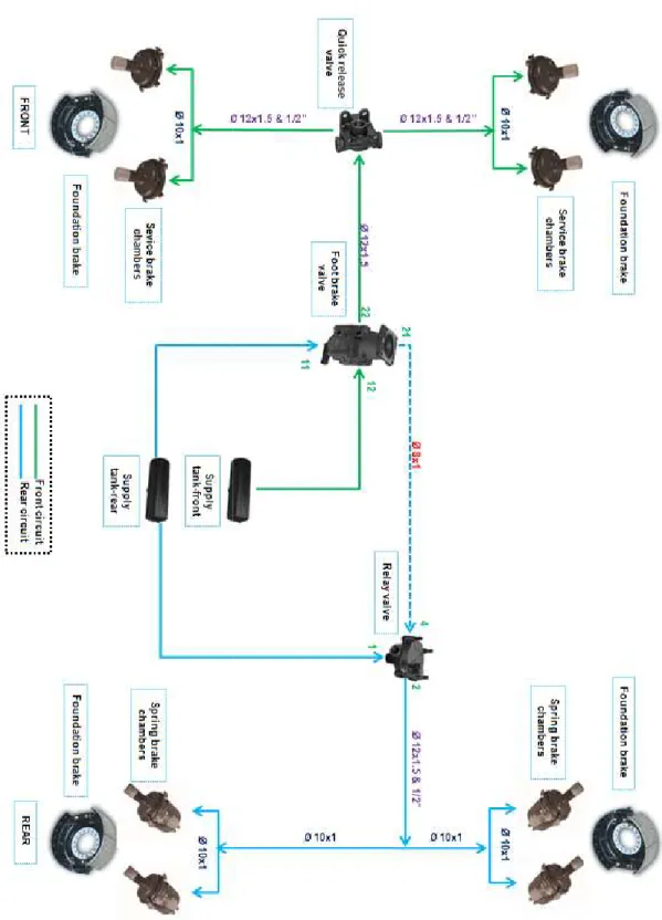
Before starting to model the pneumatic brake system, it is important to understand pneumatic service brake layout, usage and working principle of the components in the pneumatic brake system. Pneumatic service brake system contains front and rear supply tanks, foot brake valve, relay valve, service and spring brake chambers, pneumatic pipelines and foundation brakes.
When the driver applies the brake by pressing the brake pedal, foot brake valve opens and compressed air in supply tanks travels from the supply ports (11 and 12) to the delivery ports (21 and 22) of the foot brake valve.
For the front circuit, the compressed air flows from the delivery port of foot brake valve (22) to the input port of the quick release valve. Quick release valve divides compressed air through pneumatic pipeline into the service brake chambers mounted on the front axle.
For the rear circuit, the compressed air travels from the rear circuit delivery port of foot brake valve (21) through signal pipeline to the control port of relay valve (4). It permits to flow compressed air from supply port (1) to the delivery port (2) of relay valve. Compressed air is divided by tee passing through pneumatic pipeline and reaches into the spring brake chambers mounted on the rear axle.
Pressure in the brake chamber is converted into the force, which is transmitted to the foundation brakes in order to generate braking torque.
Service brake system layouts are shown in Figure 1.1 and 1.2 belong to the heavy-duty vehicles, on which response time tests are conducted for the verification of the pneumatic brake system model; one of the vehicles is equipped with wedge drum brakes and serial production level; the other one is equipped with disc brakes and prototype level. This layout is the key feature in the modelling procedure of the air brake system, since the effects of all components within the pneumatic brake circuit must be integrated to the mathematical model to ensure that the model is a good prediction for the actual brake system.
Figure 1.1 : Pneumatic service brake layout with wedge
6
Figure 1.2
7
9 2. MATHEMATICAL MODEL
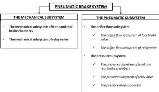
The pneumatic brake system consists of pneumatic and mechanical subsystems whose details are shown in Figure 2.1. Mechanical subsystem introduces the equations of motion related with the mechanical part of the brake system, while pneumatic subsystem deals with the dynamics of the compressible fluid, the air that is used in the brake system. Mathematical equations (2.1)-(2.25), which are used for mechanical and pneumatic subsystems are referenced from a book of Kluever, R. C., & Kluever, C. A. (2015).
Figure 2.1 : Mechanical and pneumatic subsystem details. 2.1 The Mechanical Subsystem
When driver presses the brake pedal, foot brake valve opens and the compressed air in front and rear air tanks travels through the front and rear circuits.
For the front circuit, compressed air in front supply tank flows into the brake chamber, which is mounted on the front axle. A piston force is generated depending on pressure increase in the brake chamber and it moves the push rod to actuate the foundation brake.
For the rear circuit, compressed air in rear supply tank travels through the signal pipeline into the control port of the relay valve. Pressure increased at the control port of the relay valve moves the relay piston and it permits the compressed air to flow
10
from supply port of relay valve into the rear brake chamber. Pressure in the brake chamber moves the push rod to actuate foundation brake, which is mounted on the rear axle.
The mechanical subsystem can also be classified into two subsystems. 2.1.1 The mechanical subsystem of front and rear brake chambers
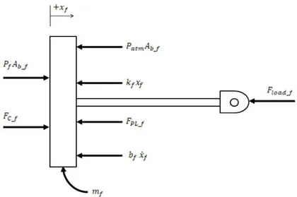
Figure 2.2 and 2.3 shows a free-body diagram of mechanical subsystem of front and rear brake chambers, which are composed of push rod mass, the air pressure forces, the seat contact force, the viscous friction force, the spring force with pre-load and the reactive load force due to spring in the foundation brake.
Figure 2.2 : Free-body diagram of mechanical subsystem of front brake chamber.
Figure 2.3 : Free-body diagram of mechanical subsystem of rear brake chamber.
11
Applying Newton’s second law, the motion equations of mechanical subsystems can be written for front and rear brake chambers as,
∑ F = P A _ + F _ − P A _ − k x − F _ − b x − F _ = m x (2.1) ∑ F = P A _ + F _ − P A _ − k x − F _ − b x − F _ = m x (2.2) 2nd order equations can be rewritten by rearranging equations (2.1) and (2.2),
m x + b x + k x = (P − P )A _ + F _ − F _ − F _ (2.3) m x + b x + k x = (P − P )A _ + F _ − F _ − F _ (2.4)
where,
m , m : Piston/ push rod masses b , b : Viscous friction coef icients k , k : Return spring constants P , P : Brake chamber pressures P : Atmospheric pressure
A _, A _ : Diaphragm cross sectional areas F _, F _ : Seat contact forces
F _, F _ : Pre load spring forces
F _, F _ : Load forces of foundation brakes x , x : Piston/push rod positions
x , x : Piston/push rod velocities x , x : Piston/push rod accelerations
The contact force only exists when the pre-load spring force F _ exceeds differential pressure force (P − P )A _. In this case, the piston is observed to be seated with x = 0. On the other hand, when differential pressure force (P − P )A _ exceeds pre-load spring force F _ or x > 0 then the contact force equals
to zero. Same condition is valid for rear brake chamber. This situation is described in equations (2.5) and (2.6).
12
F _ = F 0 if F_ − (P − P )A _ if F _ > (P − P )A _ and x = 0
_ ≤ (P − P )A _ or x > 0 (2.5)
F _ = F _ − (P − P )A _ if F _ > (P − P )A _ and x = 0 0 if F _ ≤ (P − P )A _ or x > 0 (2.6)
2.1.2 The mechanical subsystem of relay valve
Figure 2.3 shows a free-body diagram of mechanical subsystem of relay valve, which is composed of relay piston mass, the pressure force of control port, the seat contact force, the viscous friction force and the spring force with pre-load.
Figure 2.4 : Free-body diagram of mechanical subsystem of relay valve. Applying Newton’s second law, the equation of mechanical subsystem can be written for relay valve as,
∑ F = P A _ + F _ − k x − F _ − b x = m x (2.7)
2nd order equation can be rewritten by rearranging equation (2.7),
m x + b x + k x = P A _ + F _ − F _ (2.8)
where,
m : Relay piston mass
b : Viscous friction coef icient of relay valve k : Return spring constant of relay valve P : Control port pressure of relay valve
13 A _ : Cross sectional area of relay piston F _ : Seat contact force of relay valve F _ : Pre load spring force of relay valve
x : Relay piston position x : Relay piston velocity x : Relay piston acceleration
The contact force only exists when the pre-load spring force F _ exceeds pressure
force P A _ . In this case, the piston is observed to be seated with x = 0. On the other hand, when pressure force P A _ exceeds pre-load spring force F _ or x > 0 then the contact force equals to zero. This situation is described in equation (2.9).
F _ = 0 if FF _ − P A _ if F _ > P A _ and x = 0
_ ≤ P A _ or x > 0 (2.9)
2.2 The Pneumatic Subsystem
The pneumatic subsystem includes the front and rear supply tank pressures, which are connected to the front and rear brake chambers passing through the foot brake valve, the relay valve (for rear circuit only) and the pneumatic pipelines. Pressing the brake pedal opens the foot brake valve. The foot brake valve modulates highly pressurized air flow from the front and rear supply tanks to the front brake chamber and control port of relay valve. Exceeding the threshold pressure of control port opens relay valve. The relay valve modulates compressed air from rear supply tank to the rear brake chamber. Brake chamber pressure alters with the change of mass flow rate and chamber volume, which is dependent to the push rod stroke.
The pneumatic subsystem can also be classified into three subsystems. 2.2.1 The orifice flow subsystem
2.2.1.1 The orifice flow subsystem of foot brake valve
Mass-flow rates of the foot brake valve front and rear circuit deliveries are modelled by the orifice flow equations, which are given below for “chocked” and “unchocked flow” conditions depending on ratios of downstream to upstream pressure.
14 w = C A P (γ γ) γ− γ γ if > C (unchocked) (2.10) w = C A P γ C γγ if ≤ C (chocked) (2.11) w = C A P (γ γ) γ− γ γ if > C (unchocked) (2.12) w = C A P γ C γγ if ≤ C (chocked) (2.13) where,
w , w : Mass low rates
C : Discharge coef icient of FBV A : Ori ice cross sectional area of FBV P : Steady state system pressure γ: Ratio of speci ic heats (γ = 1.4) R: Gas constant
T: Air temperature C : Critical pressure ratio
Critical pressure ratio can be written as a function of ratio of specific heats,
C (2.14)
The critical pressure ratio is equal to 0.528 for air. When ratio of the downstream to upstream pressure (i.e. ratio of P to P for front circuit) is greater than the critical pressure ratio, then subsonic “unchocked flow” occurs at the valve orifice. On the other side when the critical pressure ratio of air is greater than the ratio of downstream to upstream pressure, then sonic (Mach 1) “chocked flow” involves at the valve orifice.
15 2.2.1.2 The orifice flow subsystem of relay valve
Mass-flow rate of relay valve is modelled by the orifice flow equations, which are given below for “chocked” and “unchocked flow” conditions depending on ratios of downstream to upstream pressure.
w = C _ A _ P γ (γ ) γ− γ γ if > C (unchocked) (2.15) w = C _ A _ P γ C γγ if ≤ C (chocked) (2.16) where,
w : Mass low rate of relay valve C _ : Discharge coef icient of relay valve A _ : Ori ice cross sectional area of relay valve 2.2.2 The pressure subsystem
2.2.2.1 The pressure subsystem of front and rear brake chambers
Using basic modelling equation for pneumatic system, 1st order pressure equations can be written for front and rear brake chambers as,
P = w − V (2.17)
P = w − V (2.18)
where,
P , P : Pressure rates
n: Exponent of polytropic expansion process V , V : Volumes of brake chambers
Exponent of polytrophic expansion process is assumed as value of n = 1 because of isothermal process.
Brake chamber volumes can be written as function of push rod positions x and x ,
16
V = V _ + A _ x (2.20)
where V _ and V_ are the volumes when push rod positions x = 0 and x = 0. Time derivatives of brake chamber volumes can be written as function of push rod velocities x and x ,
V = A _ x (2.21)
V = A _ x (2.22)
2.2.2.2 The pressure subsystem of relay valve
1st order pressure equation of relay valve is given below.
P = w − V (2.23)
where,
P : Pressure rate of control chamber V : Control chamber volume of relay valve
Control chamber volume of relay valve can be written as function of relay piston position x ,
V = V_ + V + A _ x (2.24)
where,
V_ : Control chamber volume when x = 0
V : Volume of internal chamber of pipes in control line
Time derivative of control chamber volume can be written as function of relay piston velocity x ,
V = A _ x (2.25)
2.2.2.3 The pressure drop subsystem
Pressing the brake pedal opens the foot brake valve and pressurized air in front and rear supply tanks starts to fill the brake chambers, passing through pneumatic pipelines by increasing total amount of volume. Because of this reason, air pressure in front and rear supply tanks decreases until reaching the steady state pressure of the pneumatic brake system.
17
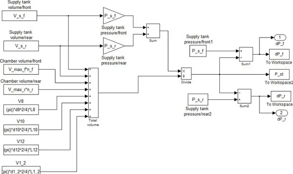
Applying Boyle’s gas law, the equation of pressure drop subsystem can be written as, P V + P V = P (V_ + V _ + n V _ + n V _ + V + V + V + V_ )
(2.26) where,
P_: Front supply tank pressure P_ : Rear supply tank pressure V_: Front supply tank volume V_ : Rear supply tank volume
V _: Front brake chamber volume when x = x _
V _ : Rear brake chamber volume when x = x _
n : Number of brake chamber at front axle n : Number of brake chamber at rear axle V : Internal chamber volume of pipe ∅8x1 V : Internal chamber volume of pipe ∅10x1 V : Internal chamber volume of pipe ∅12x1.5 V_ : Internal chamber volume of pipe 1/2"
Pressure drop in front and rear circuits can be written as,
dP = P_ − P (2.27)
19 3. SIMULINK MODEL
In this study, Matlab Simulink software is used in order to construct and develop the complete pneumatic brake system model.
Figure 3.1 shows Simulink model of pneumatic brake system, which is developed according to the mathematical equations mentioned for mechanical and pneumatic subsystems in Chapter 2. Pneumatic front and rear circuits in service brake system layout are included into the model.
In complete system model, one of the system inputs is defined as a step function of driver’s brake pedal force F and the other inputs are defined as front and rear circuit’s supply pressures P_ and P _ , which are constant. Valve’s orifice cross
sectional area A is proportional to the driver’s brake pedal force F therefore; it is defined as a gain factor in Simulink model.
Mechanical and brake chamber pressure subsystem blocks are generated for front and rear brake chambers and relay valve.
Regarding the 2nd order equations of the mechanical subsystem of front and rear brake chambers, there are two state variables for each brake chamber. Those are push rod positions and their time derivatives; in other words x , x for front brake chamber and x , x for rear brake chamber. Brake chamber pressures P and P , providing actuation forces of the foundation brakes are the input variables.
In mechanical subsystem of relay valve; relay piston position x and relay piston velocity x are output variables and control port pressure of relay valve P is the single input.
Orifice flow subsystem blocks are constructed for foot brake and relay valves. In orifice flow subsystem of the foot brake valve; supply tank pressures P_ and P_ , orifice cross sectional area of foot brake valve A , front brake chamber pressure P , control port pressure of relay valve P , pressure drop in front and rear circuits dP and dP are input variables and mass flow rates w and w are output variables. In orifice flow subsystem of relay valve; rear supply tank pressure P_ , orifice cross sectional area of relay valve A _ , pressure drop in rear circuit dP and rear brake
20
chamber pressure P are input variables and mass flow rate of relay valve w is single output.
Pressure subsystem blocks are generated for front and rear brake chambers and relay valve. In pressure subsystem of front and rear brake chambers; brake chamber pressures P and P are defined as output variables regarding the 1st order pressure
equation. Push rod positions x and x , push rod velocities x and x , mass flow rate of front circuit w and mass flow rate of relay valve w are input variables. Brake chamber volumes V and V and their time derivatives V and V are computed by using push rod positions x and x and push rod velocities x and x , which are given in equations (2.21) and (2.22).
In pressure subsystem of relay valve; mass flow rate of rear circuit w , relay piston position x , and its time derivative x are input variables and control port pressure of relay valve P is output variable. Control chamber volume V and its time derivative V are calculated by relay piston position x and relay piston velocity x .
When control port pressure of relay valve P exceeds its threshold value of P _
then orifice cross sectional area of relay valve switches zero to A _ therefore, a
switch block is added into the complete system model as a decision signal.
Regarding Boyle’s gas law equations of the pressure drop subsystem; there are two outputs, which are pressure drop in front and rear circuits dP and dP .
Figure 3.1
21
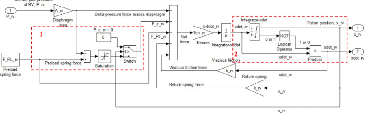
22 3.1 The Mechanical Subsystem Blocks
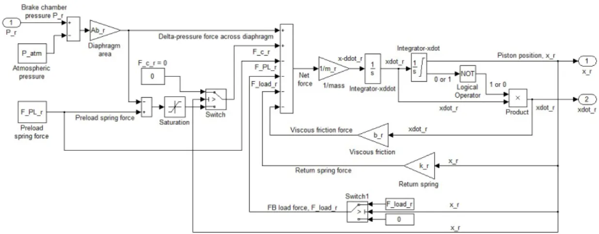
Mechanical subsystem blocks of front and rear brake chambers are constructed to introduce equations (2.3) and (2.4) into the model. Inner details of mechanical subsystem of front and rear brake chambers are shown in Figure 3.2 and 3.3.
First dashed box in Figure 3.2 shows contact force calculation, which is expressed in equation (2.5) and (2.6) for front and rear brake chambers. A saturation block is used for determining lower and upper limits of the difference between differential pressure force (P − P )A _ and pre-load spring force F _. The contact force F _ can only
take a positive value for this reason; lower limit of saturation block is defined as zero. The contact force F _ only exists when piston is seated or piston position is zero therefore, a switch block is added into the model as a decision signal.
Second dashed box in Figure 3.2 indicates the hard stop limit philosophy of push rod. Push rod displacement x cannot exceed maximum push rod displacement x _ because of full engagement of linings and disc or drum. When integrator output x has reached its limit x _ then push rod velocity x is equal to 0 and saturation
signal indicates a value of 1. Logical operator block is set to NOT operation and it converts the saturation signal from 1 to 0. This obtained output signal is multiplied by the velocity signal of the push rod x to produce push rod velocity information for being used in the simulation. On the other hand, when integral has not reached its limit then saturation signal is equals to 0 and it is converted from 0 to 1 by NOT operation.
The load force of the foundation brake F _ only exists when push rod displacement is greater than zero. For this reason, a switch is added to the mechanical subsystem of front brake chamber that is shown as third dashed box in Figure 3.2.
23
Figure 3.2 : Mechanical subsystem of front brake chamber.
Figure 3.3 : Mechanical subsystem of rear brake chamber.
Mechanical subsystem block of relay valve is constructed for the integration of equation (2.8) to the model. Inner details of mechanical subsystem of relay valve are shown in Figure 3.4.
First dashed box in Figure 3.4 shows contact force calculation, which is expressed in equation (2.9) for relay valve. A saturation block is used for determining lower and upper limits of the difference between pressure force P A _ and pre-load spring force F _ . The contact force F _ can only take a positive value, for this reason, lower limit of saturation block is defined as zero. The contact force F _ only exists when piston is seated or piston position is zero therefore, a switch block is added into the model as a decision signal.
Second dashed box in Figure 3.4 indicates the hard stop limit philosophy of relay piston. Relay piston displacement x cannot exceed maximum relay piston displacement x _ . When integrator output x has reached its limit
x _ , then relay piston velocity x is equal to 0 and saturation signal indicates a
1
2
24
value of 1. Logical operator block is set to NOT operation and it converts the saturation signal from 1 to 0. This obtained output signal is multiplied by the velocity signal of the relay piston x to produce relay piston velocity information for being used in the simulation. On the other hand, when integral has not reached its limit then saturation signal is equals to 0 and it is converted from 0 to 1 by NOT operation.
Figure 3.4 : Mechanical subsystem of relay valve. 3.2 The Pneumatic Subsystem Blocks
3.2.1 The orifice flow subsystem blocks
Details of orifice flow subsystem of foot brake valve are shown in Figure 3.5. Interpreted MATLAB Fcn blocks are defined to calculate mass flow rate of front and rear circuits w and w for chocked and unchocked flow conditions. For this purpose, customized M-files Valve_front.m and Valve_rear.m are generated by using equations (2.10)-(2.14). Foot brake valve is actuated by pressing the pedal and due to this action; predominance is occurred between front and rear circuit deliveries depending on the characteristic curve of valve. When control port pressure of relay valve P is greater than predominance pressure value of foot brake valve P , then orifice cross sectional area of the front circuit switches zero to A . For this reason, a switch block is added to the orifice flow subsystem of foot brake valve.
2 1
25
Figure 3.5 : Orifice flow subsystem of foot brake valve.
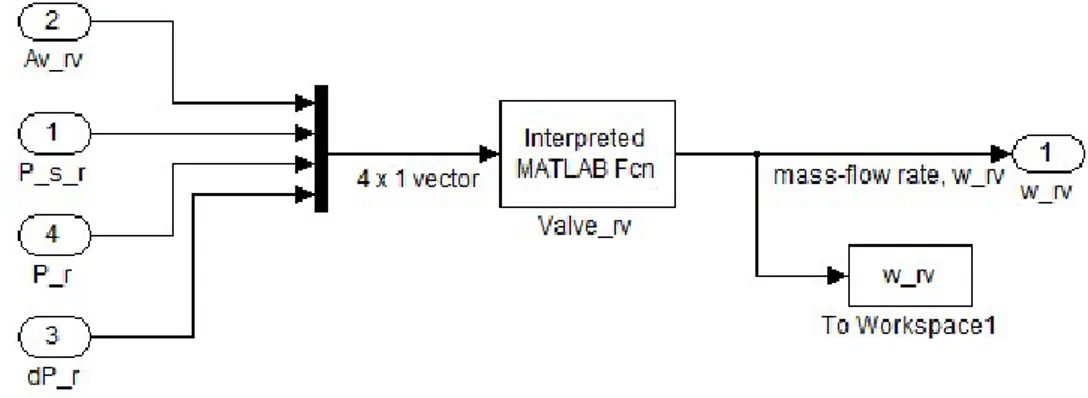
Details of orifice flow subsystem of relay valve are shown in Figure 3.6. Interpreted MATLAB Fcn block is defined to calculate mass flow rate of relay valve w therefore, customized M-file Valve_rv.m is generated by using equations (2.14)-(2.16).
Figure 3.6 : Orifice flow subsystem of relay valve. 3.2.2 The pressure subsystem blocks
Figure 3.7 and 3.8 show the inner details of pressure subsystem blocks of front and rear brake chambers. User defined Interpreted MATLAB Fcn blocks are added by
26
using customized M-files Pdot_front.m and Pdot_rear.m; which contain pressure rate, volume and volume rate equations (2.17)-(2.22).
Figure 3.7 : Pressure subsystem of front brake chamber.
Figure 3.8 : Pressure subsystem of rear brake chamber.
Inner details of pressure subsystem block of relay valve are shown in Figure 3.9. User defined Interpreted MATLAB Fcn block is added and customized M-files Pdot_rv.m is generated by related equations (2.23)-(2.25).
Figure 3.9 : Pressure subsystem of relay valve.
Pressure drop subsystem block is constructed for definition of equations (2.26)-(2.28) into the model. Inner details of pressure drop subsystem are shown in Figure 3.10.
27
29 4. EXPERIMENTAL STUDY
In this chapter, two response time tests are conducted; one for identification of the system parameters and the other for validation of the Simulink model. Tests are performed on two different heavy-duty vehicles given the details below.
4.1 Test-1: Serial Production Vehicle
Test-1 is conducted on the serial production vehicle whose air system’s working pressure is equal to 8 bars. The vehicle is equipped with the wedge drum brakes. Test-1 is performed to identify and define the unknown system parameters (orifice cross sectional areas of FBV and RV, threshold pressure of RV etc.) that cannot be obtained from the technical datasheets of the air brake system components.
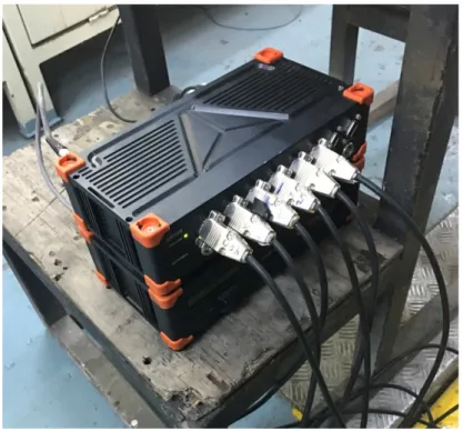
In order to get the response time measurements of the vehicle equipped with drum brakes, DEWESoft SIRIUSi 8xSTGM data acquisition system is installed on the vehicle as shown in Figure 4.1 below.
Figure 4.1 : Data acquisition system.
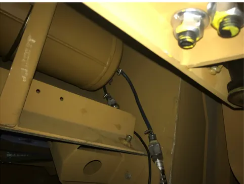
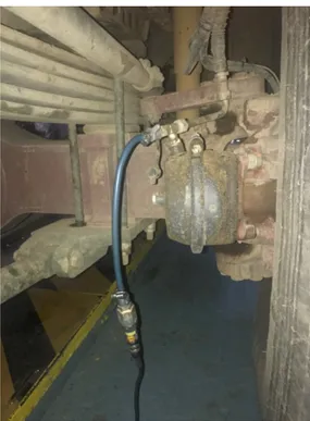
To measure brake chamber pressure transients, two Keller PR-23 SY (0-10 bar and 0-5V) pressure sensors are mounted on the brake chambers that are located at the front axle left and rear axle right as shown in Figure 4.2 and Figure 4.3.
30
Figure 4.2 : Pressure sensor mounted on the front axle left.
Figure 4.3 : Pressure sensor mounted on the rear axle right.
The other two pressure sensors are fitted on the front and rear circuit deliveries of the foot brake valve (Port 22 and Port 21) to measure the time elapsing from the initiation of brake pedal actuation, see Figure 4.4.
31
Figure 4.4 : Pressure sensors fitted on the foot brake valve.
In addition to these, two more pressure sensors are fitted on the air tanks for the purpose of monitoring front and rear tank pressures as shown in Figure 4.5.
Figure 4.5 : Pressure sensors mounted on the front and rear tanks.
All the 6 pressure sensors are connected to the DEWESoft SIRIUSi 8xSTGM data acquisition system via 6 channels and the data acquisition system is also connected to the laptop computer. Thus, the test measurements can be monitored on the laptop computer in real time. The pressure information measured by Keller PR-23 SY pressure sensors is transferred to the DEWESoft SIRIUSi 8xSTGM data acquisition system. The DEWESoftX data acquisition software stores the data in DEWESoftX
32
data file format. Sampling rate is set to 2000 Hz from the DEWESoftX data acquisition software. Figure 4.6 shows the DEWESoftX user interface design, which is prepared and developed for this study. The pressure information that is read by all the 6 pressure sensors depending on the elapsed time can be monitored from the digital indicators, which located on the DEWESoftX user interface.
Before the response time test, it is necessary to define cut-in pressure of the air compressor on the vehicle because at the beginning of the response time test, the pressure in the front and rear tanks must be equal to the cut-in pressure of air compressor.
Here, response time is defined as the elapsed time measured from the instant that actuation of the brake pedal is started to the instant that the pressure in the brake chamber reaches to 75% of the cut-in pressure of the air compressor (UN, 2014). In order to define cut-in pressure of the air compressor, the following steps are taken into consideration;
1. Start the measurement and recording by using DEWESoftX software.
2. Start the engine and ensure that the vehicle is stationary and running at the idle speed.
3. Wait until the pressures in the air tanks reach cut-off pressure of air compressor. 4. Press the brake pedal at half stroke and monitor the pressure decreased in the air tanks.
5. Repeat step 4 until the pressures in the air tanks increase again (cut-in pressure of air compressor).
6. Stop data logging and review the results.
It can be seen in Figure 4.7 that the cut-in pressure of air compressor is obtained a value of 7.3 bars. Thus, 75% of the cut-in pressure of the air compressor is calculated 5.5 bars for response time determination.
Figure 4.6 : Cut
The response time test procedure
1. Start the measurement by using DEWESoftX. 2. Start the engine.
3. Release the hand brake valve.
4. Ensure that the vehicle is stationary and running at the idle speed. 5. Wait until the pressure
6. Stop the engine.
7. Press the brake pedal at half stroke and monitor the pr tanks.
8. Repeat step 7 until the pressure air compressor.
9. Start recording the test by using DEWESoftX. 10. Press the brake pedal at full stroke immediately. 11. Hold the brake pedal at the end of the pedal travel 12. Release the brake pedal immediately.
33
Cut-in pressure of compressor of serial production vehicle. The response time test procedure is as follows;
Start the measurement by using DEWESoftX.
hand brake valve.
the vehicle is stationary and running at the idle speed.
Wait until the pressures in the air tanks reach cut-off pressure of air compressor.
Press the brake pedal at half stroke and monitor the pressure decrease
step 7 until the pressures in the air tanks is equal to the cut
Start recording the test by using DEWESoftX. Press the brake pedal at full stroke immediately.
rake pedal at the end of the pedal travel. Release the brake pedal immediately.
serial production vehicle.
the vehicle is stationary and running at the idle speed.
off pressure of air compressor.
essure decreased in the air
34 13. Stop data logging and review the results.
According to European Braking Regulation UNECE R13, following requirements must be achieved (UN, 2014).
• In order to obtain a succeeded actuation in the response time test, the pressure at the front and rear circuit deliveries of the foot brake valve must reach at some specific percentage of its asymptotic/final value at the corresponding time instants. These specific percentages and related time instants are given in Table 4.1.
• For an actuating time of 0.2 seconds, response time should not exceed 0.6 s and response time measurement results should be rounded to the nearest tenth of a second.
Table 4.1 : Requirements of a succeeded actuation (UN, 2014).
.. (%) of asymptotic/final value Elapsed time (s)
10 0.2
75 0.4
Figure 4.7 shows response time test results of serial production vehicle. It can be seen that final pressure at the front and rear circuit deliveries of the foot brake valve is equal to 6.6 bars.
Here, the elapsed time measured from the actuation of brake pedal to the time that the pressure reaches to 10% of final pressure of the front delivery is equal to t =0.02 s. As for the rear delivery, the elapsed time is monitored as t =0.01 s. For the second requirement of a succeeded actuation, the elapsed time measured from the actuation of brake pedal to the time that the pressure reaches to 75% of final pressure of the front delivery is equal to t =0.4 s. As for the rear delivery, the elapsed time is monitored as t =0.1 s. Therefore, results of response time test fulfill the requirements of a succeeded actuation.
For the response time determination, 75% of the cut-in pressure of the air compressor is obtained 5.5 bars. At this point, response time results of front and rear brake chambers are obtained as t =0.6 s and t =0.5 s respectively. Hence, it can be concluded that for the given test requirements response time results of front and rear circuits stay within regulation limits.
Figure 4.7
4.2 Test-2: Prototype Vehicle
Test-2 is performed on the prototype 10 bars. The vehicle is
verification and validation of pneumatic
constructed and developed in this study to predict response time of the system. For this purpose, DEWESoft SIRIUSi 8xSTGM data acquisition sy
installed on the vehicle. As mentioned in Test
DEWESoft SIRIUSi 8xSTGM data acquisition system. Two pressure sensors (Keller PR-23 SY 0
brake chambers’
shown in Figure 4.8 and Figure 4.9
front and rear circuit deliveries of the foot brake valve (Port 22 and Port 21), see Figure 4.10. Furthermore, two pressure sensors
the front and rear tank Figure 4.11.
35
Figure 4.7 : Response time test results of serial production vehicle. 2: Prototype Vehicle
performed on the prototype vehicle whose working pressure is equal to . The vehicle is equipped with the disc brakes. Test-2 is
and validation of pneumatic brake system
constructed and developed in this study to predict response time of the system. For this purpose, DEWESoft SIRIUSi 8xSTGM data acquisition sy
installed on the vehicle.
s mentioned in Test-1, all the 6 pressure sensors are
DEWESoft SIRIUSi 8xSTGM data acquisition system. Two pressure sensors 23 SY 0-10 bar and 0-5 V) that are used to measure t
pressures located at the front axle left and rear a shown in Figure 4.8 and Figure 4.9. Other two pressure sensors
front and rear circuit deliveries of the foot brake valve (Port 22 and Port 21), see . Furthermore, two pressure sensors, which are used for monitoring the front and rear tank pressures, are mounted on the air tanks, as shown in
serial production vehicle.
ehicle whose working pressure is equal to is conducted for the brake system model, which is constructed and developed in this study to predict response time of the system. For this purpose, DEWESoft SIRIUSi 8xSTGM data acquisition system is
connected to the DEWESoft SIRIUSi 8xSTGM data acquisition system. Two pressure sensors used to measure the front and rear located at the front axle left and rear axle left as . Other two pressure sensors are fitted on the front and rear circuit deliveries of the foot brake valve (Port 22 and Port 21), see e used for monitoring r tanks, as shown in
36
Figure 4.8 : Pressure sensor mounted on the front axle left of prototype vehicle.
37
Figure 4.10 : Pressure sensors mounted on the foot brake valve of prototype vehicle.
Figure 4.11 : Pressure sensors mounted on the front and rear tanks of prototype vehicle.
Cut-in pressure of air compressor is obtained as 8.8 bars by repeating test for the prototype vehicle using cut-in pressure determination procedures mentioned in Section 4.1, see Figure 4.12.
Response time test of the prototype vehicle equipped with disc brakes is conducted by using response time test procedure mentioned in Section 4.1. Response time test results are shown in Figure 4.13 below.
Figure 4.12 :
Cut-Figure 4.13 : Response time test result
It can be seen that final pressure at the front and rear circuit deliveries of the foot brake valve is equal to 7.8 bars. Thus, the elapsed time measured from the actuation of brake pedal to the time that the pressure reaches to 10
38
-in pressure of compressor of prototype vehicle.
Response time test results of prototype vehicle.
It can be seen that final pressure at the front and rear circuit deliveries of the foot brake valve is equal to 7.8 bars. Thus, the elapsed time measured from the actuation that the pressure reaches to 10% of final pressure of the
in pressure of compressor of prototype vehicle.
It can be seen that final pressure at the front and rear circuit deliveries of the foot brake valve is equal to 7.8 bars. Thus, the elapsed time measured from the actuation pressure of the
39
front delivery is equal to t =0.07 s. As for the rear delivery, the elapsed time is monitored as t =0.07 s.
For the second requirement of a succeeded actuation, the elapsed time measured from the actuation of brake pedal to the time that the pressure reaches to 75% of final pressure of the front delivery is equal to t =0.3 s. As for the rear delivery, the elapsed time is monitored as t =0.1 s. It is shown that results fulfill requirements of a succeeded actuation for the response time test.
It can be calculated that 75% of the cut-in pressure of the air compressor is 6.6 bars. At this point, response time results of front and rear brake chambers are obtained as t =0.9 s and t =0.5 s respectively. Hence, it can be concluded that for the given test requirements, response time results of front circuit could not pass the test.
41 5. RESULTS AND DISCUSSION
In this chapter, analyses are performed by using system model, which is obtained from Chapter 3. Analysis results are verified by using experimental data taken from the vehicle tests that are done in Chapter 4. For providing system improvements, a study is conducted in which possible design alternatives are discussed on the prototype vehicle.
5.1 Analysis and Verification of the System Model
In this section, two response time analyses are conducted for the validation of the system model by using system parameters of two different heavy-duty vehicles given the details below.
5.1.1 Analysis-1: Serial Production Vehicle 5.1.1.1 System parameters of Analysis-1
In this section, analyses of the pneumatic brake system model that is constructed in Chapter 3 are performed by using system parameters of serial production vehicle, which is equipped with wedge drum brakes. Most of the system parameters are obtained from the technical datasheets of the air brake system components and from similar studies in the current literature. The other unknown system parameters will be identified in this section by using response time test of the serial production vehicle (Test-1) whose details and results are given in section 4.1. For the analysis of the serial production vehicle, defined system parameters are summarized in Table 5.1 and the details are given below.
Viscous friction coefficients (b , b and b ) and return spring constants (k , k and k ) are taken from similar studies in current literature (Kluever & Kluever, 2015; Yi et al., 2015). Maximum push–rod strokes (x _ and x _ ) are taken a
value of 0.027m for wedge brake with unworn linings. Other brake chamber parameters like piston/push rod masses (m and m ), pre-load spring forces (F _
42
and F _ ), diaphragm cross-sectional areas (A _ and A _ ), initial and maximum chamber volumes (V _, V_ ,V _ and V _ ) are obtained from technical drawings of front and rear brake chambers, which are showed in Appendix A.1 and A.2. For actuation purpose, two brake chambers should be mounted on a wedge brake, making in total four brake chambers for each axle. Load forces of foundation brakes (F _ and F _ ) are obtained from standard brake system calculations of a 6x6 heavy-duty truck, on which same wedge brakes are used.
Discharge coefficient of foot brake valve (C ) is taken from similar study in literature, in which the same foot brake valve is used for regulating the compressed air (Selvaraj et al., 2014). Same value is taken into consideration for discharge coefficient of relay valve (C _ ). Predominance pressure (P ) is obtained from
datasheet of foot brake valve shown in Appendix A.3.
Pre-load spring force of relay valve (F _ ), maximum relay piston stroke (x _ )
and cross sectional area of relay piston (A _ ) are referenced from similar studies. It is observed from the results of Test-1 that, when the pressure at rear circuit delivery of the foot brake valve (Port 21) exceeds to its asymptotic/final value then the pressure at the rear brake chambers start increasing from zero. Therefore, the threshold pressure of relay valve (P _ ) is assumed to be equal to the steady state system pressure (P ).
Pneumatic pipeline dimensions are determined according to the pneumatic service brake system layout of serial production vehicle.
Supply tank pressures are set to the value of 7.427(105) Pa, which is obtained from the result of Test-1, measured as compressor cut-in pressure.
Experimental pressure curves of front and rear brake chambers (P_ and P_ )
obtained from Test-1 are introduced to the Simulink model. These experimental results are plotted together with the numerical brake chamber pressure transients (P and P ). In order to identify unknown orifice cross sectional areas of FBV and RV, a series of analyses are conducted under nominal operating conditions by changing both orifice area values until the numerical pressure curves are fitted to the experimental pressure curves, see Figure 5.1. Also, actuation time of the brake pedal is set to 0.04 s for the purpose of curve fitting.