Compressive Diffusion Strategies Over Distributed
Networks for Reduced Communication Load
Muhammed O. Sayin and Suleyman Serdar Kozat, Senior Member, IEEE
Abstract—We study the compressive diffusion strategies over
distributed networks based on the diffusion implementation and adaptive extraction of the information from the compressed dif-fusion data. We demonstrate that one can achieve a comparable performance to the full information exchange configurations, even if the diffused information is compressed into a scalar or a single bit, i.e., a tremendous reduction in the communication load. To this end, we provide a complete performance analysis for the compressive diffusion strategies. We analyze the transient, the steady-state and the tracking performances of the configu-rations in which the diffused data is compressed into a scalar or a single-bit. We propose a new adaptive combination method improving the convergence performance of the compressive dif-fusion strategies further. In the new method, we introduce one more freedom-of-dimension in the combination matrix and adapt it by using the conventional mixture approach in order to enhance the convergence performance for any possible combination rule used for the full diffusion configuration. We demonstrate that our theoretical analysis closely follow the ensemble averaged results in our simulations. We provide numerical examples showing the improved convergence performance with the new adaptive com-bination method while tremendously reducing the communication load.
Index Terms—Compressed diffusion, distributed network,
per-formance analysis.
I. INTRODUCTION
D
ISTRIBUTED network of nodes provides enhanced performance for several different applications, such as source tracking, environment monitoring and source lo-calization [1]–[4]. In such a distributed network, each node encounters possibly a different statistical profile, which pro-vides broadened perspective on the monitored phenomena. In general, we could reach the best estimate with access to all ob-servation data across the whole network since the obob-servation of each node carries valuable information [5]. In the distributed adaptive estimation framework, we distribute the processing over the network and allow the information exchange among the nodes so that the parameter estimate of each node converges to the best estimate [4], [6].Manuscript received December 20, 2013; revised April 19, 2014 and July 21, 2014; accepted July 26, 2014. Date of publication August 14, 2014; date of current version September 04, 2014. The associate editor coordinating the review of this manuscript and approving it for publication was Dr. Hing Cheung So. This work was supported in part by the Outstanding Researcher Programme of Turkish Academy of Sciences and TUBITAK projects, Contract no: 112E161 and 113E517.
The authors are with the Department of Electrical and Electronics En-gineering, Bilkent University, Bilkent, Ankara 06800, Turkey (e-mail: [email protected]; [email protected]).
Color versions of one or more of the figures in this paper are available online at http://ieeexplore.ieee.org.
Digital Object Identifier 10.1109/TSP.2014.2347917
In the distributed architectures, one can use different ap-proaches to regulate the information exchange among nodes such as the diffusion implementations [6]–[11]. The generic diffusion implementation defines a communication protocol in which only the nodes from a certain neighborhood could exchange information with each other [1], [6]–[11]. In this framework, each node uses a local adaptive algorithm and im-proves its parameter estimation by fusing its information with the diffused parameter estimations of the neighboring nodes. Via this information sharing, the diffusion approach provides robustness against link failures and changing network topolo-gies [6]. However, diffusion of the parameter vectors within the neighborhoods results in high amount of communication load. For example, in a typical diffusion network of nodes the overall communication burden is given by where is the size of the diffused vector, which implies that the size of the diffused information has a multiplicative impact on the overall communication burden. Additionally, in a wireless network, the neighborhood size also plays a crucial role on the overall communication load since the larger the neighborhood is, the more power is required in the transmission of the information [1]–[4].
We study the compressive diffusion strategies that achieve a better trade-off in terms of the amount of cooperation and the required communication load [12]. Unlike the full diffu-sion configuration, the compressed diffudiffu-sion approach diffuses a single-bit of information or a reduced dimensional data vector achieving an impressive reduction in the communication load, i.e., from a full vector to a single bit or to a single scalar. The diffused data is generated through certain random projections of the local parameter estimation vector. Then, the neighboring nodes adaptively construct the original parameter estimations based on the diffused information and fuse their individual esti-mates for the final estimate. In this sense, this approach reduces the communication load in the spirit of the compressive sensing [12], [13]. The compression is lossy since we do not assume any sparseness or compressibility on the parameter estimation vector [13], [14]. However, the compressive diffusion approach achieves comparable convergence performance to the full dif-fusion configurations. Since the communication load increases far more in the large networks or the networks where the paths among the nodes are relatively longer, the compressive diffusion strategies play a crucial role in achieving comparable conver-gence performance with significantly reduced communication load.
There exist several other approaches that seek to reduce the communication load in distributed networks. In [15], [16] and [17], the authors propose the partial diffusion strategies where the nodes diffuse only selected coefficients of the parameter
es-1053-587X © 2014 IEEE. Personal use is permitted, but republication/redistribution requires IEEE permission. See http://www.ieee.org/publications_standards/publications/rights/index.html for more information.
timation vector. In [18], the dimension of the diffused informa-tion is reduced through the Krylov subspace projecinforma-tion tech-niques in the set-theoretic estimation framework. In [19], within a predefined neighborhood, the parameter estimate is quantized before the diffusion in order to avoid unlimited bandwidth re-quirement. In [20], the nodes transmit the sign of the innovation sequence in the decentralized estimation framework. In [21], in a consensus network, the relative difference between the states of the nodes is exchanged by using a single bit of information. As distinct from the mentioned works, the compressive diffu-sion strategies substantially compress the whole diffused infor-mation and extract the inforinfor-mation from the compressed data adaptively [12].
In this paper, we provide a complete performance analysis for the compressive diffusion strategies, which demonstrates com-parable convergence performance of the compressed diffusion to the full information exchange configuration. We note that studying the performance of distributed networks with compres-sive diffusion strategies is not straight-forward since adaptive extraction of information from the diffused data brings in an additional adaptation level. Moreover, such a theoretical anal-ysis is rather challenging for the single-bit diffusion strategy due to the highly nonlinear compression. However, we analyze the transient, steady-state and tracking performance of the config-urations in which the diffused data is compressed into a scalar or a single-bit. We also propose a new adaptive combination method improving the performance for any conventional com-bination rule. In the compressive diffusion framework, we fuse the local estimates with the adaptively extracted information from substantially compressed diffusion data. The extracted in-formation carries relatively less inin-formation than the original data. Hence, we introduce “a confidence parameter” concept, which adds one more freedom-of-dimension in the combina-tion matrix. The confidence parameter determines how much we are confident with the local parameter estimation. Through the adaptation of the confidence parameter, we observe enormous enhancement in the convergence performance of the compres-sive diffusion strategies even for relatively long filter lengths.
Our main contributions include: 1) for Gaussian regressors, we analyze the transient, steady-state and tracking performance of scalar and single-bit diffusion techniques; 2) We demonstrate that our theoretical analysis accurately models the simulated results; 3) We propose a new adaptive combination method for compressive diffusion strategies, which achieves a better trade-off in terms of the transient and steady state performance; 4) We provide numerical examples showing the enhanced convergence performance with the new adaptive combination method in our simulations.
We organize the paper as follows. In Section II, we ex-plain the distributed network and diffusion implementation. In Section III, we introduce the compressive diffusion strategy, i.e., reduced-dimension and single-bit diffusion. In Section IV, we provide a global recursion model for the deviation pa-rameters to facilitate the performance analysis. For Gaussian regressors, we analyze the mean-square convergence per-formance of the scalar and single-bit diffusion strategies in Sections V and VI, respectively. In Sections VII and VIII we analyze the steady-state and tracking performance of the scalar and single-bit diffusion approaches. In Section IX, we introduce
the confidence parameter and propose a new adaptive com-bination method, improving the convergence performance of the compressive diffusion strategies. In Section X, we provide numerical examples demonstrating the match of theoretical and simulated results, and enhanced convergence performance with the new adaptive combination technique. We conclude the paper in Section XI with several remarks.
Notation: Bold lower (or upper) case letters denote column
vectors (or matrices). For a vector (or matrix ), (or ) is its ordinary transpose. and denote the norm and the weighted norm with the matrix , respectively (provided that is positive-definite). We work with real data for nota-tional simplicity. For a random variable (or vector ), (or ) represents its expectation. Here, denotes the trace of the matrix . The operator produces a column vector or a matrix in which the arguments of are stacked one under the other. For a matrix argument, operator constructs a diagonal matrix with the diagonal entries of and for a vector argument, it creates a diagonal matrix whose diag-onal entries are elements of the vector. The operator takes the Kronecker tensor product of two matrices.
II. DISTRIBUTEDNETWORK
Consider a network of nodes where each node measures1
and related via the true parameter vector through a linear model
where denotes the temporally and spatially white noise. We assume that the regression vector is spatially and tempo-rally uncorrelated with the other regressors and the observation noise. If we know the whole temporal and spatial data overall network, then we can obtain the parameter of interest by minimizing the following global cost with respect to the param-eter estimate [6]:
(1) The stochastic gradient update for (1) leads to the global least-mean square (LMS) algorithm as
(2) where is the step size [7]. Note that (2) brings a sig-nificant communication burden by gathering the network-wise information in a central processing unit. Additionally, central-ized approach is not robust against link failures and changing network statistics [4], [6]. On the other hand, in the diffusion implementation framework, we utilize a protocol in which each node can only exchange information with the nodes from its neighborhood (with the convention ) [6], [7]. This protocol distributes the processing to the nodes and provides tracking ability for time-varying statistical profiles [6].
1Although we assume a time invariant unknown system vector , we also
provide the tracking performance analysis for certain non-stationary models later in the paper.
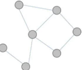
Fig. 1. Distributed network of nodes and the neighborhood .
Assuming the inner-node links are symmetric, we model the distributed network as an undirected graph where the nodes and the communication links correspond to its vertices and edges, respectively (See Fig. 1). In the distributed network, each node employs a local adaptation algorithm and benefits from the in-formation diffused by the neighboring nodes in the construc-tion of the final estimate [6]–[9]. For example, in [6], nodes
dif-fuse their parameter estimate to the neighboring nodes and each
node performs the LMS algorithm given as
(3) where is the local step-size. The intermediate parameter vector is generated through
with ’s are the combination weights such that
for all . For a given network topology, the com-bination weights are determined according to certain combina-tion rules such as uniform [22], the Metropolis [23], [24], rela-tive-degree rules [8] or adaptive combiners [25].
We note that in (3) we could assign as the final estimate in which we adapt the local estimate through the local observation data and then we fuse with the diffused estimates to generate the final estimate. In [7], authors examine these approaches as combine-than-adapt (CTA) and adapt-than-combine (ATC) dif-fusion strategies, respectively. In this paper, we study the ATC diffusion strategy, however, the theoretical results hold for both the ATC and the CTA cases for certain parameter changes pro-vided later in the paper.
We emphasize that the diffusion of the parameter estimation vector also brings in high amount of communication load. In the next section, we introduce the compressive diffusion strategies enabling the adaptive construction of the required information from the reduced dimensional diffused information.
III. COMPRESSIVEDIFFUSION
We seek to estimate the parameter of interest through the
reduced dimension information exchange within the
neighbor-hoods. To this end, in the compressed diffusion approach, unlike the full diffusion scheme, we exchange a significantly reduced amount of information. The diffused information is generated through a certain projection operator, e.g., a time-variant vector , by linearly transforming the parameter vector, e.g., . In particular, node diffuses instead of the whole parameter vector in the scalar diffusion scheme. We might also use a projection matrix, e.g., , such that
or . Then the neighboring nodes of can generate an estimate of through the exchanged infor-mation by using an adaptive estiinfor-mation algorithm as explained later in this chapter and in [12]. We emphasize that the estimates ’s are the constructed information using the diffused infor-mation, not the actual diffused information. Hence, the diffused information might have far smaller dimensions than the param-eter estimation vector, which reduces the communication load significantly.
We note that the projection operator plays a crucial role in the construction of . Hence we constrain the projection op-erator to span the whole parameter space in order to avoid bi-ased estimate of the original parameters [12]. Bbi-ased on this constraint, we can construct the projection operator through the pseudo-random number generators (PRNG), which generates a sequence of numbers determined by a seed to approximate the properties of random numbers [26], or through a round-robin fashion in the sequential selection scheme as in [16].
Remark 3.1: We point out that the randomized projection
vector could be generated at each node synchronously provided that each node uses the same seed for the pseudo-random gener-ator mechanism [26]. Such seed exchanges and the synchroni-sation can be done periodically by using pilot signals without a serious increase in the communication load [27]. In Section X, we examine the sensitivity of the proposed strategies against the asynchronous events, e.g., complete loss of diffused infor-mation, in several scenarios through numerical examples.
Most of the conventional adaptive filtering algorithms can be derived using the following generic update:
(4) where is the divergence, distance or a priori knowl-edge, e.g., the Euclidean distance , and
is the loss function, e.g., the mean square error
[28], [29]. Correspondingly, the diffusion based distributed es-timation algorithms can also be generated through the update (4). However, note that the compressive diffusion scheme pos-sesses different side information about the parameter of interest from the full diffusion configuration, i.e., the constructed estimates instead of the original parameters. Although the con-structed estimates ’s track the original parameter estimation vectors, they are also parameter estimates of as the original parameters. Particularly, in the proposed schemes, each node has access to the a priori knowledge about the true parameter
vector as and ’s for . Hence, in the
com-pressive diffusion implementation, we update according to
(5) such that in the update we also consider the Euclidean distance with the local parameter estimation and the constructed estimates of the neighboring nodes. In order to simplify the
optimization in (5) and to obtain an LMS update exactly, we can replace the loss term with the first order Taylor series expansion around , i.e.,
(6)
where we denote . Similarly, the first
order Taylor series expansion around leads
(7)
where . Since , the
approx-imations (6) and (7) in (5) yields
(8) The minimized term in (8) is a convex function of and the Hessian matrix is positive definite. Hence, taking derivative and equating zero, we get the following update
(9) where
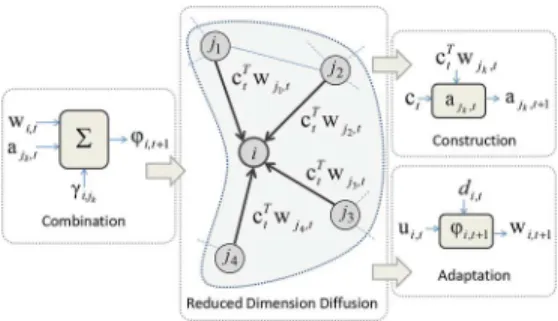
(10) which is similar to the distributed LMS algorithm (3). Note that if we interchange and , in other words, when we assign the outcome of the combination as the final estimate rather than the outcome of the adaptation, we have the following algorithm: (11) (12) We point out that (9) and (10) are the CTA diffusion strategy while (11) and (12) are the ATC diffusion strategy. Figs. 2 and 3 summarize the compressive diffusion strategy for the CTA and ATC strategies where . We next introduce different approaches to generate the diffused information (which are used to construct ’s).
In the compressive diffusion approach, instead of the full vector and irrespective of the final estimate, we always diffuse the linear transformation of the outcome of the adaptation, e.g., we diffuse in the CTA strategy and
in the ATC strategy. At each node, with the diffused information , we update the constructed estimate according to
Fig. 2. CTA strategy in the scalar diffusion framework.
Fig. 3. ATC strategy in the scalar diffusion framework.
where we choose the diffused data as the desired signal and try to minimize the mean-square of the difference between the
es-timate and . Here, ’s are the estimates of
the ’s or ’s in the CTA and the ATC strategies, respec-tively. The first order Taylor series approximation of the loss term around yields the following update
(13) where is the construction step size. We note that in [12] the reduced dimension diffusion approach constructs ’s through the minimum disturbance principle and resulted update involves as the normalization term. The constructed estimates ’s are combined with the outcome of the local adaptation algorithm through (10) or (12).
We next introduce methods where the information exchange is only a single bit [12]. When we construct at node , as-suming ’s are initialized with the same value, node has knowledge of the constructed estimate . Hence, we can perform the construction update at each neighboring node via the diffusion of the estimation error, i.e., . Note that this does not influence the communication load, however, through the access to the exchange estimate we can fur-ther reduce the communication load. Using the well-known sign algorithm [5], we can construct as
(14) Hence, we can repeat (14) at each neighboring node via the dif-fusion of only and then we combine with the local estimate by using (10) or (12).
In Table I, we tabulate the description of the proposed algo-rithms. We note that as seen in the Table I, the construction of requires additional updates at each neighboring nodes.
TABLE I
THEDESCRIPTION OF THECOMPRESSIVEDIFFUSIONSCHEMES
WITH THEATC STRATEGY
However, in the following, we propose an approach signifi-cantly reducing this computational load provided that all nodes use the same projection operator. We note that (9) and (11) re-quire the linear combination of the constructed estimates. To this end, we define
so that for the same step size, i.e., , the following relations
.. .
can be rewritten in a single update as
(15) In that sense, as an example, instead of (12), we can construct the final parameter estimate through
(16) thanks to the linear error function in the LMS update. Hence, we can significantly reduce the computational load, i.e., to only an additional LMS update, in the scalar diffusion strategies through (15) and (16). On the other hand, if the sign algorithm is used at each node in the construction of , each node should construct ’s separately since the sign algorithm has a nonlinear error update, i.e., . However, the sign algorithm is known for its low complexity implementation and can be implemented through shift-registers provided that the step-size is chosen as a power of 2 [5]. In this sense, the single-bit diffusion strategy sig-nificantly reduces the communication load, i.e., from continuum to a single bit, with a relatively small computational complexity increase. We point out that the single-bit diffusion also over-comes the bandwidth related issues especially in the wireless networks due to the significant reduction in the communication load and the inherently quantized diffusion data.
In the sequel, we introduce a global model gathering all net-work operations into a single update.
IV. GLOBALMODEL
We can write the scalar (13) and single bit (14) diffusion ap-proaches for the ATC diffusion strategy in a compact form as
(17) (18)
where and . For
scalar and single bit diffusion approaches, and , respectively.
For the state-space representation that collects all net-work operations into a single update, we define
with dimensions and
with dimensions. For a
given combination matrix , we denote .
Additionally, the regression and projection vectors yields the following global matrices
..
. . .. ... ... . .. ...
Indeed, we can model the network with compressive diffusion strategy as a larger network in which each node has an imagi-nary counterpart which diffuses to the neighbors of , which
is similar to the full diffusion configuration. The real nodes only get information from the imaginary nodes and do not diffuse any information. In that case, the network can be modelled as a directed graph with asymmetric inner node links and the com-bination matrix is given by
where and . Then, we can write
in terms of and as
(19)
where and . The state-space
representation is given by
(20) where
, and .
We obtain the global deviation vectors as
(21)
Since ,
(22) then the global deviation update yields
(23) (24) In (25),
(25) we represent the global deviation updates (23) and (24) in a single equation or equivalently
(26)
where . We next use the following
assump-tions in the analyses of the weighted-energy recursion of (26):
Assumption 1:
The regressor signal is zero-mean independently and identically distributed (i.i.d.) Gaussian random vector process and spatially and temporally independent from the other regressor signals, the randomized projection operator and the observation noise. Each node uses spa-tially and temporally independent projection vector, i.e.,
. The projection operator is zero-mean i.i.d. Gaussian random vector process and the observation noise is also a zero-mean i.i.d. Gaussian random variable. Note that such assumptions are commonly used in the analysis of traditional adaptive schemes [5], [30].
Assumption 2:
The a priori estimation error vector in the construction up-date (20), i.e., , has Gaussian distribu-tion and it is jointly Gaussian with the weighted a priori estimation error vector, i.e., , for any con-stant matrix . This assumption is reasonable for long fil-ters, i.e., is large, sufficiently small step size ’s and by the Assumption 1 [31]. We adopt the Assumption 2 in the analyses of the single-bit diffusion schemes due to the nonlinearity in the corresponding construction update. We point out that the Assumptions 1 and 2 are impractical in general, however, widely used in the adaptive filtering litera-ture to analyze the performance of the schemes analytically due to the mathematical tractability and the analytical results match closely with the ensemble averaged simulation results. In the next sections, we analyze the mean-square convergence perfor-mance of the proposed approaches separately.
V. SCALARDIFFUSIONWITHGAUSSIANREGRESSORS
For the one-dimension diffusion approach, (26) yields (27) where . By (19), (21) and (22), we note that is given by
(28) Similarly, we have
(29) Hence, through (28) and (29), we obtain the global estimation error as
(30) Through (30), we rewrite (27) as
(31) We utilize the weighted-energy relation relating the energy of the error and deviation quantities in the performance analyzes through a weighting matrix . Then, we obtain
By the Assumption 1, the observation noise is independent from the network statistics and the weighted energy relation for (31) is given by
(32) where
Apart form the weighting matrix is random due to the data dependence. By the Assumption 1, is independent of
and we can replace by its mean value, i.e., [5], [6]. Hence, the weighting matrix is given by
(33) Note that in the last term of the right hand side (RHS) of (33), we take ’s out of the expectation thanks to the block diagonal
structure of and .
In order to calculate certain data moments in (32) and (33), by the Assumption 1, we obtain
Then, we obtain
In the performance analysis, convenient vectorisation nota-tion is used to exploit the diagonal structure of matrices [5], [32]. In (32) and (33), matrices have block diagonal structures, thus we use the block vectorisation operator [6] such that
given an block matrix
..
. . .. ...
where each block is a block, with
standard operator and ,
then
(34) We also use the block Kronecker product of two block matrices
and , denoted by . The -block is given by ..
. . .. ... (35)
The block vectorisation operator (34) and the block Kronecker product (35) are related by
(36) and
(37) The term in the RHS of (32) yields
and let
where . Then by (37),
where
(38) The last term on the RHS of (33) yields
, where the block is given
by
by the Assumption 1 [5]. The matrix could be denoted as
where for is
block matrix, e.g., or .
The th block of is denoted by .
Remark 5.1: We note that if each node used the same
projec-tion operator, ’s would be spatially dependent. In that case, is defined as
Through (35), (37), we obtain with
and
where .
Hence, the block vectorization of the weighting matrix (33) yields
For notational simplicity, we change the weighted-norm
nota-tion such that refers to where . As
a result, we obtain the weighted-energy recursion as
(39)
TABLE II
INITIALCONDITIONS ANDWEIGHTINGMATRICES FORDIFFERENTCONFIGURATIONS
Through (39) and (40), we can analyze the learning, con-vergence and stability behavior of the network. Iterating the weighted-energy recursion, we obtain
.. .
Assuming the parameter estimates and are initialized
with zeros, where . The
iterations yield
(41) By (41), we reach the following final recursion:
(42)
Remark 5.2: We note that (42) is of essence since through
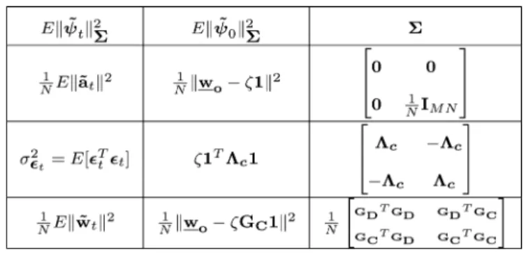
the weighting matrix we can extract information about the learning and convergence behavior of the network. In Table II, we tabulate the initial conditions (we assume the ini-tial parameter vectors are set to ) and the weighting matrices corresponding to various conventional performance measures.
Remark 5.3: In this paper, (42) provides a recursion for the
weighted deviation parameter where we assign as the final estimate instead of , which implies the CTA strategy, how-ever, the recursion also provides the performance of the ATC strategy with appropriate combination matrix and the initial condition (See Table II).
Next, we analyze the mean-square convergence performance of the single-bit diffusion approach for Gaussian regressors.
VI. SINGLE-BITDIFFUSIONWITHGAUSSIANREGRESSORS
The weighted-energy relation of (26) yields
(43)
We evaluate RHS of (43) term by term in order to find the vari-ance relation. We first partition the weighting matrix as follows: (44) Through the partitioning (44), we obtain
(45)
where we partition and such that and
. We note that the second and fourth terms in the RHS of (45) include the nonlinear function. It is not straight-forward to evaluate the expectations with this nonlin-earity, thus we introduce the following lemma.
Lemma 1: Under the Assumption 2, the Price’s theorem [5]
leads to (46) (47) where is defined as .. . . .. ...
Proof: The proof is given in Appendix A.
By (45), (46), (47), the second term on the RHS of (43) is given by
(48) where we drop the arguments of for notational sim-plicity and denotes
Similarly, the third term on the RHS of (43) is evaluated as (49) Through partitioning, the last term on the RHS of (43) yields
Corollary 1: Since and are independent from each other, similar to the Lemma 1, we obtain
(50) By the Assumption 1, the first term on the RHS of (50) yields
(51) For the last term on the RHS of (50), we introduce the following lemma.
Lemma 2: Through the Price’s theorem, we obtain
(52) where is the block diagonal matrix of such that
..
. . .. ...
with is the ’th block of and .
Proof: The proof is given in Appendix B.
As a result, by (48), (49), (50), (51) and (52), the relation (43) leads to
(53) and
where denotes
We again note that by the Assumption 1, we get which results
(54)
and define .
In the following, we resort to the vector notation, i.e., the block vectorisation operator and the block Kronecker product. Hence, the block vectorization of the weighting matrix
(54) yields
(55) Block vectorisation of the matrix is given by
. In order to denote in terms of , we
in-troduce , and . Then, we get (56) (57) By (56) and (57), we obtain (58) The -free terms in (53) are evaluated as
(59) (60)
where and .
As a result, by (55), (58), (59) and (60), the weighted-energy relation is given by
(61)
(62) (63) Iterating the weighted-energy recursion (61), (62) and (63), we obtain
.. .
TABLE III
INITIALCONDITIONS ANDWEIGHTINGMATRICES FOR THEPERFORMANCE
MEASURE OF THECONSTRUCTIONUPDATE FOR THESINGLE-BITDIFFUSION
APPROACH(FOR THESCALARDIFFUSIONAPPROACH, SET )AND THE
GLOBALMSDOF THEATC DIFFUSIONSTRATEGY FOR THESINGLE-BIT
DIFFUSIONAPPROACH(FOR THESCALARDIFFUSIONAPPROACH, SEETABLEII)
In this part of the analyzes, we do not assume that the param-eter vectors are initialized with zeros since such an assumption results in infinite terms in the matrix. Hence, we initialize with where has a small value (See Table III).
The iterations yield
(64) (65)
where and
. We note that and .
By (64) and (65), we have the following recursion
(66)
We point out that and .
Remark 6.1: The iterations of (66) require the recalculation
of for each time instants since changes with time because of (62). Evaluating the expectations, yields
..
. . .. ... (67)
where . For analytical reasons, we approximate (67) as
(68)
with and
Hence, we can calculate by iterating the following
(69)
where . In Table III, we tabulate the initial condition and the weighting matrix necessary for the recursion
iterations (69) of .
VII. STEADY-STATEANALYSIS
At the steady-state, (39) yields
In order to calculate the steady-state performance measure , we choose the weighting matrix as , then the steady-state performance measure is given by
(70) Similar to (70), the steady state mean square error for the single bit diffusion strategy is given by
(71) We point out that depends on . Once we calculate numerically by (71) or through approximations, we can ob-tain the steady state performance by (70).
VIII. TRACKINGPERFORMANCE
The diffusion implementation improves the ability of the net-work to track variations in the underlying statistical profiles [6]. In this section, we analyze the tracking performance of the com-pressive diffusion strategies in a non-stationary environment. We assume a first-order random walk model, which is com-monly used in the literature [5], for such that
where denotes a zero-mean vector process inde-pendent of the regression data and observation noise with co-variance matrix . We introduce the global
time-variant parameter vectors as and
we have the global deviation vectors as and . Then, by (26), we obtain
(72)
where with dimensions. Since
we assume that is independent from the regression data and the observation noise for all , (72) yields the following weighted-energy relation
We note that (73) is similar to (43) except for the last term . We denote matrix whose terms are 1 as
. Then, the last term in (73) is given by
where . Through (73), we get
(74) We define in (40) and (62) for scalar and single-bit diffu-sion strategies, respectively. Similarly, is introduced in (38) and (63) for the scalar (time-invariant) and single-bit diffusion strategies. We point out that (74) is different from (39) and (61) only for the term . As a result, at steady state, (70) and (74) leads
(75) Through (75) and Table II, we can obtain the tracking perfor-mance of the network for the conventional perforperfor-mance mea-sures. We point out that in the full diffusion configuration,
.
In the next section, we introduce the confidence parameter and the adaptive combination method, which provides a better trade-off in terms of the transient and the steady-state perfor-mances.
IX. CONFIDENCEPARAMETER ANDADAPTIVECOMBINATION
The cooperation among the nodes is not beneficial in general unless the cooperation rule is chosen properly [1]. For example, the uniform [22], the Metropolis [23], the relative-degree rules [8] and the adaptive combiners [25] provide improved conver-gence performance relative to the no-cooperation configuration in which nodes aim to estimate the parameter of interest without information exchange. However, the compressive dif-fusion strategies have a different difdif-fusion protocol than the full diffusion configuration. At each node , we combine the local estimates with the constructed estimates that track the local estimates of the neighboring nodes, i.e., . Es-pecially at the early stages of the adaptation, the constructed es-timates carry far less information than the local eses-timates since they are not sufficiently close to the original estimates in the mean square sense. Hence, we can consider the constructed es-timates as noisy version of the original parameter vectors. Then the overall network operation is akin to the full diffusion scheme with noisy observation. In [11], [33], [34], the authors demon-strate that for imperfect cooperation cases a node should place more weight on the local estimate in the combination step even if the node has worse quality of measurement than its neighbors. To this end, we add one more freedom of dimension to the up-date by introducing a confidence parameter . The confidence parameter determines the weight of the local estimates relative to the constructed estimates such that the new combination ma-trix is given by
(76)
where . We note that , in which case we
are confident with the local estimates, yields the no-cooperation scheme and is the full diffusion configuration where we thrust the diffused information totally.
For the new combination matrix (76), the combination of the local estimate and the constructed estimates (12) yields
(77) We note that (77) is a convex combination of the parameter vec-tors and . Hence, we can adapt the convex combi-nation weight using a stochastic gradient update [35]–[38]. Then, (77) yields
(78) In [36], authors update all combination weights ’s indirectly through a sigmoidal function. Similarly, we re-parameterize the confidence parameter using the sigmoidal function [39] and an unconstrained variable such that
(79) We train the unconstrained weight using a stochastic
gra-dient update minimizing as follows
(80) As a result, we combine the local and constructed estimates via (78), (79) and (80).
In the next section, we provide numerical examples showing the match of the theoretical derivations and simulated results, and the improved convergence performance with the adaptive confidence parameter.
X. NUMERICALEXAMPLES
In this section, we examine two distinct network scenarios where we demonstrate that the theoretical analysis accurately model the simulated results and the confidence parameter pro-vides significantly improved convergence performance. In the first example, we have a network of nodes where at each node , we observe a stationary data
for . The regression data is a zero-mean
i.i.d. Gaussian with randomly chosen standard deviation ,
i.e., where is a
uni-form random variable. The variance of the observation noise is . Hence, the signal-to-noise ratio over the network varies between 10 to 100. The standard deviation of the projec-tion operator is . The parameter of interest
is randomly chosen. Note that we examine a relatively small network with a short filter length since the computational com-plexity of the theoretical performance relations (42) and (66) in-creases exponentially with the filter length and the network size . We point out that the overall communication burden in the scalar diffusion strategy is 25% of the full dif-fusion configuration and the overall communication load in the single-bit diffusion strategy is given by 5-bits per iterations.
Fig. 4. Comparison of global MSD curves where the single-bit-1 and the scalar-1 schemes use while the single-bit-2 and the scalar-2 schemes have .
In the no-cooperation configuration, the combination matrix is given by . We use the Metropolis combination rule [23] for the full diffusion configuration where the adjacency ma-trix of the network is given by
In the Metropolis rule [24], the combination weights are chosen according to
where and denote the number of neighboring nodes for and . For the single-bit and the one-dimension diffusion strate-gies we examine the convergence performance for the
confi-dence parameter and in Fig. 4. We choose
the step sizes the same for the distributed LMS update (17) of all configurations at all nodes, i.e., . At each node, the step sizes for the construction update (18) are
(for single-bit approach) and (for one-dimension dif-fusion approach). For the single-bit difdif-fusion approach, we set to initialize . In Fig. 4, we show the global MSD curves, i.e., , of the single-bit and scalar diffusion ap-proaches and compare the performance for different values. The confidence parameter implies that we give ten times more weight to the local estimate than the constructed estimates , where . The Fig. 4 demonstrates that the confidence parameter improves the convergence performance of the compressive diffusion strategies.
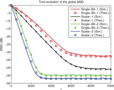
In the same example, Figs. 5 and 6 compare the convergence performance of the single-bit and the scalar diffusion strate-gies with the no-cooperation and full diffusion configurations for , which shows the match of the theoretical and
en-Fig. 5. Comparison of the global MSD and EMSE curves in the CTA strategy. (a) Global MSD curves. (b) Global EMSE curves.
Fig. 6. Comparison of the global MSD curves in the ATC diffusion strategy.
semble averaged performance results (we perform 200 indepen-dent trials). The Fig. 5 shows the time-evolution of the MSD and EMSE curves in the CTA diffusion strategy while the Fig. 6 dis-plays the time-evolution of the MSD curves in the ATC diffu-sion strategy in which the theoretical curves (42) and (66) are iterated according to the Tables II and III. We note that we ob-tain similar MSD curves in the CTA and ATC strategies since we set and the outcomes of the adaptation and combina-tion operacombina-tions contain relatively close amount of informacombina-tion.
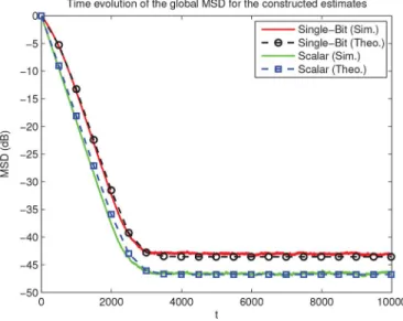
In Fig. 7, we demonstrate the convergence of the constructed estimates ’s to the parameter of interest in the mean-square sense. We point out that the recursions (42) and (66) also provide the global mean-square deviation of the constructed es-timates for the certain combination weight in Table II and the theoretical recursion matches with the simulated results.
In Fig. 8, we examine the impact of the synchronization is-sues on the estimation performance in several different sce-narios. As an example, we utilize pilot signals for the re-syn-chronization at every 10 or 100 samples. In the asynchronous events we assume that the diffused information is completely lost and each neighboring node loses the synchronization of the projection operator until the arrival of the next pilot signal, i.e., a severe synchronization event. We point out that the single-bit diffusion strategy requires the synchronization of the construc-tion updates in addiconstruc-tion to the synchronizaconstruc-tion of the projec-tion operator. Hence, the pilot signals in the single-bit diffusion
Fig. 7. The MSD curves of the construction estimate of the single-bit and scalar diffusion approaches.
Fig. 8. Impact of asynchronous events on the learning curves. (a) Single-bit diffusion strategy. (b) Scalar diffusion strategy.
scheme also re-synchronize the construction updates in each node within the neighborhood. In the Fig. 8, we observe 2 asyn-chronous events at 5001st and 6001st time instants, however, through the pilot signals at 5100th and 6100th (pilot signaling per 100 iterations) or at 5010th and 6010th (pilot signaling per 10 iterations) time instants each node can re-synchronize again. We note that single-bit diffusion strategy has performed less sensitive to the asynchronous events thanks to the relatively small learning rate of the construction update.
Fig. 9 shows the time evolution of the global MSD of the pro-posed schemes, i.e., both ensemble averaged and theoretical re-sults, in a non-stationary environment. We consider a first order
random walk model and choose in the
same configuration of the first example. In the Fig. 9, we ob-serve the match of the ensemble averaged and the theoretical results.
In Fig. 10, we compare the time evolution of the proposed schemes with the partial diffusion strategy, where each node dif-fuses only one coefficient of the parameter vector. For the pro-jection operator, we utilize a sequential selection scheme based on the round robin fashion such that
Fig. 9. Tracking performance of the proposed schemes in a non-stationary en-vironment.
Fig. 10. Comparison of the global MSD curves of the proposed schemes with the partial diffusion configuration.
Note that this scheme satisfies the constraint to span the whole parameter space. Correspondingly, we use a sequential partial-diffusion scheme such that each node shares the same coeffi-cients in order. In the proposed schemes, we choose and the step sizes of the all schemes are . For the
con-struction updates, and in the single-bit
and scalar diffusion strategies, respectively. The Fig. 10 shows that sequential selection scheme provides enhanced estimation performance also for the compressive diffusion strategies. In the Fig. 10, we also observe that both scalar diffusion and partial diffusion approaches achieve comparable performance.
We can enhance the performance of the scheme through the adaptation of the confidence parameter irrespective of the cooperation rule. As an example, in Fig. 11, we compare the time evolution of the MSD of the scalar diffusion scheme for the adaptive and fixed confidence parameter cases with the Metropolis and uniform combination rules. We use the same configuration with the example 1, initialize , and set . Additionally, in Fig. 12, we also plot the time-evo-lution of the scalar diffusion scheme for . Note that the
Fig. 11. Comparison of the adaptive and fixed confidence parameter for the Metropolis and uniform combination rules.
Fig. 12. Comparison of the adaptive and fixed confidence parameter for the scalar diffusion scheme.
adaptive scheme converges as fast as scheme while achieving smaller steady-state error similar to scheme. Hence, through the confidence parameter we can enhance the performance of the compressive diffusion scheme for certain scenarios.
In the second example, we examine the convergence per-formance of the adaptive confidence parameter in a relatively
large network with a long filter length .
We again observe a stationary data for
. The regressor data is zero-mean i.i.d. Gaussian whose standard deviation is around 0.4. The observa-tion noise is zero-mean i.i.d. Gaussian whose variance is . We note that the signal-to-noise ratio is around 1.55 over the network, which is relatively lower than the signal-to-noise ratio for the example 1. The variance of the
projection operator is for the
scalar (single-bit) diffusion scheme. The parameter of interest is randomly chosen from a Gaussian distribution and normalized such that . We point out that in this
Fig. 13. The global MSD curves in relatively large network and long filter length while the confidence parameter is adapted in time.
example, the overall communication burden in the scalar diffu-sion strategy is 1% of the full diffudiffu-sion configuration while the overall communication load in the single-bit diffusion strategy is given by 20-bits per iterations.
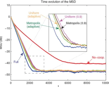
We again use the Metropolis rule as the combination rule, however, in this example, we adapt the confidence parameter through (79) and (80) where we resort to the convex mixture of the adaptive filtering algorithms [35]–[38]. We also choose the step sizes the same for the distributed LMS update (17) of all configurations at all nodes, i.e., . In example 2, the step sizes for the construction update (18) are (for the single-bit diffusion approach) and (for the scalar diffu-sion approach). We set in (80). The Fig. 13 shows the global MSD curves of the no-cooperation, single-bit, scalar and full diffusion strategies. We observe that the adaptive confi-dence parameter improves the convergence performance of the compressive diffusion strategies far more such that they achieve comparable performance while the reduction of the communi-cation load is tremendous.
XI. CONCLUSION
In the diffusion based distributed estimation strategies, the communication load increases far more in the large networks or highly connected network of nodes. Hence, the compressive diffusion approach plays an essential role in achieving compa-rable convergence performance to the full diffusion configura-tions while reducing the communication load tremendously. We provide a complete performance analysis for the compressive diffusion strategies. We analyze the mean-square convergence, the steady-state behavior and the tracking performance of the scalar and single-bit diffusion approaches. The numerical ex-amples show that the theoretical analysis model the simulated results accurately. Additionally, we introduce the confidence pa-rameter concept, which adds one more freedom of dimension to the combination rule in order to improve the convergence per-formance. When we adapt the confidence parameter using the well-known adaptive mixture algorithms, we observe enormous enhancement in the convergence performance of the compres-sive diffusion strategies even for relatively long filter lengths.
APPENDIXA
PROOFFORLEMMA1
We first show the equality of (46) for the two-node case. Then the extension for a larger network is straight forward. We can rewrite the term on the left hand side (LHS) of (46) as
(81)
After some algebra, (81) yields
(82) In order to evaluate the expectations on the RHS of (82), by the Assumption 2 and the Price’s result [40]–[42], we obtain
(83) Rearranging (83) into a matrix product form leads (46). Following the same way, we can also get (47) and the proof is concluded.
APPENDIXB PROOF FORLEMMA2
We derive the RHS of (52) for the two-node case for nota-tional simplicity, however, the derivation holds for any order of network. For the two-node case, the LHS of (52) yields
We re-emphasize that the regressor is spatially and tem-porarily independent. Hence, we obtain
(84)
Using the Price’s result, we can evaluate the last two terms on
the RHS of (84) for as
We point out that the terms involving the diagonal entries of the weighting matrix in (84) do not include the deviation terms. As a result, rearranging (84) into a compact form results in (52). This concludes the proof.
REFERENCES
[1] A. H. Sayed, S.-Y. Tu, J. Chen, X. Zhao, and Z. J. Towfic, “Diffusion strategies for adaptation and learning over networks: An examination of distributed strategies and network behavior,” IEEE Signal Process.
Mag., vol. 30, no. 3, pp. 155–171, 2013.
[2] D. Li, K. D. Wong, Y. H. Hu, and A. M. Sayeed, “Detection, classi-fication, and tracking of targets,” IEEE Signal Process. Mag., vol. 19, no. 2, pp. 17–29, 2002.
[3] I. Akyildiz, W. Su, Y. Sankarasubramaniam, and E. Cayirci, “A survey on sensor networks,” IEEE Commun. Mag., vol. 40, no. 8, pp. 102–114, 2002.
[4] D. Estrin, L. Girod, G. Pottie, and M. Srivastava, “Instrumenting the world with wireless sensor networks,” in Proc. Int. Conf. Acoust.,
Speech, Signal Process. (ICASSP), 2001, vol. 4, pp. 2033–2036, vol. 4.
[5] A. H. Sayed, Fundamentals of Adaptive Filtering. New York, NY, USA: Wiley, 2003.
[6] C. G. Lopes and A. H. Sayed, “Diffusion least-mean squares over adap-tive networks: Formulation and performance analysis,” IEEE Trans.
Signal Process., vol. 56, no. 7, pp. 3122–3136, 2008.
[7] F. S. Cattivelli and A. H. Sayed, “Diffusion LMS strategies for dis-tributed estimation,” IEEE Trans. Signal Process., vol. 58, no. 3, pp. 1035–1048, 2010.
[8] F. S. Cattivelli, C. G. Lopes, and A. H. Sayed, “Diffusion recursive least-squares for distributed estimation over adaptive networks,” IEEE
Trans. Signal Process., vol. 56, no. 5, pp. 1865–1877, 2008.
[9] F. S. Cattivelli and A. H. Sayed, “Diffusion strategies for distributed Kalman filtering and smoothing,” IEEE Trans. Autom. Control, vol. 55, no. 9, pp. 2069–2084, 2010.
[10] S.-Y. Tu and A. H. Sayed, “Diffusion strategies outperform consensus strategies for distributed estimation over adaptive networks,” IEEE
Trans. Signal Process., vol. 60, no. 12, pp. 6217–6234, 2012.
[11] X. Zhao, S.-Y. Tu, and A. H. Sayed, “Diffusion adaptation over networks under imperfect information exchange and non-stationary data,” IEEE Trans. Signal Process., vol. 60, no. 7, pp. 3460–3475, 2012.
[12] M. O. Sayin and S. S. Kozat, “Single bit and reduced dimension diffu-sion strategies over distributed networks,” IEEE Signal Process. Lett., vol. 20, no. 10, pp. 976–979, 2013.
[13] D. L. Donoho, “Compressed sensing,” IEEE Trans. Inf. Theory, vol. 52, no. 4, pp. 1289–1306, 2006.
[14] R. G. Baraniuk, V. Cevher, and M. B. Wakin, “Low-dimensional models for dimensionality reduction and signal recovery: A geometric perspective,” Proc. IEEE, vol. 98, no. 6, pp. 959–971, 2010. [15] R. Arablouei, S. Werne, and K. Dogancay, “Partial-diffusion recursive
least-squares estimation over adaptive networks,” in Proc. IEEE
5th Int. Workshop on Computat. Adv. Multi-Sens. Adapt. Process. (CAMSAP), 2013, pp. 89–92.
[16] R. Arablouei, S. Werner, Y. F. Huang, and K. Dogancay, “Distributed least mean square estimation with partial diffusion,” IEEE Trans.
Signal Process., vol. 62, no. 2, pp. 472–483, 2014.
[17] R. Arablouei, S. Werner, Y. F. Huang, and K. Dogancay, “Adaptive distributed estimation based on recursive least-square and partial dif-fusion,” IEEE Trans. Signal Process., vol. 62, no. 14, pp. 3510–3522, 2014.
[18] S. Chouvardas, K. Slavakis, and S. Theodoridis, “Trading off com-plexity with communication costs in distributed adaptive learning via Krylov subspaces for dimensionality reduction,” IEEE J. Sel. Topics
Signal Process., vol. 7, no. 2, pp. 257–273, 2013.
[19] S. Xie and H. Li, “Distributed LMS estimation over networks with quantised communications,” Int. J. Contr., vol. 86, no. 3, pp. 478–492, 2013.
[20] A. Ribeiro, G. B. Giannakis, and S. I. Roumeliotis, “SOI-KF: Dis-tributed Kalman filtering with low-cost communications using the sign of innovations,” IEEE Trans. Signal Process., vol. 54, no. 12, pp. 4782–4795, 2006.
[21] H. Sayyadi and M. R. Doostmohammadian, “Finite-time consensus in directed switching network topologies and time-delayed communica-tions,” Scientia Iranica, vol. 18, no. 1, pp. 75–85, Feb. 2011. [22] V. D. Blondel, J. M. Hendrickx, A. Olshevsky, and J. N. Tsitsiklis,
“Convergence in multiagent coordination, consensus and flocking,” in
Proc. Joint 44th IEEE Conf. Decision Contr. Eur. Contr. Conf. (CDC-ECC), Seville, Spain, Dec. 2005, pp. 2996–3000.
[23] L. Xiao and S. Boyd, “Fast linear iterations for distributed averaging,”
Syst. Contr. Lett., vol. 53, no. 1, pp. 65–78, 2004.
[24] N. Metropolis, A. W. Rosenbluth, M. N. Rosenbluth, A. H. Teller, and E. Teller, “Equation of state calculations by fast computing machines,”
J. Chem. Phys. vol. 21, no. 6, pp. 1087–1092, 1953 [Online].
Avail-able: http://scitation.aip.org/content/aip/journal/jcp/21/6/10.1063/1. 1699114
[25] N. Takahashi, I. Yamada, and A. H. Sayed, “Diffusion least-mean squares with adaptive combiners: Formulation and performance anal-ysis,” IEEE Trans. Signal Process., vol. 58, no. 9, pp. 4795–4810, 2010. [26] E. Barker and J. Kelsey, “Recommendation for random number generation using deterministic random bit generators,” in NIST
SP800-90A, 2012 [Online]. Available:
http://csrc.nist.gov/publica-tions/nistpubs/800-90A/SP800-90A.pdf
[27] J. Joutsensalo and T. Ristaniemi, “Synchronization by pilot signal,” in
Proc. Int. Conf. Acoust., Speech, Signal Process. (ICASSP), 1999, pp.
2663–2666.
[28] F. T. Castoldi and M. L. R. Campos, “Application of a minimum-distur-bance description to constrained adaptive filters,” IEEE Signal Process.
Lett., vol. 20, no. 12, pp. 1215–1218, 2013.
[29] M. A. Donmez, H. A. Inan, and S. S. Kozat, “Adaptive mixture methods based on Bregman divergences,” Digit. Signal Process., vol. 23, pp. 86–97, 2013.
[30] A. H. Sayed, T. Y. Al-Naffouri, and V. H. Nascimento, “Energy con-servation in adaptive filtering,” in Nonlinear Signal and Image
Pro-cessing: Theory, Methods, and Applications, K. E. Barner and G. R.
Arce, Eds. Boca Raton, FL, USA: CRC, 2003.
[31] T. Y. Al-Naffouri and A. H. Sayed, “Transient analysis of adaptive filters with error nonlinearities,” IEEE Trans. Signal Process., vol. 51, no. 3, pp. 653–663, 2003.
[32] T. Y. Al-Naffouri and A. H. Sayed, “Transient analysis of data-normal-ized adaptive filters,” IEEE Trans. Signal Process., vol. 51, no. 3, pp. 639–652, 2003.
[33] X. Zhao and A. H. Sayed, “Combination weights for diffusion strate-gies with imperfect information exchange,” in Proc. IEEE Int. Conf.
Commun., 2012, pp. 398–402.
[34] S.-Y. Tu and A. H. Sayed, “Adaptive networks with noisy links,” in
Proc. IEEE Global Telecommun. Conf., 2011, pp. 1–5.
[35] J. Arenas-Garcia, V. Gomez-Verdejo, and A. R. Figueiras-Vidal, “New algorithms for improved adaptive convex combination of LMS transversal filters,” IEEE Trans. Instrum. Meas., vol. 54, no. 6, pp. 2239–2249, 2005.
[36] J. Arenas-Garcia, A. R. Figueiras-Vidal, and A. H. Sayed, “Mean-square performance of a convex combination of two adaptive filters,” IEEE
Trans. Signal Process., vol. 54, no. 3, pp. 1078–1090, 2006.
[37] M. T. M. Silva and V. H. Nascimento, “Improving the tracking capa-bility of adaptive filters via convex combination,” IEEE Trans. Signal
Process., vol. 56, no. 7, pp. 3137–3149, 2008.
[38] S. S. Kozat, A. T. Erdogan, A. C. Singer, and A. H. Sayed, “Steady state MSE performance analysis of mixture approaches to adaptive fil-tering,” IEEE Trans. Signal Process., vol. 58, no. 8, pp. 4050–4063, Aug. 2010.
[39] J. Han and C. Moraga, “The influence of the sigmoid function param-eters on the speed of back propagation learning,” in From Natural to
Artificial Neural Computation, J. Mira and F. Sandoval, Eds. Berlin
Heidelberg: Springer, 1995.
[40] R. Price, “A useful theorem for nonlinear devices having gaussian in-puts,” IEEE Trans. Inf. Theory, vol. 4, no. 2, pp. 69–72, 1958. [41] E. McMahon, “An extension of price’s theorem (corresp.),” IEEE
Trans. Inf. Theory, vol. 10, no. 2, pp. 168–168, 1964.
[42] T. Koh and E. J. Powers, “Efficient methods of estimate correlation functions of Gaussian processes and their performance analysis,” IEEE
Trans. Acoust., Speech, Signal Process., vol. 33, no. 4, pp. 1032–1035,
1985.
Muhammed O. Sayin was born in Erzincan, Turkey, in 1990. He received the B.S. degree with high honors in electrical and electronics engineering from Bilkent University, Ankara, Turkey, in 2013.
He is currently working toward the M.S. degree in the Department of Electrical and Electronics Engineering at Bilkent University. His research interests include distributed signal processing, adap-tive filtering theory, machine learning, and statistical signal processing.
Suleyman Serdar Kozat (A’10–M’11–SM’11) re-ceived the B.S. degree with full scholarship and high honors from Bilkent University, Turkey. He received the M.S. and Ph.D. degrees in electrical and com-puter engineering from University of Illinois at Ur-bana Champaign, UrUr-bana. He is a graduate of Ankara Fen Lisesi.
After graduation, he joined IBM Research, T. J. Watson Research Lab, Yorktown, New York, as a Re-search Staff Member in the Pervasive Speech Tech-nologies Group. While doing his Ph.D., he was also working as a Research Associate at Microsoft Research, Redmond, WA, in the Cryptography and Anti-Piracy Group. He holds several patent inventions due to his research accomplishments at IBM Research and Microsoft Research. After serving as an Assistant Professor at Koc University, he is currently an Assistant Professor (with the Associate Professor degree) at the electrical and electronics department of Bilkent University.
Dr. Kozat is President of the IEEE Signal Processing Society, Turkey Chapter. He has been elected to the IEEE Signal Processing Theory and Methods Tech-nical Committee and IEEE Machine Learning for Signal Processing TechTech-nical Committee, 2013. He has been awarded IBM Faculty Award by IBM Research in 2011, Outstanding Faculty Award by Koc University in 2011 (granted the first time in 16 years), Outstanding Young Researcher Award by the Turkish National Academy of Sciences in 2010, ODTU Prof. Dr. Mustafa N. Parlar Re-search Encouragement Award in 2011, Outstanding Faculty Award by Bilim Kahramanlari, 2013 and holds Career Award by the Scientific Research Council of Turkey, 2009.