Development of a modular control algorithm for high precision positioning systems

DEVELOPMENT OF A MODULAR

CONTROL ALGORITHM FOR HIGH

PRECISION POSITIONING SYSTEMS

a thesis

submitted to the department of mechanical

engineering

and the graduate school of engineering and science

of bilkent university

in partial fulfillment of the requirements

for the degree of

master of science

By

Nurcan Ge¸cer Ulu

August, 2012

I certify that I have read this thesis and that in my opinion it is fully adequate, in scope and in quality, as a thesis for the degree of Master of Science.

Assist. Prof. Dr. Melih C¸ akmakcı (Advisor)

I certify that I have read this thesis and that in my opinion it is fully adequate, in scope and in quality, as a thesis for the degree of Master of Science.

Assist. Prof. Dr. Yi˘git Karpat

I certify that I have read this thesis and that in my opinion it is fully adequate, in scope and in quality, as a thesis for the degree of Master of Science.

Prof. Dr. Hitay ¨Ozbay

Approved for the Graduate School of Engineering and Science:

Prof. Dr. Levent Onural Director of the Graduate School

ABSTRACT

DEVELOPMENT OF A MODULAR CONTROL

ALGORITHM FOR HIGH PRECISION POSITIONING

SYSTEMS

Nurcan Ge¸cer Ulu

M.S. in Mechanical Engineering

Supervisor: Assist. Prof. Dr. Melih C¸ akmakcı August, 2012

In the last decade, micro/nano-technology has been improved significantly. Micro/nano-technology related products started to be used in consumer mar-ket in addition to their applications in the science and technology world. These developments resulted in a growing interest for high precision positioning systems since precision positioning is crucial for micro/nano-technology related applica-tions. With the rise of more complex and advanced applications requiring smaller parts and higher precision performance, demand for new control techniques that can meet these expectations is increased.

The goal of this work is developing a new control technique that can meet increased expectations of precision positioning systems. For this purpose, control of a modular axis positioning system is studied in this thesis. The multi-axis precision positioning system is constructed by assembling modular single-multi-axis stages. Therefore, a single-axis stage can be used in several configurations. Model parameters of a single-axis stage change depending on which axis it is used for. For this purpose, an iterative learning controller is designed to improve tracking performance of a modular single-axis stage to help modular sliders adapting to repeated disturbances and nonlinearities of the axis they are used for. When modular single-axis stages are assembled to form multi-axis systems, the interac-tion between the axes should be considered to operate stages simultaneously. In order to compensate for these interactions, a multi input multi output (MIMO) controller can be used such as cross-coupled controller (CCC). Cross-coupled con-troller examines the effects between axes by controlling the contour error resulting in an improved contour tracking.

iv

In this thesis, a controller featuring cross-coupled control and iterative learning control schemes is presented to improve contour and tracking accuracy at the same time. Instead of using the standard contour estimation technique proposed with the variable gain cross-coupled control, presented control design incorporates a computationally efficient contour estimation technique. In addition to that, implemented contour estimation technique makes the presented control scheme more suitable for arbitrary nonlinear contours and multi-axis systems. Also, using the zero-phase filtering based iterative learning control results in a practical design and an increased applicability to modular systems. Stability and convergence of the proposed controller has been shown with the necessary theoretical analysis. Effectiveness of the control design is verified with simulations and experiments on two-axis and three-axis positioning systems. The resulting controller is shown to achieve nanometer level contouring and tracking performance.

Keywords: Iterative learning control, cross-coupled control, precision motion con-trol.

¨

OZET

Y ¨

UKSEK HASSAS˙IYETL˙I POZ˙ISYONLAMA

S˙ISTEMLER˙I ˙IC

¸ ˙IN MOD ¨

ULER KONTROL

ALGOR˙ITMASI GEL˙IS

¸T˙IR˙ILMES˙I

Nurcan Ge¸cer Ulu

Makine M¨uhendisli˘gi, Y¨uksek Lisans Tez Y¨oneticisi: Assist. Prof. Dr. Melih C¸ akmakcı

A˘gustos, 2012

Son on yıl i¸cinde, mikro/nano-teknoloji b¨uy¨uk ¨ol¸c¨ude geli¸sti. Mikro/nano-teknoloji ile ilgili ¨ur¨unler bilim ve teknoloji d¨unyasındaki uygulamaların yani sira t¨uketici marketinde de yer almaya ba¸sladı. Bu geli¸smeler y¨uksek hassasiyetli pozisyonlama sistemlerine olan ilgiyi arttırdı ¸c¨unk¨u y¨uksek hassasiyetli pozisyon-lama sistemleri mikro/nano-teknoloji ile ilgili uygupozisyon-lamalarda cok ¨onemli bi yere sahiptir. Daha kompleks ve ileri d¨uzeydeki uygulamalarin daha sıkı toleranslar ve daha k¨u¸c¨uk parcalar gerektirmesi sonucunda bu beklentileri kar¸sılayabilecek yeni kontrol tekniklerine olan ilgi artmı¸stır.

Bu ¸calı¸smanın amacı y¨uksek hassasiyetli pozisyonlama sistemlerine y¨onelik artan ilgiyi kar¸sılayabilecek yeni bir kontrol tekni˘gi geli¸stirmektir. Bu ama¸cla, mod¨uler ¸cok eksenli pozisyonlama sisteminin kontrol¨u ¸calısılmı¸stır. Bahsi ge¸cen ¸cok eksenli pozisyonlama sistemi mod¨uler tek eksenli kızakların birle¸stirilmesiyle olu¸sturulmu¸stur. B¨oylece, tek eksenli pozisyonlama sistemi birka¸c ¸sekilde kul-lanılır ve kullanıldı˘gı alana g¨ore model parametreleri de˘gi¸sir. Bu sebeple, mod¨uler kızakların kullanıldı˘gı alana uyum sa˘glamaları ve takip hatalarını azaltabilmeleri i¸cin tekrarlamalı ¨o˘grenme kontrolc¨us¨u geli¸stirilmi¸stir. C¸ ok eksenli pozisyonlama sisteminde, kızaklar aynı anda hareket ettirildi˘ginde birbirleri arasındaki etk-ile¸simler g¨oz ¨on¨unde bulundurulmalıdır. Bu etkile¸simlerin etkisini azaltmak i¸cin ¸capraz ba˘gla¸sımlı kontrolc¨u kullanılabilir ve b¨oylece kontur hatası azaltılabilir.

Bu tezde, takip ve kontur hatasını birlikte azaltmak ¨uzere ¸capraz ba˘gla¸sımlı kontrolc¨u ve tekrarlamalı ¨o˘grenme kontrolc¨us¨un¨un bir arada kullanıldı˘gı bir kon-trolc¨u geli¸stirilmi¸stir. C¸ apraz ba˘gla¸sımlı kontrolc¨u ile birlikte sunulan kontur tahmin y¨ontemi yerine i¸slemsel olarak daha verimli bir kontur tahmin y¨ontemi kullanılmı¸stır. Bunun yanında, kullanılan y¨ontem herhangi bir kontur kontrol¨u

vi

i¸cin ve ¸cok eksenli sistemlerde kullanmak i¸cin daha uygundur. Ayrıca, tekrar-lamalı ¨o˘grenme kontrolc¨us¨un¨un kullanılması, pratik bir tasarima ve mod¨uler sistemlere uygunlu˘g arttırmaya yarar. Ayrıca, ¨onerilen kontrolc¨un¨un kararlılık ve yakınsama karakteristi˘gi incelenmi¸stir. Kontrolc¨un¨un etkilili˘gi iki ve ¨u¸c ek-senli sistem ¨uzerinde yapılan simulasyon ve deneylerle g¨osterilmi¸stir. Sonu¸cta ortaya ¸cıkan kontrolc¨u ile nanometre hassasiyetinde takip ve kontur performansı g¨ozlemlenmi¸stir.

Anahtar s¨ozc¨ukler : Tekrarlamalı ¨o˘grenme kontrol¨u, ¸capraz ba˘gla¸sımlı kontrol, hassas haraket kontrol¨u.

Acknowledgement

I would like to express my sincere gratitude to my advisor, Assist. Prof. Melih C¸ akmak¸cı, for his encouragement, guidance and support throughout my thesis work. His perpetual energy as an advisor and enthusiasm in research had motivated me and made the research period smooth and rewarding.

I would also like to thank all members of Bilkent University Mechanical En-gineering Department. Especially, I would like to thank department chair, Prof. Adnan Akay for his support. Moreover, I owe special thanks to Assist. Prof. Sinan Filiz for sharing his experience in precision positioning systems. His help was very important throughout this research. I would also like to express my thanks to S¸akir Baytaro˘glu for his helpful advice and comments. I would also like to thank undergraduate students working in our lab, Ersun Sozen and Oytun Ugurel.

I would also like to thank my family and friends for their support, love and encouragement.

I also wish to thank The Scientific and Technology Reserch Council of Turkey (T ¨UB˙ITAK) for the support of this research through 1001 grant. Moreover, Na-tional Scholarship for Master of Science Students provided by T ¨UB˙ITAK (2210-Yurt ˙I¸ci Y¨uksek Lisans Bursu) is gratefully acknowledged.

Above all, I would like to present my deepest thanks to my husband, Erva Ulu.

Contents

1 Introduction 1

2 System Setup and Modeling 4

2.1 System Setup . . . 4

2.1.1 Modular Single-Axis Slider System . . . 5

2.1.2 Control Setup and Testbed . . . 5

2.1.3 Multi-Axis Positioning System . . . 6

2.2 Modeling . . . 7

2.2.1 Mathematical Model of The Modular Single-Axis Slider System . . . 7

2.2.2 Model Improvement Tests . . . 11

3 Literature Survey 16 3.1 Tracking Control . . . 17

3.2 Contouring Control . . . 19

CONTENTS ix

3.2.2 Variations and Combinations of CCC . . . 21

3.2.3 Contour Error Estimation Models . . . 22

3.2.4 Model Predictive Contouring Control . . . 25

3.3 Conclusion . . . 26

4 Development of The Control Algorithm 27 4.1 Iterative Learning Controller via Zero-phase Filtering . . . 29

4.2 Cross-coupled Control with Contouring Error Vector Approach . . 30

4.3 Learning Based Cross-coupled Controller . . . 32

4.4 Stability and Convergence . . . 33

5 Simulation and Experiment 39 5.1 Trajectory Planning . . . 39

5.2 Single-axis Slider System . . . 41

5.2.1 Simulation Results . . . 41

5.2.2 Experimental Results . . . 42

5.3 Two-axis Slider System . . . 43

5.3.1 Simulation Results . . . 43

5.3.2 Experimental Results . . . 45

5.4 Three-axis Slider System . . . 47

5.4.1 Simulation Results . . . 48

CONTENTS x

6 Robustness 52

6.1 Predicted Uncertainties and Disturbances of the System . . . 52

6.2 Test Setup . . . 54

6.3 Test Results . . . 55

6.3.1 Sliding Mass Increase Test . . . 55

6.3.2 Constant Axial Forces Test . . . 56

6.3.3 Sudden Axial Force Test . . . 58

6.4 Conclusion . . . 59

7 Conclusion and Future Work 62

A Simulink Diagrams 71

B Labview Implementations 74

List of Figures

2.1 Single-axis slider system . . . 5

2.2 Closed loop control setup of the single-axis system . . . 6

2.3 Photograph of testbed for the single-axis slider system . . . 7

2.4 Two-axis positioning system . . . 8

2.5 Three-axis positioning system . . . 8

2.6 Forces acting on the moving slider . . . 9

2.7 Free body diagram of the moving slider . . . 10

2.8 Dynamic model of the single-axis system . . . 10

2.9 Block diagram of the mathematical model . . . 11

2.10 Velocity step response . . . 13

2.11 Step response characteristics comparison for (a) Position, (b) Po-sition Error and (c) Controller Output . . . 14

3.1 Trajectory tracking . . . 17

3.2 Tracking and contour error . . . 19

LIST OF FIGURES xii

3.4 Block Diagram of Position Based CCC . . . 22

3.5 Geometrical Relations of Contour Error (adopted from[1]) . . . . 24

3.6 Model Predictive Contouring Control Diagram [2] . . . 25

4.1 Block Diagram of ILC via Zero-Phase Filtering with Feedback Con-troller [3] . . . 28

4.2 Reorganized Block Diagram of ILC via Zero-Phase Filtering with Feedback Controller . . . 29

4.3 Block Diagram of Cross-coupled Control with Contouring Error Vector Approach . . . 30

4.4 2D contour with its tangents and normals . . . 31

4.5 Learning Based Cross-coupled Controller for Two-axis Systems . . 32

4.6 Learning Based Cross-coupled Controller for Multi-axis Systems . 33 4.7 Block Diagram of Uncoupled System . . . 33

4.8 Block Diagram of Coupled System . . . 35

4.9 Block Diagram of Equivalent Control System . . . 36

4.10 RMS Contour Error for (a) Simulation and (b) Experiment . . . 38

5.1 A Pulse Shaped Jerk Profile and Its First, Second and Third Inte-grals as Acceleration, Velocity and Position Profiles . . . 40

5.2 Single-axis System Simulation - Position Tracking . . . 41

5.3 Single-axis System Simulation- Position Error . . . 42

LIST OF FIGURES xiii

5.5 Single-axis System Experiment- Position Error . . . 43

5.6 Two-axis System Simulation - RMS Error Values for The Nonlinear Contour . . . 44

5.7 Two-axis System Simulation for The Nonlinear Contour . . . 45

5.8 Experimental Results of Two-axis System for The Nonlinear Contour 46

5.9 Two-axis System Experiment - RMS Error Values for The Nonlin-ear Contour . . . 47

5.10 Three-axis System Simulation for The Nonlinear Contour . . . 48

5.11 Three-axis System Simulation - RMS Error Values for The Non-linear Contour . . . 49

5.12 Three-axis System Experiments - RMS Error Values for The Non-linear Contour . . . 50

5.13 (a) x-y Plane, (b) y-z Plane, (c) x-z Plane and (d) 3 Dimensional Experimental Results of Three-axis System for The Nonlinear Con-tour . . . 51

6.1 Robustness Test Setup . . . 54

6.2 System Response with 0.1N Sudden Axial Force for Horizontal Axis 58

6.3 System Response with 0.1N Sudden Axial Force for Vertical Axis 59

A.1 Simulink Block Diagram for ILC . . . 71

A.2 Simulink Block Diagram for Learning Based Cross Coupled Con-trol in Two-axis . . . 72

A.3 Simulink Block Diagram for Learning Based Cross Coupled Con-trol in Three-axis . . . 73

LIST OF FIGURES xiv

B.1 Front Panel for Single-axis ILC Control . . . 74

B.2 Labview VI for Single-axis ILC Control . . . 75

B.3 Front Panel for Two-axis Learning Based Cross-coupled Control . 76

B.4 Labview VI for Two-axis Learning Based Cross-coupled Control . 77

B.5 Front Panel for Three-axis Learning Based Cross-coupled Control 78

B.6 Labview VI for Three-axis Learning Based Cross-coupled Control 79

C.1 Trajectory for single-axis simulations and experiments . . . 80

C.2 (a) x-axis trajectory, (b) y-axis trajectory and (c) contour for the two-axis simulation and experiments . . . 81

C.3 (a) x-axis trajectory, (b) y-axis trajectory, (c) z-axis trajectory and (d) contour for the three-axis simulation and experiments . . . 82

List of Tables

4.1 Parameters . . . 34

5.1 Two-axis System simulation - RMS error values for the nonlinear contour . . . 44

5.2 Two-axis System experiments - RMS error values for the nonlinear contour . . . 47

5.3 Three-axis system simulation - RMS error values for the nonlinear contour . . . 49

5.4 Three-axis system experiment - RMS error values for the nonlinear contour . . . 50

6.1 Sliding Mass Inrease Test Results for 1st Run . . . 55

6.2 Sliding Mass Inrease Test Results for 20th Run . . . 55

6.3 Constant Axial Force Test in x-axis for 1st _{Run (two-axis system) 56}

6.4 Constant Axial Force Test in x-axis for 20th _{Run (two-axis system) 56}

6.5 Constant Axial Force Test in y-axis for 1st _{Run (two-axis system) 56}

LIST OF TABLES xvi

6.7 Constant Axial Force Test in both x and y axes for 1st _Run

(two-axis system) . . . 57

6.8 Constant Axial Force Test in both x and y axes for 20th _Run

(two-axis system) . . . 58

6.9 Constant Axial Force Test in z axis for 1st _{Run (three-axis system) 59}

6.10 Constant Axial Force Test in z axis for 20st Run (three-axis system) 60

6.11 Constant Axial Force Test in all x-y-z axes for 1st Run (three-axis system) . . . 60

6.12 Constant Axial Force Test in all x-y-z axes for 20st _{Run (three-axis}

Chapter 1

Introduction

Recently, micro/nano-technology has been improved significantly. Micro/nano-technology related products started to be used in consumer market in addition to their applications in the science and technology world. These developments re-sulted in a growing interest for high precision positioning systems since precision positioning is crucial for micro/nano-technology related applications. For exam-ple, multi-axis precision positioning is required in micro/nano-scale manufactur-ing and assembly, optical component alignment systems, scannmanufactur-ing microscopy applications, nano-particle placement applications, cell/tissue engineering and etc.[4, 5, 6]. With the rise of more complex and advanced applications requiring smaller parts and higher precision performance, demand for new control tech-niques that can meet these expectations is increased.

In an effort to develop a new control technique for high precision positioning systems, control of a modular positioning system is studied in this thesis. The positioning system is modular in the sense that it is constructed by the same single-axis slider to form two-axis and three-axis slider systems. Here, it is aimed to be able to control single-axis, two-axis and three-axis precision positioning sys-tems. In a single-axis precision positioning system, tracking performance is one of the most important factors. For multi-axis systems, high contouring perfor-mance is also required. Therefore, in order to achieve high precision positioning, tracking and contouring performance should be considered.

In literature, most of the studies on contour control focus on increasing track-ing performance of each axis in order to lead better contour performance. More-over, some specially designed multi-input-multi-output (MIMO) control algo-rithms consider the effects between moving axes so that the resulting contour performance is improved. Tracking control algorithms and contour control al-gorithms can also be used together to achieve higher tracking and contouring performances.

In this thesis, an new method based on cross-coupled control (CCC) and iterative learning control (ILC) which benefits from the contouring error vector approach is presented for multi-axis systems. CCC is a special type of MIMO control that uses contour error as the control parameter whereas ILC is a feed-forward control method that is widely used for tracking control. Since proposed method also benefits from the contouring error estimation vector approach, it is computationally more efficient, more suitable for coupling gain calculations of arbitrary nonlinear contours and easier to implement on multi-axis systems than traditional approaches. Moreover, the presented method utilizes ILC via zero-phase filtering so that the design process for ILC is practical and suitable for modular systems. Since the positioning system is modular, the single-axis stage can be used as x-axis, y-axis or z-axis. Use of iterative learning control also helps modular sliders adapting to repeated disturbances and nonlinearities of the axis they are used for.

Positioning systems, with the increased demand from the industry, are re-quired to have both high precision and high speed operation capabilities in recent years. However, uncontrolled accelerating or decelerating motion causes residual vibrations during high-speed operation. Hence, the accuracy of the system de-creases whereas the settling time inde-creases. However, residual vibrations can be prevented by planning the reference trajectory of the system in a way that accel-eration and decelaccel-eration phases are smoothed out. Although control algorithm presented in this thesis increases contouring and tracking performance, reference trajectory planning is essential for further improvements to achieve high preci-sion. For this purpose, generic s-curve method is employed in this thesis. In this method, position input is designed as an s-shaped curve so that there is no

sudden change in acceleration and velocity during the operation.

The remainder of this thesis is organized as follows. Chapter 2 introduces the modular positioning system used in this thesis with its control setup. Also, the single-axis slider system is examined through its mathematical model considering the assembly configurations. In Chapter 3, tracking control and contour control approaches used in literature are discussed. Chapter 4 presents the learning based cross-coupled controller as well as the cross-coupled controller and iterative learning controller. Stability and convergence of the controller is also analyzed in this section. Effectiveness of the presented control design is verified with simulations and experiments on two-axis and three-axis positioning systems using nonlinear contours in Chapter 5. Simulation and experiment results are supplied for single-axis system control for an s-curved trajectory. Trajectory planning procedure is also explained in this chapter. In Chapter 6, robustness of the control algorithm implementation is tested through some experiments that are designed considering the expected disturbances and system uncertainties. Conclusion and future work is discussed in Chapter 7.

Chapter 2

System Setup and Modeling

This chapter introduces the positioning system used in this thesis with its control setup. Also, the single-axis slider system is examined through its mathematical model development. For this purpose, first, components of the single-axis slider system are explained. Then, control setup is described with the electronic equip-ment and software used for the control impleequip-mentation. Whole system with the physical environment is also given as the testbed. Multi-axis configurations of the slider system that are used for the experiments are also provided. To design a controller, mathematical model is an essential requirement. For this reason, a theoretical model of the single-axis slider system is derived and improved by experiments. This section is a revised version of the work given in [7]

2.1

System Setup

Control of single-axis, two-axis and three-axis positioning system is practiced in this thesis. Therefore, system setup includes single-axis and multi-axis (two-axis and three-(two-axis) positioning systems. Moreover, there are other electronicl components and software used for the control of these positioning systems. In order to explain the system setup, single-axis slider system, control setup and multi-axis positioning system are described in this section.

Figure 2.1: Single-axis slider system

2.1.1

Modular Single-Axis Slider System

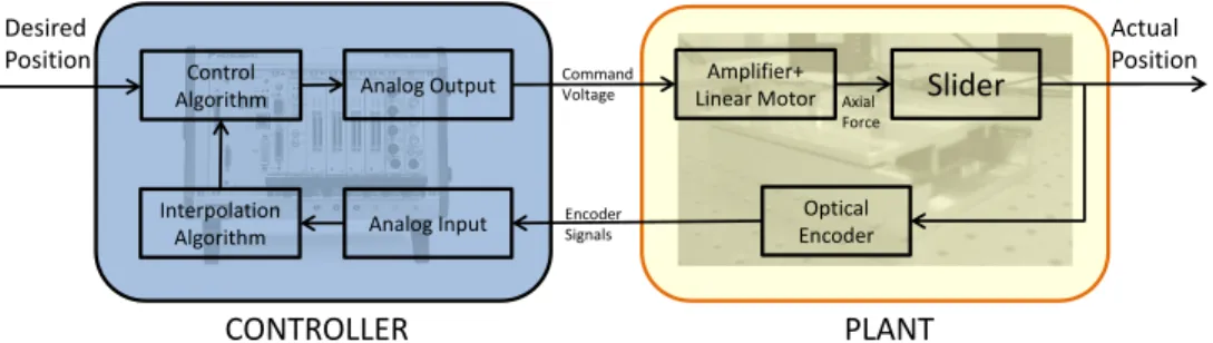
A modular single-axis stage (Figure 2.1) is composed of a stationary base and a moving slider that are connected to each other via cross-roller linear bearings. The stage is actuated by a brushless permanent magnet linear motor from Aerotech Inc. whereas the position feedback is taken from an incremental linear encoder from Heidenhain Corp. Since position is measured directly on the stage with a linear encoder, positioning becomes extremely reliable. The linear encoder has an optical scale with four micrometer in pitch leading one micrometer resolution. However for our system, the encoder resolution is increased to 25 nm using an interpolation technique. Details of interpolation procedure can be found in [8]. Travel range of the stage is 120mm and the maximum encoder traversing speed that is 500mm/s limits velocity of the system.

2.1.2

Control Setup and Testbed

In addition to the positioning system, electronic hardware and software is used for the control of the system. First a control panel should be developed to give inputs to the system and implement the developed control architecture. For this purpose, Labview software is used on a PC. The control signal is transferred to the

Amplifier+

Linear Motor Slider

Optical Encoder Desired Position Actual Position PLANT Control Algorithm Analog Input Analog Output Interpolation Algorithm CONTROLLER Command Voltage Encoder Signals Axial Force

Figure 2.2: Closed loop control setup of the single-axis system

amplifier by data acquisition system. Then, a standard current commanded six-point commutation amplifier is used for commutation of three phases of the linear motor. The position feedback is taken from the encoder by the data acquisition system. Closed loop configuration of the control setup for single-axis stage is given in Figure 2.2.

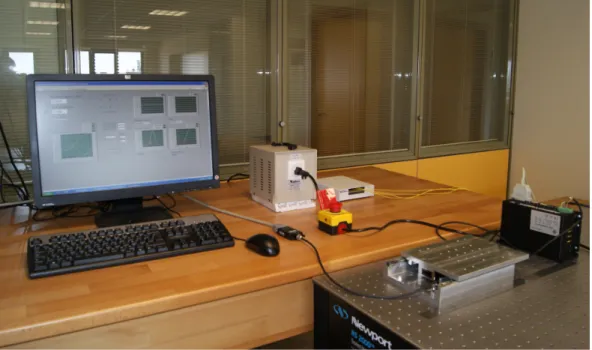
For precision positioning systems, small disturbances can deteriorate the per-formance significantly. Due to this fact, elimination of disturbances is very im-portant. One of the most important disturbance type may be the environmental vibration. In order to minimize environmental vibration, the modular stage is mounted on a vibration isolation table. Figure 2.3 shows the photograph of testbed for the single-axis slider system.

2.1.3

Multi-Axis Positioning System

In this thesis, two-axis and three-axis positioning system control is studied for multi-axis position control. The two-axis positioning system is constructed by assembling two modular single-axis stages perpendicularly as in Figure 2.4. In three-axis positioning system, a vertical axis is used in addition to two horizontal axes (Figure 2.5). In order to assemble vertical axis, an adapter is used. This adapter part is composed of an L-beam and a counterbalance system that is used for the compensation of vertical sliding mass.

Figure 2.3: Photograph of testbed for the single-axis slider system

2.2

Modeling

Mathematical model is crucial for simulation studies and theoretical analysis. In this section, mathematical model of a single-axis slider is derived. Then, the mathematical model is improved by experiments to achieve matching responses for simulations and experiments.

2.2.1

Mathematical Model of The Modular Single-Axis

Slider System

The slider system is composed of two main components as the fixed base and the sliding part. Figure 2.6 presents the sliding part of the single-axis slider system. This part is composed of aluminium top, motor track, encoder scale and one side of the bearings. The only contact mechanism in the sliding part is the linear cross-roller bearings. Moreover, the actuating force comes from motor track. These forces are shown in Figure 2.6.

Figure 2.4: Two-axis positioning system

Figure 2.6: Forces acting on the moving slider

As mentioned in the previous sections, single-axis slider system can be used in both horizontal and vertical configurations. Therefore, both configurations should be considered for the mathematical model. In Figure 2.7, forces acting on the sliding mass in the direction of movement is given for both horizontal and vertical configurations of the slider. In the free body diagram, linear bearings are modeled as part of the viscous friction component. Moreover, force ripple in the linear motor is neglected. Since use of counter balance aims to compensate weight of the sliding mass. counter balance force, fc is equal to the weight of

the sliding mass, mg. When these two forces cancel each other, horizontal and vertical free body diagrams are equivalent. Therefore, both configurations of the sliding mass can be modeled through same equations.

Idealized dynamic model of a single-axes linear stage is given in Figure 2.8 where R is linear motor resistance, L is linear motor inductance, KBEM F is back

electromotive constant, Kf orce is force constant, m is sliding mass, b is viscous

friction, e is linear motor input voltage, Kamp is amplifier gain and i is linear

motor current. In the dynamic model, ripple forces of the permanent magnet linear motor are neglected and linear bearings are modeled as viscous friction component as in free body diagram.

+" '/6/0"-/01*7"-" +" 89*0:47"+)" ;2<1/=<"-021:/97"3)"," ,," ;2<1/=<"-021:/97"3)"," '/6/0"-/01*7"-" >*2?@67"+?" 89*0:47"+)",," A/=96*034B491*"-/01*7"-1" C/02D/964B"EB2F*0" ;*0:14B"EB2F*0"

Figure 2.7: Free body diagram of the moving slider

!" #" $%&'("")" *" +" ," -.$-/01*2" 2" 3" $₄₊₅"

Figure 2.8: Dynamic model of the single-axis system

Using Newton’s law of motion, equation of motion for the sliding part can be given as

f (t) − b ˙x(t) − m¨x(t) = 0 (2.1)

Dynamic equations of the permanent magnet linear motos are found as

e(t) = Kamp(Ri(t) + L˙i(t) − KBEM F¨i(t)) (2.2)

Taking Laplace transform of (2.1), (2.2), (2.3) and arranging, plant transfer function from input voltage e to slider displacement x is found as in (2.4). Block diagram of the single-axis slider plant, P , is given in Figure2.9.

P (s) = X(s) E(s) = KampKf orce s[Lms2_{+ (Rm + bL)s + (Rb + K} BEM FKf orce)] (2.4)

Figure 2.9: Block diagram of the mathematical model

2.2.2

Model Improvement Tests

In the transfer function of the plant, viscous friction, and amplifier gain is un-known. Hence, series of experiments are conducted to obtain a numerical expres-sion for the transfer function between input voltage, e, and slider displacement, x. For this purpose, plant transfer function of single-axis slider system is approx-imated by P (s) = X(s) E(s) = GDCω2n s(s2_{+ 2ζω} ns + ωn2) e−sτ (2.5)

where GDC is DC gain, ζ is damping ratio, ωn is natural frequency, and τ is

In order to find DC gain, open loop steady state step response of the plant can be used. However, when constant step input is send to open loop plant, position response gives a ramp like output due to the free integrator in the transfer funkiction. Yet, velocity response may reach a steady state value. Since velocity is simply time derivative of displacement, the transfer function between the control input and velocity can given as in (2.6). In the equation, V (s) represent the laplace transform of velocity, ˙x(t).

Pv(s) = V (s) E(s) = GDCωn2 s2_{+ 2ζω} ns + ω2n e−sτ (2.6)

A step input with magnitude, a, is applied to the system. Laplace transform of a step input with magnitude, a, is

E(s) = a

s (2.7)

Then, the step response is found as in (2.8). Steady state value of the velocity response is derived by taking limit of the step resonse. When t → ∞, s → 0. Therefore, steady state value for velocity response, vss, becomes (2.9). Using

(2.9), the relation to calculate DC gain is obtained as (2.10)

V (s) = E(s).Pv(s) = aGDCω2n s2_(s2_{+ 2ζω} ns + ωn2) e−sτ (2.8) vss= lim s→0V (s) = lims→0 aGDCω2n s2_(s2_{+ 2ζω} ns + ωn2) e−sτ = a.GDC (2.9) GDC = vss a (2.10)

Velocity response of the plant for step input with magnitude of 0.49V is fiven in Figure 2.10. As can be observed from the figure, steady state value of velocity is about 150−155mm/s. Considering these values, DC gain is taken as 318mm.V /s. In the experiments, magnitude of the control input is critical because slider does not even move under 0.49V and velocity can not reach a steady state value before

track is finished when the control input is higher. Due to this fact, velocity response could not be provided for a longer range of motion in Figure 2.10.

0 0.25 0.5 0.75 1 1.234 0 50 100 150 200 Time [s] Velocity [mm/s]

Figure 2.10: Velocity step response

For gross estimates of ζ and ωn, velocity impulse response characteristics are

examined through series of experiments. The obtained velocity impulse response is fitted to the time solutions for the impulse response, c(t), for over-damped (ζ > 1) systems given in [9] as c(t) = ωn 2√ζ2_{− 1}e −(ζ−√ζ2_−1)ωnt − ωn 2√ζ2_{− 1}e −(ζ+√ζ2_−1)ωnt f or t ≥ 0 (2.11)

so that the system characteristics ζ and ωn are obtained as 1.1rad/s and

150rad/s. On the other hand, τ can be estimated as 0.015s by observing the closed loop step response for position loop and the controller output.

In order to compare the simulation and experimental results of the model, a PID controller is designed. Structure of the controller is

Gc(s) = Kc(1 +

1 Tis

+ Tds) (2.12)

respectively. In order to design the PID controller, Gc(s), the design objective is

chosen so that the closed loop transfer function is

Gc(s)P (s)

1 + Gc(s)P (s)

= 1 1 + sTα

(2.13)

where Tα is the desired time constant of the closed loop response. Following

the work given in [3], PID controller parameters can be chosen as

Kc = 1 GDCTdTαωn2 Ti = 2ζ ωn Td = 1 ω2 nTi (2.14) (a) (b) (c)

Figure 2.11: Step response characteristics comparison for (a) Position, (b) Posi-tion Error and (c) Controller Output

Choosing a suitable Tα, PID controller parameters are obtained using (2.14).

However, these parameters give a step response with undesirable overshoot in the simulation. Hence, by fine tuning, a new set of PID controllers are obtained so that the system shows over-damped step response characteristics both in simu-lation and experiment as shown in Figure 2.11. The system behavior with these controller parameters are similar for simulation and experiment proving that the mathematical model estimation is well enough to describe the system.

Chapter 3

Literature Survey

Recently, micro/nano-technology has been improved significantly. Micro/nano-technology related products started to be used in consumer market in addition to their applications in the science and technology world. These developments resulted in a growing interest for high precision positioning systems since precision positioning is crucial for micro/nano-technology related applications. With the rise of more complex and advanced applications requiring smaller parts and higher precision performance, demand for new control techniques that can meet these expectations is increased.

In an effort to develop a new control technique for high precision positioning systems, control of a modular positioning system is studied in this thesis. The positioning system is modular in the sense that it is constructed by the same single-axis slider to form two-axis and three-axis slider systems. Here, it is aimed to be able to control single-axis, two-axis and three-axis precision positioning sys-tems. In a single-axis precision positioning system, tracking performance is one of the most important factors. For multi-axis systems, high contouring performance is also required. Therefore, in order to achieve high precision positioning control, tracking and contouring performance should be considered. Next two sections will describe tracking control and contour control approaches used in literature.

Figure 3.1: Trajectory tracking

3.1

Tracking Control

In tracking control, the objective is moving along a desired trajectory. In Figure 3.1, an example trajectory tracking is given. In the figure, the left plot shows a better tracking response compared to the one at the right since most of the actual movement is along the desired trajectory. Most commonly used tracking control method is feedback control with PID [10, 5, 11, 12, 13]. Sliding mode controller is also used as a feedback tracking control in [14, 15]. Almost all systems employ feedback as a part of tracking control however substantial improvement of tracking accuracy is achieved by addition of forward control. Several feed-forward control schemes developed to improve tracking accuracy in literature such as zero phase error tracking control (ZPETC) [16, 17, 18], feed-forward friction compensation [19, 14, 20] and iterative learning control (ILC) [3, 21].

Tracking performance of a ZPETC system is sensitive to variations in plant parameters and modeling errors since ZPETC design is based on pole/zero can-cellation and phase cancan-cellation [16]. Friction compensation techniques generally incorporate a system identification process that should be repeated if system pa-rameters change. Tan et al. [3] claims that specifying a plant model for ILC via zero phase filtering is not necessary due to the principle of self-support that is argued in [22]. Since the stored control signals reflect the plant characteristics, ILC can improve tracking performance of a system even the plant structure and

nonlinearities are unknown [23]. However, the system should execute the same task repetitively to be able to implement an ILC scheme.

Iterative learning control can be applied to the systems that repeatedly ex-ecute the same operation. By applying it, experience gained from the repeated execution is used to improve the performance of the system. Considering this fact, iterative learning control schemes are suitable to be used in high precision con-trol of linear motors. In the literature, there are a several cases in which various iterative learning control schemes are applied in combination with some other control techniques for linear motor control purposes. In [24], frequency based ILC, H∞ based ILC and second order ILC approaches are considered for linear

motor motion system. Scholten simulated these three alternatives and compared their performance. As a result Scholten concluded that the best performance is achieved by second order ILC although all of the ILC types improved the per-formance of the system with conventional control schemes. In all cases, Scholten claims that the tracking error is decreased compared to the ones with the conven-tional controllers. In [25], internal model based iterative learning control for linear motor motion systems are considered. According to Fan et al., the main reason for linear motor not to reach high tracking accuracy is nonlinear disturbances. In order to achieve high tracking accuracy by rejecting the nonlinear disturbances, they combine the iterative learning control with internal model control. Hence, they claim that ILC based on internal model control can guarantee the robust performance and high tracking accuracy with the experience obtained from early stages of learning.

Linear parameter varying iterative learning control for linear motor systems is explained in [26]. In this paper, the basic assumption is that the dynamics of the system change between iterations. According to Butcher et al., permanent mag-net linear motors are affected by periodic, position dependent force disturbance. Although these periodic disturbances can be eliminated by using ILC, if the initial position of the system changes, the disturbance changes so that learned input will not lead to the optimal tracking. For this reason, they proposed linear parameter varying ILC for linear motor control purposes. As a result of their work, it is claimed that better results are obtained using the proposed method compared to

the one using linear time invariant ILC. Another research on iterative learning based control of linear motor is given in [3]. They combined relay tuning and ILC based on zero-phase filtering to control high precision linear motor in their work. Tan et al. improves the tracking performance of the linear motor by applying ILC based zero-phase filtering as feedforward controller to the relay tuned PID feedback controller. As a result of experiments, the proposed method in their work has higher effectiveness to be used in linear motor control purposes.

3.2

Contouring Control

!"

!"

!"

!

)

!

W)

K)

Figure 3.2: Tracking and contour error

In literature and commercial products, contouring control is achieved by im-proving tracking of the systems. Generally, imim-proving tracking accuracy of an individual axis also increases contouring accuracy of the multi-axis system. How-ever, reducing tracking error does not necessarily result in a reduction in contour error in nonlinear cuts [27]. In some cases, decreasing the tracking error may not decrease the contour error; it may even deteriorate the contouring performance. This can be observed in Figure 3.2. The axial errors are defined as the distance between the desired position, R and the actual position, Pa. Contour error, ε,

desired contour as shown in Figure 3.2. When the actual position is moved to P_a0 from Pa decreasing the axial tracking errors from ex and ey to e0x and e

0

y, contour

error, ε increases and becomes ε0. Therefore, special control approaches should be employed for contour control since in contouring applications contour tracking is more important then trajectory tracking.

For contouring control, first the system should have a good tracking control in each single-axis. Then, contour control can be accomplished through different MIMO control schemes. Koren [28] proposed the cross-coupled control (CCC) structure that focuses on eliminating the error in contouring rather than tracking in individual axes, This method is proven to reduce contour error significantly. Since the introduction of CCC, many controllers based on CCC has been de-veloped. Other than CCC and its modified versions, model predictive contour control for biaxial feed drive systems is presented in [2]. Next subsections de-scribe model predictive contouring control and CCC and CCC based contouring controls. Then, contour error models are discussed.

3.2.1

Cross-coupled Control

For contour control, Koren proposed cross-coupled control (CCC), which is the first control scheme to consider mutual dynamic effect among all axes, in [9]. Cross-coupled control scheme introduced the notion of finding the contour error from multiple error signals, applying some form of control to the combined signal, and feeding the new signal back into the respective systems. This concept is a special type of multi input multi output (MIMO) control which aims to decrease the contour error. Block diagram of this control scheme is given in Figure3.3. In the block diagram, Cx and Cy are coupling gains whereas ε, ex, ey are the

contour error, x-axis tracking error and y-axis tracking error respectively. As can be observed form Figure3.3, contour error is obtained through (3.1)

)P4)2<" 5B496" (**F341U"A/960/BB*0" /-")P4)2<" A0/<<PA/=5B*F" A/960/BB*0" A_)" A)" A_N" A_N" )F" *)" *_N" T" K"P" K" P" K" P" P" K" K"K" NF" (**F341U"A/960/BB*0" /-"NP4)2<" NP4)2<" 5B496" )_" N_"

Figure 3.3: Block Diagram of CCC

Although CCC is first introduced with constant gains in [28], the term CCC is generally used for CCC with variable coupling gains as proposed in [27]. The next section describes the proposed modifications and combnations of CCC.

3.2.2

Variations and Combinations of CCC

Since the introduction of CCC, it has been modified and combined with different control techniques. In this section development of CCC to its form that is used today will be outlined. Then, other control designs integrating another control schemes to CCC are examined.

First, Koren introduced CCC around 1980s [28]. This method was the first approach to use a specific controller for contour control instead of improving tracking accuracy only. In this approach, contour error is acquired by combining axial error signals and feeding the new signal back into the respective systems after applying some control. Then, this work was followed by several papers from Kulkarni and Srinivasan [29, 30, 31, 32]. Srinivasan and Kulkarni came out with a new CCC design which separated the contour error into two different signals for the x and y axis respectively in 1990 [33]. After this design, Koren introduced the variable-gain cross-coupling controller which is currently the most widely used design in industry [27]. Recently, widely used CCC method is also adapted as in

)P4)2<"LB496" A0/<<PA/=5B*F" A/960/BB*0" A)" A)" A_N" A_N" )F" *_)" *N" T" K" K" K" P" P" K" P" K" NF" NP4)2<"LB496" )" N_" K" K"

Figure 3.4: Block Diagram of Position Based CCC

Figure 3.4. This position based configuration of CCC is proposed in [34].

Tracking control and contour control are two essential parts of contouring. In the literature, control schemes for tracking and contour control are combined in various ways to improve contouring. Some examples can be given as observer-based CCC [35], cross-coupled model reference adaptive control[36], cross-coupled iterative learning control (CCILC) [21], CCC with disturbance observer and ZPETC [18], CCC with friction compensation [14] and CCC with ILC [21, 37, 38].

3.2.3

Contour Error Estimation Models

Since CCC based control schemes require contour error as the control parameter, there is a need for a contour error model in real time. Contour error is defined as the distance between actual position and nearest position on the contour [1]. Contour error can be calculated easily for linear contours. However, this calcula-tion is very complicated for nonlinear contours, especially during the operacalcula-tion. Hence, some approximations have been used to calculate a nonlinear contour er-ror. The most common one is using the circular contour assumption suggested by Koren et al. [27]. Yeh and Hsu [1] proposed another method that approximates contour error as the vector from the actual position to the nearest point on the line that passes through the reference position tangentially. The latter approach

has several advantages over the former as computational efficiency, suitability for arbitrary contours and convenience for multi-axis implementation [1]. Recently, an iterative approach is develop to improve estimated contour error in [39]. For the estimation of contour error, there are two basic models circular contour ap-proach and tangential contour error approximation. Next two parts will briefly present these approximations.

3.2.3.1 Circular Contour Assumption

In this approach any arbitrary contour is separated into parts with radius of curvature ρ and these parts are approximated by circles. Since contour error for a circular contour is the difference between the distance from the actual position to the center of the circle and radius of the circle, contour error for an arbitrary contour can be written as (3.2)

ε =

q

(x − x0)2+ (y − y0)2− ρ (3.2)

where (x0, y0) and (x, y) denote center of the curvature and actual position,

respectively. Expressing the actual position with respect to reference position and axial tracking errors, ex, ey and using Taylor expansion, approximated contour

error becomes (3.3)

ε = (cos θ + ey

2ρ)ey − (sin θ − ex

2ρ)ex (3.3)

where θ is traversal angle of motion and ρ is the radius of curvature at the point. In (3.3), ρ is infinity for linear contours. Moreover, ρ becomes the constant radius of circle for circular contours.

Figure 3.5: Geometrical Relations of Contour Error (adopted from[1])

3.2.3.2 Contouring Error Vector Approach

Contour error vector approach can be explained through the geometrical relations in the multi-axis motion control system given in Figure3.5. In the figure, −→e is tracking error vector, −→ε is estimated contour error vector, −b

→_{ε is contour error} vector, −→t is normalized tangential vector, −→n is normalized normal vector, P is actual position and R is reference position. In this approach, contouring error −→ε is defined as the vector from the actual position to the nearest point on the line that passes through the reference position tangentially with direction−→t [1]. This approach estimates contour error vector very closely when tracking error is small enough. Looking at Figure3.5,−→ε is equal to h−b

→_{e , −}→_{n i where h., .i is inner product} operator. Hence, relation between−→ε and −b

→_{e can be obtained using inner product.} Furthermore, the contour error is calculated as |−→ε | =b

P

i

Ciei(i = x, y, z) where

Ci is coupling gain and ei is the corresponding axial tracking error. Considering

these two representations of estimated contour error vector, cross coupling gains (Cx, Cy, Cz) in terms of normalized normal vector (−→n = [nx ny nz]T) are found

as Ci = ni(i = x, y, z, ). In other words, cross coupling gains at a point are the

3.2.4

Model Predictive Contouring Control

This control method uses model predictive control strategy that utilizes an ex-plicit process model and tracking error dynamics to predict the future behavior of a plant. Model predictive contouring control delivers a novel approach towards improving contour accuracy. As mentioned in previous section, contour error can be estimated as the vector from the actual position to the nearest point on the line that passes through the reference position tangentially. Considering this the error components orthogonal to the desired contour curves are more important than tracking errors, and hence, control inputs are found from the normal and tangential components of the axial errors.

Figure 3.6: Model Predictive Contouring Control Diagram [2]

Block diagram of the proposed contouring control system is as in Figure 3.6. In the MPCC box, a minimization problem given in (3.4) is solved. ρcn and

ρct are weighting factors to adjust the importance of the error component in

the orthogonal and tangential directions, respectively, ρn and ρt are weighting

factors used to adjust the control inputs in the normal and tangential directions, respectively, and uxj ; uyj ; unj and utj are the jth control inputs in the x, y, n

J = ρcn Hp X j=HM enj2+ ρct Hp X j=HM etj2 + ρn Hp X j=HM unj2+ ρcn Hp X j=HM utj2 (3.4)

3.3

Conclusion

To sum up, tracking control and contour control are two essential parts of con-touring. In the literature, control schemes for tracking and contour control are combined in various ways to improve contouring. Model predictive contouring control method provides an efficient contour control. However, cross-coupled control has been used for this purpose for a longer time and effectiveness of this method is proven by many researchers. Moreover, model predictive contouring control is only used for biaxial systems although it is claimed that the controller can be extend to multi-axis systems. In this thesis, developed controller should work on multi-axis systems that can be have more than two axes. Moreover, using ILC is beneficial for our system since it is modular. The slider system can be used for many positions, being able to improve its tracking is an advantage of ILC when position of the modular slider is changed. This way, system can show good performance even its position is changed or any other slider is assembled on it.

For contour error estimation models, although two described approaches give similar results in terms of contouring accuracy, contour error vector method has several advantages over the circular contour assumption. Firstly, it is computa-tionally more efficient. An extensive study on the computational efficiency of the contour error vector approach over the circular contour approach is given in [1]. Moreover, with contour error approach, coupling gains can be computed easier for an arbitrary contour. Also, implementation of contour error vector approach to multi-axis systems is accomplished by the same procedure used for two-axis systems and this procedure is well established. Therefore, contour error vector approach is more suitable for multi-axis systems.

Chapter 4

Development of The Control

Algorithm

The multi-axis precision positioning system is constructed by assembling modular single-axis stages. The single-axis stage is modular in the sense that couple of them can be assembled together to form two or three-axis positioning systems. Therefore, a single-axis stage can be used as x-axis, y-axis or z-axis. Model parameters of a single-axis stage change depending on which axis it is used for. For this reason, an iterative learning controller is designed to improve tracking performance of a modular single-axis stage after a feedback controller is found as explained in Chapter 2. Use of iterative learning control also helps modular sliders adapting to repeated disturbances and nonlinearities of the axis they are used for.

In this chapter, an new method based on CCC and ILC which benefits from the contouring error vector approach is presented. A preliminary study for using CCC and ILC together is given in [38]. Also, Barton et al. worked on controllers incorporating CCC and ILC for contours combining lines and circles on a two-axis system in [21, 37]. As one of the main contributions, proposed method also benefits from the contouring error estimation vector approach. The method presented here is computationally more efficient, more suitable for coupling gain

calculations of arbitrary nonlinear contours and easier to implement on multi-axis systems than traditional approaches. Moreover, our method utilizes ILC via zero-phase filtering so that the design process for ILC is practical and suitable for modular systems. Other important contribution of the method is that this is the first time CCC and ILC is used together to achieve nanometer level precision. Moreover, the controller is not only designed for two-axis systems but also multi-axis systems (two or more).

Here, an extended study on our work presented in [40] is given. Next section describes zero filtering based ILC. Cross-coupled control implementation is dis-cussed in the second section. Then, the proposed learning based cross-coupled controller is explained. Stability and convergence of the controller is examined in the last section. Effectiveness of the control design is verified with simulations and experiments on two-axis and three-axis positioning systems using nonlinear contours. Simulation and experiment results are provided in Chapter 5.

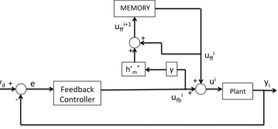
Figure 4.1: Block Diagram of ILC via Zero-Phase Filtering with Feedback Con-troller [3]

4.1

Iterative

Learning

Controller

via

Zero-phase Filtering

ILC is a technique for improving the transient response of a system that operates repetitively. ILC can often be used to achieve perfect tracking, even when the model is uncertain or unknown and there is no information about the system structure and nonlinearity [23]. ILC based on zero phase filtering is a practical and efficient implementation of ILC [3].

(**F341U" A/960/BB*0" LB496" '&'`!Q" K @b+c" K K" P" N_F" _*" =_S2_" =_R2_" K" K" =_R2K\_" N₂" =2_" a"

Figure 4.2: Reorganized Block Diagram of ILC via Zero-Phase Filtering with Feedback Controller

Block diagram of zero-phase filter based iterative learning controller is given as Figure 4.1 in [3]. In Figure 4.2, a reorganized version of this control scheme is provided to see it in a traditional block diagram form. In both diagrams, superscript i is iteration number whereas ui

f f, uif b and yi are feed forward control

signal, feedback control signal and system output at ith _{iteration. Moreover, y} d

is the desired system output which does not change between iterations. h0_m∗ is algebraic averager and γ is learning gain. The feed forward control signal for ith iteration is calculated using the feed forward and feedback control signals of the previous iteration that are shown as ui−1_{f f} and ui−1_{f b} respectively. The learning update law can be given as in (4.1)[3].

ui_{f f}(k) = ui−1_{f f} (k) + γ 2M + 1 M X j=−M ui−1_{f b} (k + j) (4.1)

where k is the time index, γ is the learning gain and M is the length index of zero phase filter. Detailed guidelines for the design of parameters γ and M can be found in [3]. For our system, M is used as 11 and γ is taken as 0.2. Although choosing suitable M and γ values is crucial for convergence, a suitable set of M and γ values can be used for many processes. For example, the same M and γ values are used in all our single-axis, two-axis, three-axis simulations and experiments. In the Simulink implementation, first the block diagram is executed, then a learning m.file is executed for each iteration. The learning m.file is the implementation of (4.1). Simulink block diagrams and real-time Labview VI’s and front panels of single-axis ILC implementation are given in Appendix A and B, respectively.

4.2

Cross-coupled Control with Contouring

Er-ror Vector Approach

)P4)2<" 5B496" (**F341U"A/960/BB*0" /-")P4)2<" A0/<<PA/=5B*F" A/960/BB*0" A_)" A_)" A_N" A_N" )_F" *_)" *N" T" K"P" K" P" K" K" K" K"K" N_F" (**F341U"A/960/BB*0" /-"NP4)2<" NP4)2<" 5B496" )" N" K"

Figure 4.3: Block Diagram of Cross-coupled Control with Contouring Error Vec-tor Approach

Cross-coupled controller is designed in order to consider the effects between axes. Contouring error vector approach is used to calculate the coupling gains

of the cross-coupled controller. Block diagram of the cross-coupled controller is given in Figure 4.3.In the block diagram, Cx and Cy are coupling gains whereas

ε, ex, ey are the contour error, x-axis tracking error and y-axis tracking error

respectively. −10 −5 0 5 10 15 20 −5 0 5 10 x−axis y−axis Contour Normal Lines Tangent Lines

Figure 4.4: 2D contour with its tangents and normals

In contouring error vector approach, contouring error −→ε is defined as the vector from the actual position to the nearest point on the line that passes through the reference position tangentially with direction−→t [1]. Cross coupling gains at a point are calculated as the elements of unit normal vector of the contour at that point. Therefore, cross-coupling gains are

Ci = ni (i = x, y, z, ) (4.2)

where (Cx, Cy, Cz) are coupling gains and (−→n = [nx ny nz] T

) is the unit normal vector. For the control implementation, coupling gains are found through the developed coupling gain m.file. To find the coupling gains, normals of the contour at each reference point is found. In Figure 4.4, a two dimensional contour is shown with its tangents and normals at some reference points. Components of the unit normal vector at a reference point gives the coupling gains.

A)" A)" AN" AN" )_F" *_)" *N" T" K"P" K" P" K" K" K" K" K"K" N_{F" (**F341U"A/960/BB*0"} /-"NP4)2<" NP4)2<"5B496" )_" N" (**F341U"A/960/BB*0" /-")P4)2<" A0/<<PA/=5B*F" A/960/BB*0" )P4)2<" 5B496" '*+/0N" 8#A" =_R)2P\" =_S)2P\" =_S)2" =R) 2" K" K" =_S)2" '*+/0N" 8#A" =_RN2P\" =_SN2P\" =_SN2" =RN2" K" =_SN2" K" K" =_RN2" =_R)2"

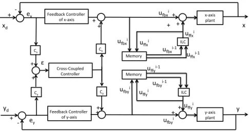
Figure 4.5: Learning Based Cross-coupled Controller for Two-axis Systems

4.3

Learning Based Cross-coupled Controller

The control system is intended to be modular considering being able to inter-change the stages without changing the control system. For modularity concerns, ILC is chosen for improving tracking performance since controller structure does not change with changes in plant model structure and parameters. Moreover, use of ILC is beneficial for modular systems to compensate for changes after the assembly. For example, when a modular stage is assembled on top of another, weight of the sliding mass changes. Since there are only two design parameters in single-axis control scheme of ILC via zero-phase filtering, the implementation is practical. Moreover, contouring error vector method is chosen to use with CCC since it is computationally more efficient. As mentioned before, encoders of the positioning system have been interpolated to achieve nanometer resolution. This procedure is accomplished without any extra hardware. Due to this fact, there is a trade of between resolution of the encoders and the computational effort in the control loop. Therefore, it is aimed to minimize computational effort in the con-trol loop to maximize encoder resolution. Using contouring error vector technique also makes the control method more suitable to implement on multi-axis systems and to operate with arbitrary nonlinear contours. To sum up, a control method featuring CCC and ILC via zero phase filtering has been developed incorporating the contouring error vector estimation technique (Figure 4.5).

AM" AZ_{" A"} A11" C" B" B" N" '&'\!J" B ^_+`" B B" I" 0;" *" >M2" >L2" B" B" >L2BW" 0" >2_" ]"

Figure 4.6: Learning Based Cross-coupled Controller for Multi-axis Systems

4.4

Stability and Convergence

Analizing the stability of a control design is important to ensure that the con-troller can stabilize (or won’t destabilize) a given system. Design of the proposed control system can be considered through three steps which are designing feed-back controllers for each axis, a cross-coupled controller and iterative learning controllers for each axis while considering the cross-coupled control signals. A generalized block diagram of the presented control for multi-axis systems is given in Figure 4.6. Symbols and their explanations are given in TABLE 4.1

!"# !$_# %# &'# (# )# *+# ,'# *#

Figure 4.7: Block Diagram of Uncoupled System

Firstly, a stabilizing controller can be designed for each single-axis slider. Then, the designed cross-coupled controller should be stable. For cross-coupled systems, stability can be analyzed through a term called contour error transfer function (CETF). Concept of CETF is introduced by Yeh and Hsu in [41] as

Table 4.1: Parameters

Symbol Description

rd = [rdx, rdy, rdz, ...]T desired input trajectory

r = [rx, ry, rz, ...]T output trajectory

e = [ex, ey, ez, ...]T axial tracking error

e = [eux, euy, euz, ...]T uncoupled axial tracking error

ui _{= [u}i

x, uiy, uix, ...]T axial driving signal at ith iteration

ui_{f b} = [ui_{f bx}, ui_{f by}, ui_{f bz}, ...]T combined control signal

ui_{f f} = [ui_{f f x}, u_{f f y}i , ui_{f f z}, ...]T feedforward control signal at ith iteration

C = [Cx, Cy, Cz, ...]T coupling gains

Cf b = diag{Cf bx, Cf by, Cf bz, ...} feedback controller

P = diag{Px, Py, Pz, ...} axial controlled plant

Ccc cross-coupled controller

γ learning gain

h0_m∗ algebraic averager for ILC

ε contour error

εu uncoupled contour error

the relationship between a coupled (Figure 4.8) and uncoupled (Figure 4.7) sys-tem. Coupled system refers to a system controlled by cross-coupled controller and uncoupled system refers to the same system only without the cross-coupled controller. To derive the CETF, contour error should be derived for systems without and with CCC as εu and ε, respectively. Contour error for uncoupled

system can be derived as follows

eu= rd− r = rd− P .Cf b.eu = (I + P .Cf b) −1 .rd (4.3) εu = CT.eu = CT.(I + P .Cf b) −1 .rd (4.4)

!"# !$_{# !#} !_%%# &# '# '# (# '# )# *+# ,# *#

Figure 4.8: Block Diagram of Coupled System

For the coupled system, contour error is calculated as follows:

e = rd− r = rd− P .(Cf b.e + C.Ccc.CT.e) = (I + P .Cf b+ C.Ccc.CT)−1.rd (4.5) ε = CT.e = CT.(I + P .Cf b+ C.Ccc.CT)−1.rd (4.6)

CETF, the relation between uncoupled and coupled system is as given below as H

ε = H.εu (4.7)

Combining (4.4), (4.6) and (4.7), then using matrix inversion lemma, CETF is found as H = 1−CT.(I + P .Cf b) −1 .[P−1+ C.Ccc.CT(I + P .Cf b) −1 ]−1 (4.8)

After some simplifications, CETF becomes

H = 1 1 + CT.(I + P .Cf b) −1 .P .Ccc.C = 1 1 + PeCcc (4.9) where Pe = CT(I + P .Cf b) −1

.P .C and can be considered as an equivalent controlled plant. In Pe, C is the cross coupling gains vector and the gain values

are changing between -1 and 1 throughout the motion. Therefore, the equivalent controlled plant has varying parameters. Although these gains vary during the motion, they are not iteration varying because they are related to the reference contour. Considering CETF, H, as the sensitivity function, the cross-coupled controller can be designed using conventional single-input-single-output control methods. Therefore, a stabilizing controller Ccc can be designed for this system

using traditional feedback stability and robustness techniques after each single-axis loop is designed to be stable. Moreover, according to the theorem given in [41], cross-coupled system is internally stable if single-axis feedback controllers achieve internal stability for each axis and the cross-coupled controller keeps the equivalent control system(Ccc, Pe) internally stable while the coupling gains vary.

Block diagram of the equivalent control system is given in Figure 4.9

!

#

&_'#(# )#

&#

Figure 4.9: Block Diagram of Equivalent Control System

Convergence of the ILC via zero phase filtering on a cross-coupled system can be shown extending the convergence analysis for the single-axis system given in [3]. For the convergence of analysis, some assumptions should be made. Firstly, single-axis plants should be stabilizible and internally stable as well as the cross-coupled control system itself. Furthermore, the number of inputs should be equal to the number outputs in the system. There should be unique desired input ud

for a desired trajectory rd. Considering control signals as an indication of plant

dynamics, system dynamics, ui_{can be separated into its repeated and unrepeated}

components as ud

R and uiN R, respectively where the unrepeated part is bounded

by h0_m∗ ui

N R ≤ ε∗ for ∀i.

According to the theorem given in[3], ui

f f approaches udR as i increases when

ε∗ → 0 if the assumptions are satisfied and a task is performed repeatedly. In real aplications, ε∗ is very small and can be assumed as ε∗ ≈ 0. Therefore, while ε∗ tends to zero lim i→∞u i f f = u d R (4.11)

For the proposed control system, ILC via zero phase filtering is applied to the all single-axis loops. Since all axis trackings are convergent, the contour error is also convergent. Convergence of the RMS (root mean square) contour error is shown in Figure 4.10 for both simulation and experiment. Convergence analysis for simulations and experiments are performed for the trajectories given simulation and experiments chapter. As can be observed from (a) of Figure 4.10, RMS contour error for simulations converges to a value which is very close to zero. For the experiments, convergence is not as smooth as the simulations due to unrepeated disturbances and nonlinearities that are not modeled. RMS contour error converges to a value around 30nm. Convergence to 30nm RMS contour error value can be considered as a good result since encoder resolution used for the experiments is 25nm.

0 5 10 15 20 25 30 35 40 0 5 10 15 Iteration Number RMS Contour Error [nm] (a) 0 5 10 15 20 25 30 35 40 20 30 40 50 60 70 80 Iteration Number RMS Contour Error [nm] (b)

Chapter 5

Simulation and Experiment

In order to verify the performance of the positioning system, simulation analysis and experiments are conducted for single-axis, two-axis and three-axis positioning systems. For both simulations and experiments, velocity profiling has been used to generate individual-axis reference trajectories. Generic s-curve method is em-ployed for this purpose. In this chapter, trajectory planning used for this thesis is explained. Then, simulation and experimental results of single-axis, two-axis and three-axis system are given respectively.

5.1

Trajectory Planning

With the increased demand from the industry, positioning systems are required to have both high precision and high speed operation capabilities in recent years. However, uncontrolled accelerating or decelerating motion causes residual vibra-tions during high-speed operation. Hence, the accuracy of the system decreases whereas the settling time increases. However, residual vibrations can be prevented by planning the reference trajectory of the system in a way that acceleration and deceleration phases are smoothed out [42, 43, 44]. This kind of trajectory plan-ning is mostly done by various optimization methods based on the time derivative of the acceleration (i.e., jerk).

Figure 5.1: A Pulse Shaped Jerk Profile and Its First, Second and Third Integrals as Acceleration, Velocity and Position Profiles

In this section, motion of the stage is planned so that the stage moves smoothly, increasing the accuracy and speed of the motion. Figure 5.1 shows jerk, acceleration, velocity, and position profiles of a typical point to point tra-jectory, called as s-curve profile. The motion is composed of three regions. These are acceleration region (I to III), constant velocity region (IV), and decelerating region (V to VII). At region II, the maximum acceleration and at region VI, the minimum acceleration is reached and the acceleration is kept constant at these phases of the motion. However, for our system, since the track of the motion is limited by 120mm, it is impossible for the slider to reach the maximum possi-ble acceleration and velocity during its motion between any two points. Hence, regions II, IV, and VI in Figure 5.1 are not present so that the motion is ac-complished in maximum and minimum jerk regions only. In the single-axis slider system, magnitudes of maximum and minimum jerk are the same and they can be chosen between 0 to 5000mm/s3_{. Moreover, durations for maximum and}

min-imum jerk regions (I, III, V, and VII) are calculated automatically depending on the specified jerk magnitude and the desired position value.