Application of the Kramers
–Kronig Relations to Multi-Sine
Electrochemical Impedance Measurements
Chen You,
1,=,*
Mohammed Ahmed Zabara,
2,=Mark E. Orazem,
1,**
and Burak Ulgut
2,***
,z1
Department of Chemical Engineering, University of Florida, Gainesville, Florida 32611-6005, United States of America
2Department of Chemistry, Bilkent University, 06800 Ankara, Turkey
Impedance spectra obtained by fast Fourier transformation of the response to a multi-sine potential perturbation are shown to be consistent with the Kramers–Kronig relations, even for systems that are nonlinear and nonstationary. These results, observed for measurements on a Li/SOCl2battery, were confirmed by numerical simulations. Consistency with the Kramers–Kronig relations
was confirmed by use of the measurement model developed by Agrawal et al. and by a linear measurement model approach developed by Boukamp and implemented by Gamry. The present work demonstrates that application of the Kramers–Kronig relations to the results of multi-sine measurements cannot be used to determine whether the experimental system satisfies the conditions of linearity, causality and stability.
© 2020 The Author(s). Published on behalf of The Electrochemical Society by IOP Publishing Limited. This is an open access article distributed under the terms of the Creative Commons Attribution 4.0 License (CC BY,http://creativecommons.org/licenses/ by/4.0/), which permits unrestricted reuse of the work in any medium, provided the original work is properly cited. [DOI:10.1149/ 1945-7111/ab6824]
Manuscript submitted November 8, 2019; revised manuscript received December 12, 2019. Published January 20, 2020.
Electrochemical Impedance Spectroscopy (EIS), namely mea-suring the frequency-dependent complex impedance as a function of frequency, has become a fundamental technique for analyzing electrochemical systems. The information-rich response of EIS enables the determination of properties for various electrochemical phenomena in broadly varying systems.
The power of EIS relies on the ability to study the electro-chemical phenomena on a wide timescale. It is utilized very heavily in all areas of electrochemistry, from energy storage and conversion1–5 to coatings,6,7 from physical electrochemistry8–10 to corrosion .11,12In all cases, EIS data allow decoupling phenomena occurring at different timescales in the system. As examples, for batteries and fuel cells, the area difference of the electrodes allow separation of the behavior of two electrodes,13,14 for corrosion studies, the polarization resistance of the metal can be obtained without any contribution from the solution resistance15and, in cases where the metal is coated, the coating properties can be isolated.12,16 These separations are only possible because characteristic timescales (typically RC time constants) for these phenomena are clearly separated.
Since the resolving power of the technique comes from the ability to interrogate events occurring at different timescales, the accessible range of frequencies is an important parameter to discuss. The range of frequencies is rarely limited by instrumentation. On the high-frequency side, manufacturers of electrochemical impedance spec-troscopy equipment specify instruments to have a maximum frequency as high as 8 MHz with a potentiostat17 and 32 MHz17 without. While it is true that, with the correct resistor connected across the instrument cables and correct geometry, there may be an accurate measurement at such high frequencies, measurements with practical systems including cable limitations are typically only useful up to 50 kHz or less. The low-frequency side is more interesting. Instrumentally, there is no limitation on how slow a measurement can be made. Manufacturers’ limits on the low side, when they exist, are bound by factors such as time between data points, USB sleep times, etc, which can be modified easily if/when necessary. However, most of the time, the principal limitation is sample stability and, more often, stationarity. Instrument software typically allow for frequencies as low as 10μHz, which corresponds to 105s per period, roughly 27.8 h. Given the need for measurement
of multiple cycles, at least 56 h are necessary for a measurement at a frequency of 10 μHz. Most electrochemical system are not sta-tionary over a period of days to weeks.
In an effort to decrease the measurement time, multi-sine, or more generally, Fourier Transform techniques have emerged as an alter-native. Multi-Sine Electrochemical Impedance Spectroscopy (MS-EIS) was introduced in the late 1970s18,19 as a technique that can improve data acquisition and can shorten the experiment duration. It has been implemented by instrument manufacturers20,21and used by several research groups to obtain impedance results of various electrochemical systems.22–26
Unlike the conventional step-sine EIS in which excitation signals are applied at each frequency separately, MS-EIS excites the sample by one composite signal containing numerous frequencies intended for investigation. Application of the Fast Fourier Transform (FFT) on the full signal yields a frequency response from the multi-sine signal. The impedance is calculated from ratio of the voltage to the current at each frequency. Fourier Transform techniques are routinely used in analytical chemistry, especially in techniques where a large number of averages are necessary. Instruments that perform FTIR27 and FTNMR28 are commonplace in chemistry laboratories.
Thefirst application of MS-EIS in the literature was reported by Smith et al., who applied pseudorandom white noise excitation signals to measure the self-exchange rate constants for Cr(CN)6
4−/Cr(CN) 6
3−system.18
The technique was named Fourier Transform Admittance due to the reliance on FFT to obtain the admittance values. They also described the data processing involved for FFT impedance and highlighted the advantages of using the technique.19
Later several studies utilized the technique to obtain the electro-chemical impedance of various systems. Smyrl29 and Smyrl and Stephenson30 describe “digital impedance for faradaic analysis” (DIFA), an input spectrum consisting of superimposed sinusoids such that the higher frequency members are harmonics of the lowest frequency, and applied the technique to study corrosion of copper in HCl. Later Wiese et al.31described the working principles of Fourier Transform Impedance spectrometer in the frequency range from 1 Hz to 105Hz. They report that impedance spectra were obtained within few seconds. Few years later, Schindler et al. developed phase-optimization for the excitation signal to optimize the response. The perturbation signal used was a superposition of sine waves with properly chosen frequencies.32,33 Gabrielli et al. did a comparison study for the impedance results of single sine wave and white noise excitation.34They stated that the both techniques allow for accurate impedance measurements and that the white noise yields shorter
zE-mail:[email protected]
=These authors contributed equally to this work. *Electrochemical Society Student Member. **Electrochemical Society Fellow. ***Electrochemical Society Member.
measurement time only if linear spaced frequencies are tolerable in the lowest decade.
Another approach was taken by Gheem et al. in which a broadband periodic excitation signal, called odd random phase multi-sine, was introduced as a technique to characterize non-linear and non-stationary systems.35,36 As stated by the authors, the technique allows for differentiation between non-stationarity and non-linearity in the system and has been applied to coatings and corrosion systems.37,38
In addition to the MS-EIS techniques, there have been numerous studies involving signals that are not generated by adding sine waves. Relaxation Voltammetry39 is one of the early examples where a simple open circuit voltage decay measurement has been employed as the signal used in order to calculate the impedance at low frequencies. The voltage measured can be Fourier transformed into the frequency domain in order to obtain the spectrum. Though this measurement is simple, the frequency domain signal is very broad and continuous, decreasing the signal power at any given frequency, and thus creating issues with signal-to-noise. The extreme case for signal-to-noise issues come in cases where the signal is simply a potential step function.23Once the derivative of the step is taken, the result is a Dirac function, which is effectively white in the frequency domain. Though this is shown to work in very-low-impedance systems where there is plenty of current signal, it is also shown to have problems.40
There are several commercial implementations of MS-EIS. In all implementations, the goal has been to decrease the time requirement of the measurement.20,21,41 In the low-frequency region, properly designed signals have been shown to decrease the time requirement of the measurement by up to factors of 4.
The fundamental assumptions behind any EIS measurement are that the measurements are linear, stable, and causal.42The causality and the stationarity conditions can be checked through compatibility with the Kramers–Kronig relations. The Kramers–Kronig relations relate the real and the imaginary component of the obtained impedance values, e.g.,
( )w
ò
( ) ( ) [ ] p w w = - -¥ ¥ Z Z xZ x Z x dx 2 1 r r j j , 0 2 2Equation 1 shows that real component of impedance Zr can be predicted from an analytical function of the imaginary component if the conditions of linearity, stability and causality are not violated. Any deviation from the Kramers–Kronig transform can be attributed to the presence of nonlinearity or non-stationarity in the measurement.
As can be seen from Eq. 1, direct application of the Kramers–Kronig relations requires integration over frequency ran-ging from zero to infinity. Due to the finite frequency range accessible in practical EIS measurements, various approximations are employed in order to check compatibility with Kramers–Kronig relations. The implementations either rely on fitting the data to generic Kramers–Kronig-compatible circuit elements, or extrapola-tions of the data to the rest of the frequency domain.
Two implementations that rely onfitting generic Kramers–Kronig-compatible models to the data are the measurement model method43,44 and the Boukamp method.45 The measurement model is based on fitting electrical circuits corresponding to the Voigt model, which is consistent with the Kramers–Kronig relations. The Boukamp method is also based on fitting Voigt circuit elements but is linear in its parameters.
Another approach to test for compatibility with the Kramers–Kronig relations is to perform the integration byfitting polynomials to the data. This allows interpolation for getting a better estimation of the true integral with more points between the frequencies and extrapolation in order to calculate the regions of frequency that are not experimentally accessible. This approach has been shown to work, as long as a properly chosen model is accessible.46
The sensitivity of the Kramers–Kronig relations in the determi-nation of the linearity and stationarity for the impedance data set has
been discussed in the literature. Compatibility with the Kramers–Kronig relations is known to be sensitive to non-linear behavior only if the measurement is done for a sufficiently wide frequency range that covers the time constants of the system.47In the case of stationarity, the Kramers–Kronig relation is found to be very sensitive to non-stationary behaviors in electrochemical systems.48,49
The issue of whether the Kramers–Kronig relations may be used to validate multi-sine impedance data is not fully resolved. Srinivasan et al.49 state that the Kramers–Kronig relations may be used to identify multi-sine data affected by potential drift. Sacci et al.50 used the Kramers–Kronig relations to validate dynamic electrochemical impedance spectroscopy data that employs a multi-sine technique. The results presented by Macdonald51suggest that multi-sine signals treated by fast Fourier and related transformations yield results that automatically satisfy the Kramers–Kronig relations. The objective of this work is to use experiments and numerical simulations to test for the compliance of the Kramers–Kronig relations to the non-stationary behaviors utilizing single-sine and multi-sine excitation signals.
Methods
The approach taken in the present work included application of the Kramers–Kronig relations to both experimental measurements and synthetic data.
Experimental measurement of non-stationarity system.—The MS-EIS measurements were performed on a Lithium Thionyl Chloride (Li\SOCl2) primary D-size (13Ahr) battery using a Gamry Interface 1000E. The impedance results for such a system arendiscussed elsewhere13 in which galvanostatic impedance mea-surement under discharge with a moderate direct current (DC) offset was shown to cause non-stationary behavior. Both multi-sine and single-sine impedance measurements were obtained for the same system with the same excitation amplitude and frequency range. The DC offset used for the measurement was 20 mA with ±10 mA alternating current (AC) excitation signal. The frequency range was between 100 Hz to 25mHz. The elapsed time for the single-sine measurement was 1983 s, and the elapsed time for the multi-sine measurement was 3403 s. (This is∼10 times the typical multisine EIS experiment in these frequencies. This timescale was increased for lower noise and enhanced non-stationarity effects).
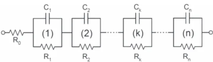
Kramers–Kronig analysis.—The simulated and measured im-pedance data were tested for compliance with the Kramers–Kronig relations using the measurement-model method. The method to assess Kramers–Kronig consistency, developed by Agarwal et al., is based onfitting a measurement model of sequential Voigt elements shown in Fig. 1 to either the real or imaginary component of impedance data and then predicting the other component of impedance from the extracted parameters.43,44As the circuit shown in Fig.1satisfies the Kramers–Kronig relations, the ability to fit the measurement model to experimental data demonstrates consistency of the data to the Kramers–Kronig relations.
An important advantage of the measurement model approach is that it identifies a small set of model structures that are capable of representing a large variety of observed behaviors or responses. The inability tofit an impedance spectrum by a measurement model can be attributed to the failure of the data to conform to the assumptions
of the Kramers–Kronig relations rather than to the failure of the model. The measurement model approach allows calculation of a confidence interval, providing a statistical rigor to the rejection of data due to failure to conform to the Kramers–Kronig relations. A disadvantage of the measurement model approach is that regression is strongly influenced by data outliers.
The experimentally measured impedance data were also tested for Kramers–Kronig compliance by linear measurement model approach developed by Boukamp45 and implemented by Gamry Instruments. In this approach, the Voigt elements arefitted via linear equations to a selected region of the spectrum. Values of time constant t =k 1/R Ck k are specified as the inverse of frequencies
selected over the experimental range of frequencies. This yields a set of linear equations to be solved for values of the corresponding R .k
An advantage of the Boukamp approach is that it is less sensitive to outliers. A disadvantage is that confidence intervals are not provided for the resulting comparison between experiment and measurement model.
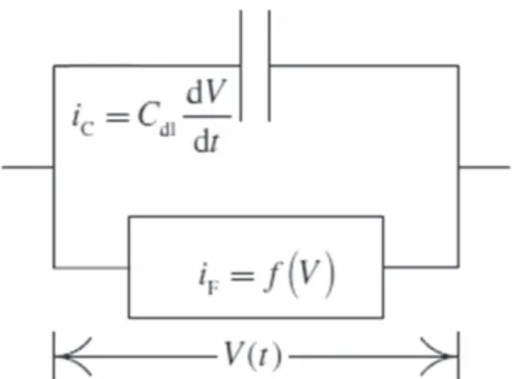
Model system simulation.—The non-stationarity was simulated on a system in which a charging current is added to a faradaic current given by a Tafel expression with a time-dependent rate constant as shown in Fig.2.42The applied potential for the single sine case was a sinusoidal perturbation as
( p ) [ ]
= D
V V sin 2 fi 2
where DV is the input amplitude and fiis the input frequency in the
frequency range of fi = 1 Hz~1 kHzwith 10 points/decade.
The applied potential for the multi-sine case was a sinusoidal perturbation as ⎜ ⎟ ⎛ ⎝ ⎞⎠ ( p j) j p ( ) [ ] = D + = ¼ V V f k N k N sin 2 i i, i 2 1, 2, 3 3 where jiis the phase shift andN=31.
The faradaic current density and the charging current density were expressed as ( ) ( ) [ ] = - -IF Kaexp b Va Kcexp b Vc 4 [ ] = I C V t d d 5 C dl
where ba and bc are the anodic and cathodic coefficients with
= =
-ba bc 19.5 V .1 The values of Ka,Kc were Ka=Kc=0.14´
/
-10 3mA cm2 and the double layer capacitance was C = dl
/ m
31 F cm .2 The impedance response was calculated by a Fourier
analysis for the single-sine potential perturbation and by an FFT analysis for the multi-sine.
The simulation was performed with linear and exponential increases in the charge-transfer resistances which caused a decrease of the rate constant as a function of time. The behavior was expressed as
( g) ( ) ( g) ( ) [ ]
= - - -
-IF Ka 1 exp b Va Kc 1 exp b Vc 6 where g =0.01t for a linear decrease in active area, and
( ( ))
g =0.1 1-exp -t for an exponential decrease in active area. The variation of g used in the simulations is presented in Fig.3. The corresponding charge-transfer resistance increased from 183.2Ω to 203.5Ω within 10 s.
Results
Results are presented for the single-sine and multi-sine impe-dance of a Li\SOCl2 primary battery with a DC offset known to cause nonstationary behavior. Results are also presented for the single-sine and multi-sine impedance of synthetic data designed to represent a nonstationary system. Both the Boukamp45 and the Agarwal et al.43,44methods were used to explore consistency with the Kramers–Kronig relations.
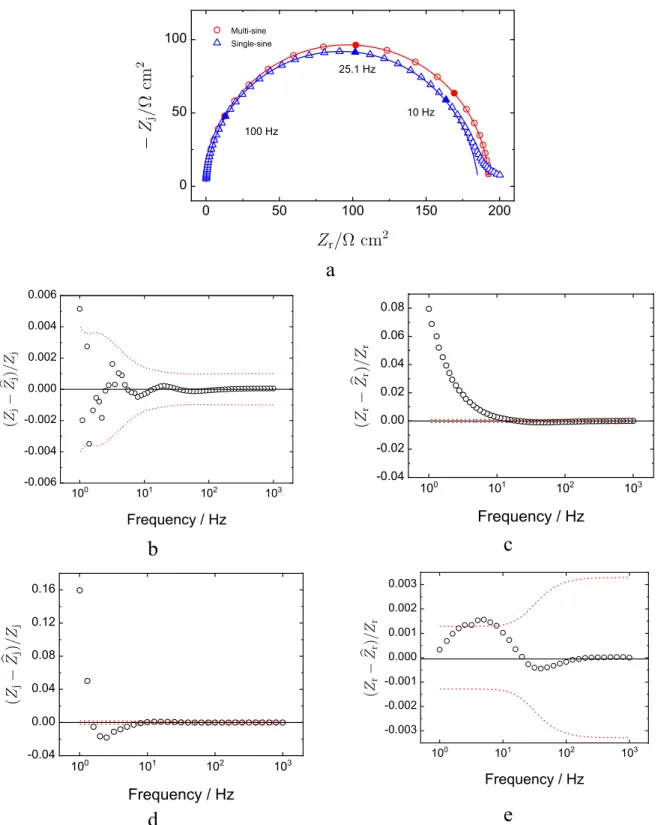
Experimental measurement: Li\SOCl2 with DC offset.—The experimentally measured single-sine and multi-sine impedance of the Li\SOCl2battery under nonstationary conditions are shown in Fig. 4. The lines shown in Fig. 4 are the result of the linear Kramers–Kronig analysis reported by Boukamp44,45 and imple-mented by Gamry. The superposition of the lines with the multi-sine data indicates that the multi-sine data satisfy the Kramers–Kronig relations; whereas, the single-sine data show deviation in the Kramers–Kronig compliance. The deviation is seen most readily in plots of the phase as shown in Fig.4d.
A more sensitive analysis can be obtained by use of the measurement model as developed by Agarwal et al.43,44The results presented in Fig.5reflect the results of a fit of the measurement model to the imaginary part of the impedance for the single-sine data and a complex fit for the multi-sine. For this system, the imaginaryfit yielded more statistically significant parameters for the single-sine data than could be achieved by a complex fit; whereas, the complex fit yielded more statistically significant parameters for the multi-sine data than could be achieved by an imaginaryfit.
As shown in Nyquist format in Fig.5a, the measurement model provided an adequate fit of the single-sine data only at higher frequencies; whereas, the measurement model provided an excellent fit to the multi-sine data over the complete measured range of frequencies. The measurement model provided an excellentfit to the imaginary part of the single-sine data, but the experimental data deviated from the predicted real part of the measurement, as shown in Fig.5d. The complex fit of the measurement model yielded an Figure 2. Circuit representation of the faradaic current and the double layer
capacitor used in the simulation.
Figure 3. Behavior of the fraction of inactive areaγ as a function of time for the calculation of the impedance of nonstationary systems.
excellent agreement to the imaginary (Fig. 5c) and real (Fig. 5e) parts of the measurement.
A more detailed analysis may be obtained by an examination of the residual errors shown in Fig. 6. The residual errors for the regression to the imaginary part of the single-sine measurement are shown in Fig.6a, and the errors in the prediction of the real part of the measurement is shown in Fig. 6b. The large errors at low frequency are consistent with the results presented in Fig. 5a. In contrast, the residual errors for a complexfit to the multi-sine data shown in Fig. 6c and d indicate that the measurement model provided a good fit to the data. The residual errors fall within the 95.4% confidence interval for the model; thus, the data may be considered to be consistent with the Kramers–Kronig relations. A
complexfit to the single-sine data yielded residual errors that were outside the 95.4% confidence interval for the model. This work shows that the single-sine data did not satisfy the Kramers–Kronig relations.
The experimental work presented in Figs.4–6shows that multi-sine method yielded Kramers–Kronig-consistent impedance data for a nonstationary system for which a single-sine approach showed failure to conform to the Kramers–Kronig relations. The time allocated for the multi-sine measurement was 70% larger than the time allocated for the single-sine measurements; thus, the system had ample time to demonstrate nonstationary behavior. The issue is that the presence of nonstationary behavior for a multi-sine measurement could not be identified by application of the Figure 4. Single-sine and multi-sine impedance response for a Li\SOCl2battery under nonstationary conditions: (a) Nyquist; (b) and (c) magnitude for
single-sine and multi-single-sine measurements, respectively; and (d) and (e) phase for single-single-sine and multi-single-sine measurements, respectively. Lines represent the results of a linear Kramers–Kronig analysis as implemented by the Gamry software.
Kramers–Kronig relations. The results suggest also that the mea-surement model implementation by Agarwal et al.43,44 was more sensitive to failures to satisfy the Kramers–Kronig relations than was the linear implementation by Boukamp.45
Numerical simulation: linear increase in charge-transfer re-sistance.—The single-sine and multi-sine calculations were de-signed such that the elapsed times for the simulated impedance measurements were identical. Thus, the level of nonstationarity experienced for the two calculations was the same. The perturbation
amplitude for the single-sine calculations was 1 mV, and the perturbation amplitude for the multi-sine calculations was 0.5 mV. To minimize superposition, the phase angles of signals used to construct the multi-sine potential input were staggered. The effective maximum potential amplitude was 5 mV.
Results are presented in Fig.7for the impedance calculated under the linear transient increase in charge-transfer resistance shown in Fig.3. The Nyquist plots shown in Fig.7a show that, while the single-sine calculations revealed a low-frequency tail corresponding to the increase in charge-transfer resistance, the multi-sine calculations Figure 5. Results of the measurement model analysis of the data presented in Fig. 4: (a) Nyquist; (b) and (c) imaginary for single-sine and multi-sine measurements, respectively; and (d) and (e) real for single-sine and multi-sine measurements, respectively. Solid lines represent the results of a measurement modelfit to the imaginary part of the spectrum for single-sine measurements and both real and imaginary parts of the spectrum for the multi-sine measurements. Dashed lines in b-e represent 95.4% confidence intervals for the model.
produced a semicircle with a radius between the initial and final charge-transfer resistance. Regression of the measurement model to the imaginary part of the single-sine impedance yielded the normal-ized residual error presented in Fig.7b, indicating an excellentfit to the data. The normalized prediction errors for the real part of the measurement, shown in Fig.7c, show that the low-frequency real part of the data was inconsistent with the imaginary part of the data. Thus, the Kramers–Kronig relations were not satisfied for the single-sine simulations.
The residual errors for a complexfit to the multi-sine simulations are presented in Fig.7d and e. These results could befit by only a single RC element. The simulations yielded scatter at low frequency that could be diminished by increasing the elapsed time for the signals. In a purely numerical study, a similar result for synthetic calculations of multi-sine impedance was reported by Srinivasan et al.49 and attributed to failure to satisfy the Kramers–Kronig relations. The Boukamp implementation of the Kramers–Kronig relations, however, showed these simulated data to be consistent. The multi-sine calculation of the impedance yielded a semicircle with scattered values at low frequency. The measurement model analysis reported the charge transfer resistance to be Rt= 193.2 Ω cm2, which was the temporal average. The capacitance was obtained as Cdl= 31 μF cm−2, which was the same as the input.
Numerical simulation: exponential increase in charge-transfer resistance.—Results are presented in Nyquist format in Fig.8a for
the impedance calculated under the exponential transient increase in charge-transfer resistance shown in Fig. 3. The charge-transfer resistance transient was characterized by a rapid increase in resistance at short times at which the singe-sine calculation yielded high-frequency values of the impedance. The shape of the single-sine results reveals that the charge-transfer resistance was almost constant for the calculation of lower frequencies. The single-sine calculations yielded a distorted semicircle; whereas, the multi-sine calculations produced a semicircle with a radius between the initial andfinal charge-transfer resistance. Regression of the measurement model to the imaginary part of the single-sine impedance yielded the normalized residual error presented in Fig. 8b, indicating an excellent fit to the data. The normalized prediction errors for the real part of the measurement, shown in Fig.8c, show that the data were inconsistent with the Kramers–Kronig relations over a broad frequency range. Again, the Kramers–Kronig relations were not satisfied for the single-sine simulations.
The residual errors for a complexfit to the multi-sine simulations, presented in Figs. 8d and e, were similar to those presented in Figs. 7d and e for a linear increase in charge-transfer resistance. Again, these results could befit by only a single RC element. The simulations yielded scatter at low frequency that could be dimin-ished by increasing the elapsed time for the signals. The multi-sine calculation of the impedance yielded a semicircle with scattered values at low frequency. The measurement model analysis showed a value of charge transfer resistance of Rt= 201.38 Ω cm2, which is Figure 6. Normalized residual errors resulting from a measurement modelfit to the data presented in Fig.4: (a) results of a measurement modelfit to the imaginary part of the spectrum for single-sine measurements and (b) the resulting error in the prediction of the real part of the measurement; (c) and (d) imaginary and real residual errors for a complexfit to both real and imaginary parts of the spectrum for the multi-sine measurements. Dashed lines in represent 95.4% confidence intervals for the model.
the temporal average. The capacitance was found as Cdl= 31 μF cm−2which is the same as the input.
Discussion
The experimental and simulation results in the present work demonstrate that the Kramers–Kronig relations do not provide a
means of determining, for multi-sine measurements, whether the system has undergone a transient change during the course of the impedance measurement. The multi-sine technique provides a temporally averaged impedance diagram which satisfies automati-cally the Kramers–Kronig relations. In contrast, application of the Kramers–Kronig relations can reveal nonstationary behavior from single-sine measurements.
Figure 7. Calculated impedance for the linear increase of the charge-transfer resistance for single and multi-sine signals: (a) Nyquist plot for single-sine and multi-sine results with lines representing the correspondingfit of the measurement model; (b) and (c) normalized residual and prediction errors respectively, for a measurement modelfit to the imaginary part of the single-sine impedance; and (d) and (e) normalized residual errors for a complex measurement model fit to multi-sine impedance. Dashed lines in b-e represent 95.4% confidence intervals for the model.
In principle, the coherence function ( ) ∣ ( )∣ ( ) ( ) [ ] w w w w = C P P P 7 xy xy xx yy 2
can provide a means for assessing the quality of input signals used to assess the impedance. In Eq.6, the coherence function Cxyis a real number between 0 and 1 that measures the correlation between the input signal x(t) and the output signal y(t). A value of unity means that the two signals are considered to correspond to each other perfectly at a given frequency. Pxxand Pyyare the power spectra of x (t) and y(t), respectively, and Pxy is the average cross-power spectrum of x(t) and y(t).
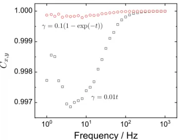
The coherence function calculated for the synthetic multi-sine impedance values presented in Figs.7 and 8varied slightly from unity, as shown in Fig.9. The maximum variation was 0.3% for the linear variation of charge-transfer resistance and 0.02% for the exponential decaying variation of charge-transfer resistance. This level of variation would be masked by experimental artifacts in electrochemical measurements. Further, the coherence calculation suffers from sensitivity to window size and shape selection and artifacts due to timing inaccuracies. Therefore, the coherence function was not explored further for experimental data. On the other hand, inspecting the full Fourier space can be considered to be an alternative for inspecting non-linearity and non-stationarity in multi-sine impedance spectra. Figures10b and10d show the multi-Figure 8. Calculated impedance for the exponential increase of the charge-transfer resistance for single and multi-sine signals: (a) Nyquist plot for single-sine and multi-sine results with lines representing the correspondingfit of the measurement model; (b) and (c) normalized residual and prediction errors respectively, for a measurement modelfit to the imaginary part of the single-sine impedance; and (d) and (e) normalized residual errors for a complex measurement model fit to multi-sine impedance. Dashed lines in b-e represent 95.4% confidence intervals for the model.
sine current excitation and the resulting voltage in the frequency domain for two experiments done with galvanostatic control. These datasets can essentially be read in two parts: the signal and the noise. On the logarithmic y-scale, the points that are high are those frequencies that are excited by the applied signal and the corre-sponding measurement are the signal and the more crowded points that are much lower are the noise level of the applied signal for the excitation and the result of any nonlinearity and drift for the measured signal. The noise floor shown for the voltage signal on the graphs depend on the settings on the instrument, environment noise, etc. As shown in Fig.10b, non-stationarity can be observed in the unexcited frequencies in the frequency domain signal. Non-stationarity exhibits a signal that is below the noise level of the instrument at high frequencies, but gradually increases as the frequency gets lower. It eventually gets above the noise level and keeps rising until the lowest frequency. In contrast for a stationary
system shown in Fig.10d, such behavior is not observed. One way of quantifying the total power at the unexcited frequencies is the so-called“Total Harmonic Distortion (THD)”52–56which is the integral of power in the frequencies that are not excited by the excitation. Though THD provides no distinction between linearity and non-stationarity, it is a good parameter to check for both effects in bulk. The present work provided the opportunity to explore the relative merits of two different implementations of the measurement model for assessing consistency with the Kramers–Kronig relations. The linear regression approach pioneered by Boukamp45allows speci fi-cation of one time constant for every measured frequency, thus providing a point by point analysis that is insensitive to outliers. The point by point analysis is evident in the results for the multi-sine data presented in Fig.4a. In contrast, the analysis pioneered by Agarwal et al.43,44relies on nonlinear regression and can resolve only a small number of parameters. As shown in Figs.5and6, the approach of Agarwal et al.44,45was very sensitive to the failure of the single-sine data to conform to the Kramers–Kronig relations and demonstrated unequivocally the extent to which the multi-sine data satisfied the Kramers–Kronig relations. A more subtle deviation is seen between model and single-sine data in Fig. 4. The Boukamp approach is preferred for data, such as those with outliers, for which an adequate number of RC elements cannot be resolved.
Conclusions
Impedance measurements and model system simulations with single-sine and multi-sine excitations were performed for non-stationary systems. The obtained impedance results were tested for the compliance with Kramers–Kronig relations with measurement model methods. The non-stationary experimental measurements were performed on a Li\SOCl2 primary battery with moderated DC offset. Both nonlinear measurement model and linear measure-ment model methods showed that the obtained impedance spectra with single-sine excitation were inconsistent with Kramers–Kronig relation; whereas, the multi-sine spectra were consistent with the Kramers–Kronig relations. The non-stationarity was simulated with linear and exponential increase in the charge transfer resistance. In both cases the calculated impedance spectra with single-sine signals Figure 9. Coherence function calculated for the multi-sine simulations
presented in Figs.7and8.
Figure 10. Multi-sine impedance response for a Li\SOCl2battery under nonstationary conditions: (a) Nyquist; (b) Frequency domain of the current excitation
and the voltage signals. Multi-sine impedance response for a Dummy Cell in stationary conditions: (c) Nyquist; (d) Frequency domain of the current excitation and the voltage signals.
were found to be inconsistent with the Kramers–Kronig relation. On the other hand, the calculated impedance spectra with multi-sine signals were found to be consistent with the Kramers–Kronig relations.
The present work demonstrates that the validity of multi-sine impedance spectra cannot be assessed by use of the Kramers–Kronig relations. The coherence function, used primarily to detect issues with nonlinear responses, is only modestly sensitive to nonstatio-narity during the course of a multi-sine measurement.
Though the Li\SOCl2battery was used as the sample, the results obtained are universal and the conclusions are relevant well-beyond this sample. In any measurement involving a sample that is not stationary within the timescale of the measurement, a multisine EIS experiment will exhibit data that is compatible with the Kramers–Kronig relations. Therefore, a full Fourier domain analysis is necessary for evaluation using the non-excited frequencies.
Acknowledgments
Mark Orazem acknowledges financial support from the University of Florida Foundation Preeminence and the Dr. and Mrs. Frederick C. Edie term professorships.
References
1. A. Sacco,“Electrochemical impedance spectroscopy: fundamentals and application in dye-sensitized solar cells.”Renew. Sustain. Energy Rev., 79, 814 (2017). 2. X. Yuan, H. Wang, J. Colin Sun, and J. Zhang,“AC impedance technique in PEM
fuel cell diagnosis-A review.”Int. J. Hydrogen Energy, 32, 4365 (2007). 3. F. Huet,“A review of impedance measurements for determination of the
state-of-charge or state-of-health of secondary batteries.”J. Power Sources, 70, 59 (1998). 4. S. S. Zhang, K. Xu, and T. R. Jow,“EIS study on the formation of solid electrolyte
interface in Li-ion battery.”Electrochim. Acta, 51, 1636 (2006).
5. I. A. J. Gordon et al.,“Electrochemical Impedance Spectroscopy response study of a commercial graphite-based negative electrode for Li-ion batteries as function of the cell state of charge and ageing.”Electrochim. Acta, 223, 63 (2017). 6. M. Ates,“Review study of electrochemical impedance spectroscopy and equivalent
electrical circuits of conducting polymers on carbon surfaces.” Prog. Org. Coatings, 71, 1 (2011).
7. E. Cano, D. Lafuente, and D. M. Bastidas,“Use of EIS for the evaluation of the protective properties of coatings for metallic cultural heritage: a review.”J. Solid State Electrochem., 14, 381 (2010).
8. V. M. Huang, S.-L. Wu, M. E. Orazem, N. Pébère, B. Tribollet, and V. Vivier, “Local electrochemical impedance spectroscopy: a review and some recent developments.”Electrochim. Acta, 56, 8048 (2011).
9. T. Muselle, H. Simillion, D. Van Laethem, J. Deconinck, and A. Hubin,“Feasibility study and cell design for performing local electrochemical impedance spectroscopy measurements using an atomic force microscopy set-up.”Electrochim. Acta, 245, 173 (2017).
10. R. Montoya, F. R. García-Galván, A. Jiménez-Morales, and J. C. Galván,“Effect of conductivity and frequency on detection of heterogeneities in solid/liquid interfaces using local electrochemical impedance.”Electrochem. Commun., 15, 5 (2012). 11. M. Mouanga, M. Puiggali, B. Tribollet, V. Vivier, N. Pébère, and O. Devos,
“Galvanic corrosion between zinc and carbon steel investigated by local electro-chemical impedance spectroscopy.”Electrochim. Acta, 88, 6 (2013).
12. C. Gabrielli and M. Keddam,“Review of applications of impedance and noise analysis to uniform and localized corrosion.”Corrosion, 48, 794 (1992). 13. M. A. Zabara, C. B. Uzundal, and B. Ulgut,“Linear and nonlinear electrochemical
impedance spectroscopy studies of Li/SOCl2batteries.”J. Electrochem. Soc., 166, A811 (2019).
14. T. Osaka, D. Mukoyama, and H. Nara,“Review—development of diagnostic process for commercially available batteries, especially lithium ion battery, by electroche-mical impedance spectroscopy.”J. Electrochem. Soc., 162, A2529 (2015). 15. C. Andrade, V. Castelo, C. Alonso, and J. González,“The determination of the
corrosion rate of steel embedded in concrete by the polarization resistance and ac impedance methods.” inCorrosion Effect of Stary Currents and the Techniques for Evaluating Corrosion of Rebars in Concrete (ASTM International, West Conshohocken) p. 43-63 (1986), West Conshohocken, PA: ASTM International0803104685.
16. J. L. Ramirez-Reyes, G. Galicia-Aguilar, J. M. Malo-Tamayo, and J. Uruchurtu-Chavarin, “Electrochemical studies on inorganic zero VOC Coated steel in atmospheric exposure and REAP Test.”ECS Trans., 64, 35 (2015).
17. IviumStat.h standard (accessed November 2, 2019) https://ivium.com/product/ iviumstat-h-standard/.
18. S. C. Creason and D. E. Smith,“Fourier transform faradaic admittance measure-ments. I. Demonstration of the applicability of random and pseudo-random noise as applied potential signals.”J. Electroanal. Chem., 36, A1 (1972).
19. D. E. Smith,“The acquisition of electrochemical response spectra by on-line fast fourier transform: data processing in electrochemistry.”Anal. Chem., 48, 221A (1976).
20. Multisine EIS Implementation: Gamry OptiEIS (accessed November 2, 2019) https://gamry.com/application-notes/EIS/optieis-a-multisine-implementation. 21. Bio-Logic, EIS measurements with multisine (accessed November 2, 2019)https://
bio-logic.net/wp-content/uploads/20101209-Application-note-19.pdf(2010). 22. J. Házì, D. M. Elton, W. A. Czerwinski, J. Schiewe, V. A. Vicente-Beckett, and A.
M. Bond, “Microcomputer-based instrumentation for multi-frequency Fourier transform alternating current (admittance and impedance) voltammetry.” J. Electroanal. Chem., 437, 1 (1997).
23. J.-S. Yoo and S.-M. Park,“An electrochemical impedance measurement technique employing fourier transform.”Anal. Chem., 72, 2035 (2000).
24. J. E. Garland, C. M. Pettit, and D. Roy,“Analysis of experimental constraints and variables for time resolved detection of Fourier transform electrochemical im-pedance spectra.”Electrochim. Acta, 49, 2623 (2004).
25. Y. Van Ingelgem, E. Tourwé, O. Blajiev, R. Pintelon, and A. Hubin,“Advantages of odd random phase multisine electrochemical impedance measurements.” Electroanalysis, 21, 730 (2009).
26. C. J. Yang, Y. Ko, and S. M. Park,“Fourier transform electrochemical impedance spectroscopic studies on anodic reaction of lead.” Electrochim. Acta, 78, 615 (2012).
27. P. Griffiths, “Fourier transform infrared spectrometry.”Science (80-.)., 222, 297 (1983).
28. E. D. Becker and T. C. Farrar,“Fourier Transform Spectroscopy: New methods dramatically improve the sensitivity of infrared and nuclear magnetic resonance spectroscopy.”Science (80-.)., 178, 361 (1972).
29. W. H. Smyrl,“Digital impedance for faradaic analysis.”J. Electrochem. Soc., 132, 1551 (1985).
30. W. H. Smyrl and L. L. Stephenson,“Digital impedance for faradaic analysis III. copper corrosion in oxygenated 0.1N HCl.”J. Electrochem. Soc., 132, 1563 (1985). 31. J. Ühlken, R. Waser, and H. Wiese,“A fourier transform impedance spectrometer using logarithmically spaced time samples.”Berichte der Bunsengesellschaft für Phys. Chemie, 92, 730 (1988).
32. G. S. Popkirov and R. N. Schindler,“A new impedance spectrometer for the investigation of electrochemical systems.”Rev. Sci. Instrum., 63, 5366 (1992). 33. G. S. Popkirov and R. N. Schindler,“Optimization of the perturbation signal for
electrochemical impedance spectroscopy in the time domain.”Rev. Sci. Instrum., 64, 3111 (1993).
34. C. Gabrielli, F. Huet, and M. Keddam,“Comparison of sine wave and white noise analysis for electrochemical impedance measurements.”J. Electroanal. Chem., 335, 33 (1992).
35. E. Van Gheem et al.,“Electrochemical impedance spectroscopy in the presence of non-linear distortions and non-stationary behaviour.”Electrochim. Acta, 49, 4753 (2004).
36. E. Van Gheem et al.,“Electrochemical impedance spectroscopy in the presence of non-linear distortions and non-stationary behaviour: part II. Application to crystal-lographic pitting corrosion of aluminium.”Electrochim. Acta, 51, 1443 (2006). 37. M. Meeusen, P. Visser, L. Fernández Macía, A. Hubin, H. Terryn, and J. M. C. Mol,
“The use of odd random phase electrochemical impedance spectroscopy to study lithium-based corrosion inhibition by active protective coatings.”Electrochim. Acta, 278, 363 (2018).
38. T. Hauffman, Y. van Ingelgem, T. Breugelmans, E. Tourwé, H. Terryn, and A. Hubin,“Dynamic, in situ study of self-assembling organic phosphonic acid monolayers from ethanolic solutions on aluminium oxides by means of odd random phase multisine electrochemical impedance spectroscopy.”Electrochim. Acta, 106, 342 (2013).
39. G. Meyer, H. Ochs, W. Strunz, and J. Vogelsang,“Barrier coatings with high ohmic resistance: comparison between relaxation voltammetry and electrochemical impedance spectrosscopy.”Mater. Sci. Forum, 289–292, 305 (1998).
40. R. Jurczakowski and A. Lasia,“Limitations of the potential step technique to impedance measurements using discrete time fourier transform.”Anal. Chem., 76, 5033 (2004).
41. ZAHNER-Elektrik GmbH & CoKG - Germany, Highend Data Acquisition Systems for Electrochemical Applications ∣ iMSine—Intelligent multi-sine excitation (accessed November 2, 2019) http://zahner.de/support/application-notes/imsine-intelligent-multi-sine-excitation.html.
42. M. E. Orazem and B. Tribollet, in Electrochemical Impedance Spectroscopy. (Wiley, Hoboken, NJ, USA) (2017)9781119363682.
43. P. Agarwal, M. E. Orazem, and L. H. Garcia-Rubio,“Measurement models for electrochemical impedance spectroscopy: I. demonstration of applicability.” J. Electrochem. Soc., 139, 1917 (1992).
44. P. Agarwal, M. E. Orazem, and L. H. Garcia-Rubio,“Application of measurement models to impedance spectroscopy III. evaluation of consistency with the kramers-kronig relations.”J. Electrochem. Soc., 142, 4159 (1995).
45. B. A. Boukamp,“A linear Kronig–Kramers transform test for immittance data validation.”J. Electrochem. Soc., 142, 1885 (1995).
46. S. Real and D. D. Macdonald,“Application of kramers-kronig transforms in the analysis of electrochemical impedance data: II. transformations in the complex plane.”J. Electrochem. Soc., 133, 2018 (1986).
47. B. Hirschorn and M. E. Orazem,“On the sensitivity of the kramers-kronig relations to nonlinear effects in impedance measurements.” J. Electrochem. Soc., 156, C345–51 (2009).
48. M. Urquidi-Macdonald, S. Real, and D. D. Macdonald,“Applications of kramers-kronig transforms in the analysis of electrochemical impedance data-III. Stability and linearity.”Electrochim. Acta, 35, 1559 (1990).
49. R. Srinivasan, V. Ramani, and S. Santhanam,“Multi-Sine EIS-Drift.” Non Linearity and Solution Resistance Effects’, ECS Trans., 45, 37 (2013).
50. R. L. Sacci, F. Seland, and D. A. Harrington,“Dynamic electrochemical impedance spectroscopy, for electrocatalytic reactions.”Electrochim. Acta, 131, 13 (2014). 51. J. R. Macdonald,“Some new directions in impedance spectroscopy data analysis.”
Electrochim. Acta, 38, 1883 (1993).
52. G. S. Popkirov and R. N. Schindler,“A new approach to the problem of ‘good’ and ‘bad’ impedance data in electrochemical impedance spectroscopy.”Electrochim. Acta, 39, 2025 (1994).
53. J. J. Giner-Sanz, E. M. Ortega, and V. Pérez-Herranz,“Total harmonic distortion based method for linearity assessment in electrochemical systems in the context of EIS.”Electrochim. Acta, 186, 598 (2015).
54. J. J. Giner-Sanz, E. M. Ortega, and V. Pérez-Herranz, “Optimization of the perturbation amplitude for EIS measurements using a total harmonic distortion based method.”J. Electrochem. Soc., 165, E488 (2018).
55. Total Harmonic Distortion: Theory and Practice (accessed November 2, 2019) https://gamry.com/application-notes/EIS/total-harmonic-distortion/.
56. THD: parameters affecting its value and comparison with other methods of linearity assessment (accessed November 2, 2019)https://bio-logic.net/wp-content/uploads/ AN65_more_details_on-THD.pdf.
57. D. D. Macdonald, “Reflections on the history of electrochemical impedance spectroscopy.”Electrochim. Acta, 51, 1376 (2006).