THE BEHAVIOR OF TRANSIENT PERIOD OF
NONTERMINATING SIMULATIONS:
AN EXPERIMENTAL ANALYSIS
A THESIS
SUBMITTED TO THE DEPARTMENT OF INDUSTRIAL ENGINEERING AND THE INSTITUTE OF ENGINEERING AND SCIENCES
OF BİLKENT UNIVESITY
IN PARTIAL FULFILLMENT OF THE REQUIREMENTS FOR THE DEGREE OF
MASTER OF SCIENCE
By
Burhaneddin Sandıkçı August, 2001
ii
I certify that I have read this thesis and that in my opinion it is fully adequate, in scope and in quality, as a thesis of the degree of Master of Science
Assoc. Prof. İhsan Sabuncuoğlu (Principal Advisor)
I certify that I have read this thesis and that in my opinion it is fully adequate, in scope and in quality, as a thesis of the degree of Master of Science
Asst. Prof. Oya Ekin Karaşan
I certify that I have read this thesis and that in my opinion it is fully adequate, in scope and in quality, as a thesis of the degree of Master of Science
Asst. Prof. Yavuz Günalay
Approved for the Institute of Engineering and Sciences
Prof. Dr. Mehmet Baray
ABSTRACT
The design and control of many industrial and service systems require the analysts to account for uncertainty. Computer simulation is a frequently used technique for analyzing uncertain (or stochastic) systems. One disadvantage of simulation modeling is that simulation results are only estimates of model performance measures. Therefore, to obtain better estimates, the outputs of a simulation run should undergo a careful statistical analysis. Simulation studies can be classified as terminating and nonterminating according to the output analysis techniques used. One of the major problems in the output analysis of nonterminating simulations is the problem of initial transient. This problem arises due to initializing simulation runs in an unrepresentative state of the steady-state conditions.
Many techniques have been proposed in the literature to deal with the problem of initial transient. However, existing studies try to improve the efficiency and effectiveness of currently proposed techniques. No research has been encountered that analyzes the behavior of the transient period. In this thesis, we investigate the factors affecting the length of the transient period for nonterminating manufacturing simulations, particularly for serial production lines and job-shop production systems. Factors such as variability of processing times, system size, existence of bottleneck, reliability of system, system load level, and buffer capacity are investigated.
Keywords: Nonterminating simulations, behavior of transient period, serial production
ÖZET
Birçok endüstriyel ve servis sisteminin tasarım ve kontrolü için analizi yapan kimselerin berlirsizliği hesaba katlamaları gerekir. Bilgisayar benzetim tekniği belirsiz (veya rassal) sistemlerin analizinde sıkça kullanılan bir yöntemdir. Benzetim modellerinin önemli bir eksiği performans değerleri için sadece tahminler üretmesidir. Bu nedenle, daha doğru sonuçlar elde edebilmek için benzetim çıktıları dikkatli istatistiki analize tabi tutulmalıdır. Benzetim çalışmaları, kullanılan çıktı analizi tekniklerine göre sonu belirli ve sonu belirsiz olarak sınıflandırılabilirler. Sonu belirsiz benzetimlerin çıktı analizinde karşılaşılan en önemli problemlerden biri geçiş dönemi problemidir. Bu problem benzetim modelini uzun vadedeki durumundan uzak bir konumda başlatmaktan ötürü ortaya çıkar.
Başlangıçtaki geçiş dönemi probleminin çözümüne dair önerilmiş pekçok teknik literatürde mevcuttur. Fakat mevcut çalışmalar daha çok önerilen tekniklerin etkinlik ve yeterliliğini geliştirmeye çalışmaktadır. Geçiş döneminin davranışını inceleyen bir çalışma ile karşılaşılmamıştır. Biz bu tezde, sonu belirsiz benzetimlerle analiz edilen imalat sistemlerinin geçiş dönemini etkileyen faktörleri inceliyoruz. Özellikle seri üretim hatları ve atölye sistemleri üzerinde duruyoruz. İşlem zamanının değişkenliği, sistemin büyüklüğü, darboğazın mevcudiyeti, sistemin güvenilirliği, sistemin yük seviyesi ve tamponların kapasitesi incelenen faktörler arasındadır.
Anahtar Sözcükler: Sonu belirsiz benzetim, geçiş dönemi davranışı, seri üretim hatları,
ACKNOWLEDGEMENTS
When I approached the near end, I recognized that it was not a so long journey. However, while I was in the middle of this suffering process, it seemed to be never ending. Thanks God for the knowledge, patience, and power He gave to me to finish this and all other tasks.
I would like to express my sincere gratitude to Assoc. Prof. İhsan Sabuncuoğlu for his supervision and encouragement during my graduate study. His trust and understanding motivated me and let this thesis come to an end.
I am indebted to Asst. Prof. Oya Ekin Karaşan for her invaluable support during my first year at Bilkent University. I owe so much to her for her interest and encouragement. I also would like to thank her for reading and reviewing this thesis.
I am greateful to Asst. Prof. Yavuz Günalay for accepting to read and review this thesis and for his suggestions.
I am so much indebted to Prof. Kemal Sandıkçı for all his invaluable teachings and for introducing me to the One upon whom the universe is created for. I also would like to thank to Prof. Erkan Türe for his never ending morale support during all my studies. Special thanks goes to Prof. K. Preston White for his technical support about MSER heuristics.
I have so much enjoyed meeting Abdullah Karaman and he deserves very special thanks for being a so good friend. Thanks to Mustafa Akbas for his technical help and patience. I also would like thank Çağrı Gürbüz, Onur Boyabatlı, Savaş Çevik, Rabia Köylü, Ayten Türkcan, Banu Yüksel, Erkan Köse, and Hüseyin Karakuş for their friendship.
Ali Kasap, Erkan Sarıkaya, Murat Ay, Ersin Yurdakul, Berkant Çamdereli, and Almula Şahin all shared my troubles and helped me in those days. I would not be in my current situation without their guidance.
Finally, I would like to express my deepest gratitude to Zahide Yavuz for her patience, understanding, kindness, and the happiness she brought to my life.
Contents
1 INTRODUCTION... 1
The need for modeling ... 1
Simulation modeling... 2
The need for analysis of simulation outputs ... 3
The problem of initial transient in simulation outputs ... 4
Motivation of the proposed study ... 5
2 THE PROBLEM OF INITIAL TRANSIENT... 7
2.1 INTRODUCTION... 7
2.2 BASIC STATISTICAL CONCEPTS... 8
Case 1. Independent and identically distributed sequences ... 8
Case 2. Correlated sequences ... 10
2.3 THE BEHAVIOR OF SIMULATION OUTPUTS AND ANALYSIS METHODS... 13
Method of independent replications ... 18
2.4 PROBLEM DEFINITION... 20
Mitigating the effects of initialization bias ... 22
2.5 LITERATURE SURVEY... 23
2.6 DATA TRUNCATION TECHNIQUES TO REDUCE INITIALIZATION BIAS... 30
Plotting the cumulative average graph ... 33
3 THE PROPOSED STUDY... 37
3.1 THE METHODOLOGY USED IN THIS STUDY... 38
3.2 AN EXAMPLE... 47
3.3 SYSTEM CONSIDERATIONS AND EXPERIMENTAL DESIGN... 52
4 RESULTS FOR SERIAL PRODUCTION LINES ... 59
The structural framework in the presentation of outputs ... 60
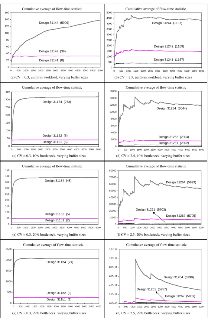
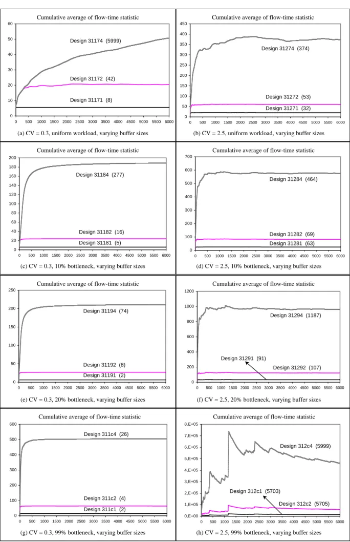
4.1 THE EFFECT OF BUFFER CAPACITY... 61
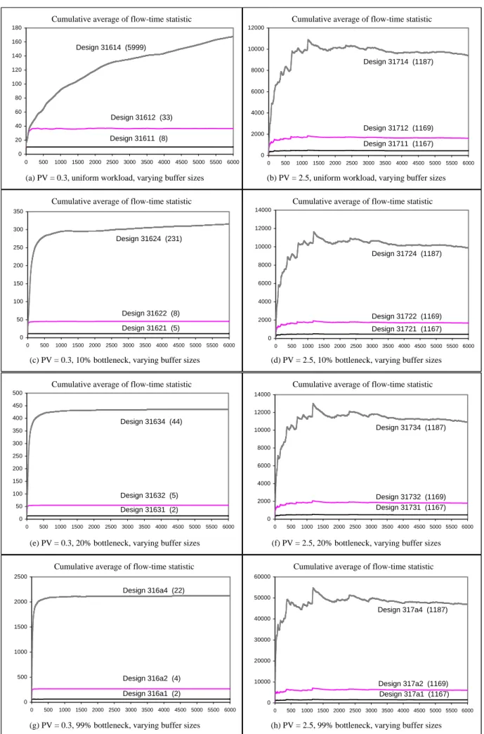
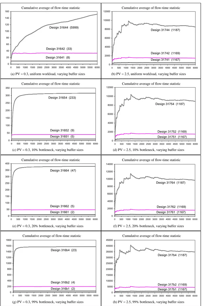
4.2 THE EFFECT OF PROCESSING TIME VARIABILITY... 62
4.3 THE EFFECT OF LINE LENGTH... 64
4.4 THE EFFECT OF DISTRIBUTION OF SYSTEM LOAD... 65
4.5 THE EFFECT OF SYSTEM LOAD LEVEL... 67
4.6 THE EFFECT OF RELIABILITY... 70
4.7 THE EFFECT OF UTILIZATION... 73
5 RESULTS FOR JOB-SHOP PRODUCTION SYSTEMS ... 94
The structural framework in the presentation of outputs ... 94
5.1 THE EFFECT OF PROCESSING TIME VARIABILITY... 96
5.2 THE EFFECT OF SYSTEM SIZE... 97
5.3 THE EFFECT OF DISTRIBUTION OF SYSTEM LOAD... 97
5.4 THE EFFECT OF SYSTEM LOAD LEVEL... 99
5.5 THE EFFECT OF RELIABILITY... 101
5.6 THE EFFECT FINITE BUFFER CAPACITIES... 101
6 CONCLUSIONS ... 111
REFERENCES ... 117
APPENDIX A. RANDOM NUMBER STREAMS... 126
APPENDIX B. BREAKDOWN PARAMETERS ... 128
APPENDIX D. SUMMARY STATISTICS... 135
APPENDIX E. SAME SCALE FIGURES ... 146
APPENDIX F. SAMPLE INDIVIDUAL PLOTS ... 161
List of Figures
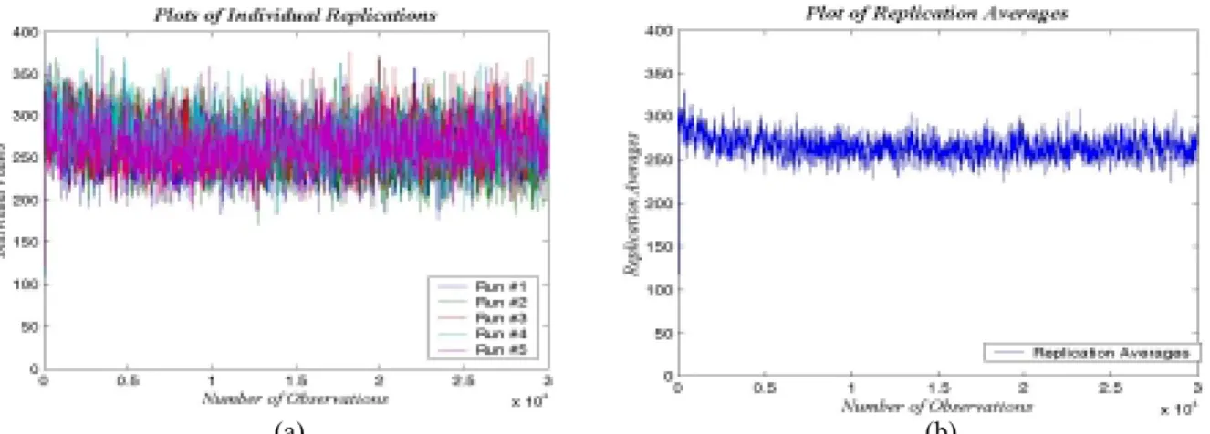
Figure 3.1 Effect of averaging across several replications on the variability of the process...44
Figure 3.2 A plot of the replication averages without deleting outliers...48
Figure 3.3 A plot of the replication averages with deleting outliers...48
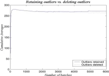
Figure 3.4 Cumulative averages plot for the outliers retained and deleted sequences ...49
Figure 3.5 Effect of outliers in MSER calculations...50
Figure 3.6 The behavior of standard error statistic...50
Figure 3.7 A schematic view of N-staged serial production line...52
Figure 3.8 A schematic view of N-machine job-shop production system. ...53
Figure 4.1 Experimental results for 3-stage serial line containing all reliable machines with a total processing time of 3 minutes per job ...75
Figure 4.2 Experimental results for 3-stage serial line containing all reliable machines with a total processing time of 2.7 minutes per job ...76
Figure 4.3 Experimental results for 3-stage serial line containing all reliable machines with a total processing time of 1.5 minutes per job……….77
Figure 4.4 Experimental results for 3-stage serial line containing all reliable machines with a total processing time of 3 minutes per job ...78
Figure 4.5 Experimental results for 3-stage serial line containing all reliable machines with a total processing time of 2.7 minutes per job ...79
Figure 4.6 Experimental results for 3-stage serial line containing all reliable machines with a total processing time of 1.5 minutes per job ...80
Figure 4.7 Experimental results for 3-stage serial line containing 90% unreliable machines with frequent breakdowns/short repair times and a total processing time of 3 minutes per job ...81
Figure 4.8 Experimental results for 3-stage serial line containing 90% unreliable machines with frequent breakdowns/short repair times and a total processing time of 2.7 minutes per job ...82
Figure 4.9 Experimental results for 3-stage serial line containing 90% unreliable machines with frequent breakdowns/short repair times and a total processing time of
1.5 minutes per job ...83 Figure 4.10 Experimental results for 3-stage serial line containing 90% unreliable machines
with frequent breakdowns/short repair times and a total processing time of
3 minutes per job...84 Figure 4.11 Experimental results for 3-stage serial line containing 90% unreliable machines
with frequent breakdowns/short repair times and a total processing time of
2.7 minutes per job...85 Figure 4.12 Experimental results for 3-stage serial line containing 90% unreliable machines
with frequent breakdowns/short repair times and a total processing time of
1.5 minutes per job...86 Figure 4.13 Experimental results for 3-stage serial line containing 90% unreliable machines
with rare breakdowns/long repair times and a total processing time of
3 minutes per job...87 Figure 4.14 Experimental results for 3-stage serial line containing 80% unreliable machines
with frequent breakdowns/short repair times and a total processing time of
3 minutes per job...88 Figure 4.15 Experimental results for 3-stage serial line containing 50% unreliable machines
with frequent breakdowns/short repair times and a total processing time of
3 minutes per job...88 Figure 4.16 Experimental results for 3-stage serial line containing 80% unreliable machines
with rare breakdowns/long repair times and a total processing time of
3 minutes per job...89 Figure 4.17 Experimental results for 3-stage serial line containing 50% unreliable machines
with rare breakdowns/long repair times and a total processing time of
3 minutes per job...89 Figure 4.18 Experimental results for 9-stage serial line containing all reliable machines
with a total processing time of 9 minutes per job ...90 Figure 4.19 Experimental results for 9-stage serial line containing 90% unreliable machines
with rare breakdowns/long repair times and a total processing time of
9 minutes per job...91 Figure 4.20 Number of jobs in system for 3-stage reliable serial line...92 Figure 4.21 Cumulative averages plot of number in system for 3-stage serial line...92
Figure 4.22 Determining the length of transient period using Welch's technique
for design 91122. ...93 Figure 5.1 Experimental results for 3-machine job-shop containing all reliable machines
with a total processing time of 3 minutes per job ...101 Figure 5.2 Experimental results for 3-machine job-shop containing all reliable machines
with a total processing time of 3 minutes per job ...102 Figure 5.3 Experimental results for 3-machine job-shop containing 90% unreliable machines
with frequent breakdown/short repair times and a total processing time of
3 minutes per job ...103 Figure 5.4 Experimental results for 3-machine job-shop containing 90% unreliable machines
with frequent breakdown/short repair times and a total processing time of
3 minutes per job ...104 Figure 5.5 Experimental results for 3-machine job-shop containing 90% unreliable machines
with rare breakdown/long repair times and a total processing time of
3 minutes per job ...105 Figure 5.6 Experimental results for 3-machine job-shop containing 90% unreliable machines
with rare breakdown/long repair times and a total processing time of
3 minutes per job ...106 Figure 5.7 Experimental results for 9-machine job-shop containing all reliable machines
with a total processing time of 9 minutes per job ...107 Figure 5.8 Experimental results for 9-machine job-shop containing 90% unreliable machines
with frequent breakdown/short repair times and a total processing time of
9 minutes per job ...107 Figure 5.9 Experimental results for 9-machine job-shop containing 90% unreliable machines
with rare breakdown/long repair times and a total processing time of
9 minutes per job ...107 Figure 5.10 Experimental results for 3-machine job-shop containing all reliable machines
List of Tables
Table 2.1 Typical simulation output using method of independent replications ...18
Table 2.2 Summary of the literature on the initial transient problem ...24
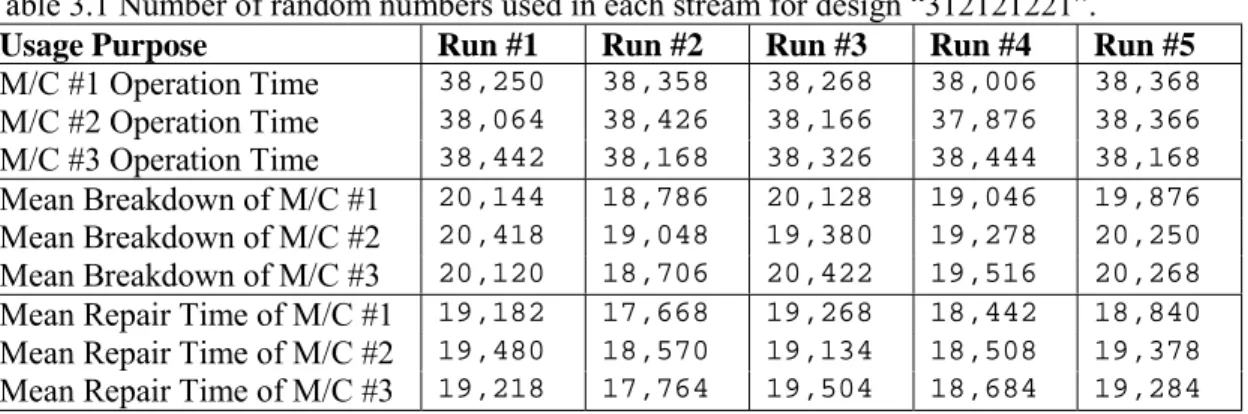
Table 3.1 Number of random numbers used in each stream for design “312121221” ...40
Table 3.2 The format of outputs for a particular model ...41
Table 3.3 Effect of common random numbers (CRN) and independent replications...42
Table 3.4 An example output ...47
Table 3.5 Experimental factors and their levels for serial line system ...55
Table 3.6 Experimental factors and their levels for job-shop system ...55
Table 3.7 Differentiating between constant PV and constant CV...57
Table 3.8 Different breakdown scenarios ...58
Table 4.1 Effect of utilization on the length of the transient period ...73
Table 5.1 Comparison of the variability of low and highly loaded designs...100
Table 6.1 Summary of the results for serial production lines ...112
Table 6.2 Summary of the results for job-shop production systems...112
Table A.1 Usage purpose of different random number streams and their reference points in serial production line experiments...126
Table A.2 Usage purpose of different random number streams and their reference points in job-shop experiments...127
Table B.1 Parameter selection for downtime and uptime distributions ...129
Table C.1 Designs for serial line experiments ...130
Table C.2 Designs for job-shop experiments ...134
Table C.3 Unreliable design names for both serial and job-shop experiments...134
Table D.1 Summary statistics for serial line experiments...135
1 INTRODUCTION
The need for modeling
The idea of conceptualization and modeling plays a crucial role in our understanding of our environment. The modeling concept is often used to represent and express ideas and objects.
A model is defined as a representation of a system for the purpose of studying the system. In other words, models are used because there is a need for learning something about a system, such as relationships among various components, or performance under some specified conditions, which cannot be observed or experimented directly either due to non-existence of the system or difficulty in manipulation of the system. A carefully built model can throw away the complexity and leave only the necessary parts that an analyst is looking for.
The word “system” comprises the vital part of the definition of a model. A system is defined as a group of objects that are joined together in some regular interaction or interdependence toward the accomplishment of some purpose (Banks et al., 1996). The relationships among these objects and the manner in which they interact determine how the system behaves and how well it fulfills its overall purpose. If it is possible and cost-effective to alter the system physically, then it is probably desirable to do so rather than working with a model. However, it is rarely feasible to do this, because such
experimentation would often be too costly or too disruptive to the system. Moreover, the system might not even exist, but it can be of interest to study it in its various proposed alternative configurations to see how it should be built in the first place. For these reasons, it is usually necessary to build a model as a representation of the system and study it as a surrogate for the actual system.
Simulation modeling
Various kinds of models can be built to study systems, where our focus is only on mathematical models. Mathematical models represent a system in terms of logical and quantitative relationships. Mathematical models can be grouped into two categories, namely, analytical models and simulation models. Analytical models make use of mathematical methods, such as algebra, calculus, or probability theory, which obtain exact information on the questions of interest. On the other hand, simulation models evaluate a system numerically and produce only estimates of the true characteristics of the system.
A formal definition of simulation by Fishman (1978) is given as follows: “Simulation is the creation of a model that imitates the behavior of a system, running the model to generate observations of this behavior, and analyzing the observations to understand and summarize this behavior.”
If the model, hence the system is simple enough, then analytical solutions may be possible. If an analytical solution to a model is possible and computationally efficient, it is usually desirable to study the model in this way rather than via a simulation. However, most real-world systems are too complex to allow realistic models to be evaluated analytically, and simulation takes the first place.
Simulation models can be static or dynamic according to the involvement of the passage of time. Another classification of simulation models is on the basis of the characteristics of the input components. If all the inputs are constants than it is called deterministic simulation, whereas a model that contains at least one random input is called stochastic simulation. Stochastic simulation models produce output that is itself random, and therefore must be treated only as an estimate of the true characteristic of the
model. A further classification can be made with regard to the occurrence of events. A discrete-event simulation concerns the modeling of a system as it evolves over time by a representation in which the state variables change instantaneously at separate points in time. A continuous simulation concerns the modeling of a system over time by a representation in which the state variables change continuously with respect to time (Law and Kelton, 2000). In this study, we build discrete, dynamic, and stochastic models. The steps needed for successful application of a simulation study, and advantages/disadvanta-ges of simulation are discussed well in Banks et al. (1996) and Law and Kelton (2000).
There are many application areas of simulation where it is used extensively in the design and analysis of manufacturing systems due to the high degree of complexity. In this thesis, we will focus only on manufacturing system simulations, particularly, serial production lines and job-shop production systems. Other application areas are well listed in Banks et al. (1996) and Winter Simulation Conference (WSC) proceedings are good sources to find interesting applications.
The need for analysis of simulation outputs
From the definition of simulation given above, it can be seen that simulation is just a computerized experiment of a model. Since random samples from probability distributions are typically used as inputs to simulation experiments, the outputs of the experiments will clearly be random variables, too. And the outputs (or estimates) are just particular realizations of random variables that may have large variances. As a result, these estimates could, in a particular run, differ greatly from the corresponding true characteristics of the model. Therefore, there may be a significant probability of making faulty inferences about the system under study. In order to correctly interpret the results of such an experiment, it is necessary to use appropriate statistical analysis tools.
Two crucial problems with an output sequence obtained from a single simulation run are the nonstationarity and the autocorrelation. Nonstationarity means that the distributions of the successive observations change over time, whereas autocorrelation means the observations in the sequence are correlated with each other. Unless carefully analyzed, these two problems may lead the analyst to wrong conclusions.
The problem of initial transient in simulation outputs
Simulation experiments can be classified as either terminating or nonterminating when the output analysis methods are concerned (Law and Kelton, 2000; Fishman, 1978). A terminating simulation is the one for which the starting and stopping conditions are determined a priori by reasoning from the underlying system. Although the starting and stopping conditions are determined by the analyst, which in fact is decided by the nature of the underlying system, these conditions need not only be deterministic but they can very well be stochastic, as well. Since starting and stopping conditions are part of the terminating simulations, relatively straightforward techniques can be used to estimate the parameters of interest in these experiments (e.g., method of independent replications.)
A nonterminating simulation, on the other hand, is the one for which there is no natural starting and stopping conditions. And the aim of a nonterminating simulation is to estimate the parameter of a steady-state distribution. An important characteristic of nonterminating simulations is that steady-state parameter of interest does not depend on the initial conditions of the simulation. However, steady-state exists only in the limit, that is, as the run length goes to infinity. And the run length of any simulation needs to be finite. Therefore, the initial conditions, which normally may not represent the system conditions in the steady-state, will apparently bias the estimates based on the simulation. This is called the problem of initial transient in the simulation literature. Many techniques have been proposed in the literature to remedy this problem (see, for example, Kelton, 1989; Kelton and Law, 1983; Schruben, 1981; Schruben et al., 1983; Goldsman et al., 1994; Vassilacopoulos, 1989; Welch, 1982; and White, 1997; among many others).
The initial transient problem deserves particular attention in any successful simulation study. Almost all of the studies in the literature are in the form of either method developments that try to mitigate the effects of initialization bias or works that compare the effectiveness of proposed techniques via applying them to analytically tractable models. That is, the studies done so far try to assess and improve the efficiency and efficacy of the earlier proposed techniques. We have never seen a study explicitly investigating how the initial transient period behaves with respect to different system conditions. We, in this thesis, are primarily interested in the behavior of the initial
transient. More specifically, we are trying to observe the change in the length of the transient period of nonterminating simulations with changes in the system parameters.
Motivation of the proposed study
The primary motivation for this study comes from the often negligence of initial transient problem in practice, especially when using method of independent replications, and, more importantly, from non-existence of objective procedures to deal with this problem that are guaranteed to work well in every situation. In practice, most practitioners and even academic researchers, as well, often neglect the bias induced by the initial transient period in doing their simulation studies. The analysts, in general, truncate some initial portion of the whole sequence to mitigate the effects of initialization bias, however, they do this truncation in a rather informal way.
Furthermore, in comparing several alternative system designs, the truncation point is chosen by observing only one particular design, which may have a relatively short transient period, and the same amount of data is truncated from all other designs. This strategy, apparently, will not mitigate the effects of bias induced by initial conditions, if some designs have longer transient periods. In making unbiased comparisons among alternative designs, deleting the same amount of data from each design makes sense. However, the length of the transient period, i.e., the number of data to be truncated, might change drastically from one design to the other. Hence, if the same amount of truncation is to be made, then this should be chosen by selecting the longest transient period.
Initialization bias induces more severe problems in the simulation results if the output analysis has to be done by the method of independent replications, which is often the case due to its simplicity. Moreover, there is no objective criterion for data truncation that works well in every situation, which makes the problem even harder. This is, perhaps, one of the main reasons for its negligence. If some guidelines can be given by the researchers about the behavior of the transient period with respect to different system parameters, then the problem discussed above about the comparison of several system designs would be minimized, if not completely eliminated.
For the time being, we restrict our attention only to manufacturing systems, particularly serial production lines and job-shop production systems. The reason for choosing serial production lines and job-shop systems is that they are the building blocks of most manufacturing systems, and one can observe the simplest form of interactions among system components, which than can be generalized to larger systems. Additionally, these systems are of economic importance as they are still the most widely used ones in practical manufacturing. The contribution of this study to the literature can be stated as follows:
• It provides an extensive review of the literature on initial transient problem, which might be a starting point for future research in this area.
• It applies a relatively new truncation technique in addition to a frequently used visual tool, which allows us to assess its applicability in real-world system simulations, to discuss its theoretical limitations, and to give guidelines for its implementation.
• By giving detailed results for manufacturing systems, it provides a framework for simulation practitioners to validate their model findings regarding the transient period, a problem which has not received enough attention.
The organization of the thesis is as follows: after a short introduction to the initial transient problem in Chapter 1, it continues with presenting basic statistical results for the analysis of simulation outputs in Chapter 2. It then continues with a more precise definition of the problem of initial transient, which is followed by a literature survey. After giving some of the solution techniques to the problem of initial transient the chapter ends with a summary. We present the proposed study and the methodology used for this purpose in Chapter 3. Also, the methodology is illustrated by a detailed example. This chapter also discusses the system considerations and experimental parameters that are used in this study. Chapters 4 and 5 present the results of experiments for serial and job-shop production systems, respectively. This thesis ends with a conclusion chapter in which the results of the previous sections are summarized and future research directions are elaborated.
2 THE PROBLEM OF INITIAL TRANSIENT
2.1 Introduction
In this chapter, we study the problem of initial transient in more detail. The inherent variability in simulation data necessitates the use of statistical techniques to have meaningful conclusions from the simulation results. Unless appropriate statistical techniques are used to make the analysis, the results of a simulation experiment are always subject to suspect.
A classification of simulation studies based on the output analysis methods is made as either terminating or nonterminating (Law and Kelton, 2000; and Fishman, 1978). The starting and stopping conditions in a terminating simulation are in the nature of the system; hence the analyst has no control over it. Thus, by making several independent replications of the model one can use classical statistical techniques to analyze the output of terminating simulations. There is no natural starting and stopping conditions for the nonterminating simulations, hence both the way of starting and stopping do affect the performance measures to be estimated by these experiments. This problem should be remedied by careful statistical analysis instead of directly applying the classical methods. In the literature of initial transient problem, almost all the authors try
to improve the efficiency and efficacy of the solution techniques proposed. We, in this study, primarily focus on the behavior of the initial transient (warm-up or start-up) period. We are interested in observing this behavior in the simulation of manufacturing systems, particularly in serial production lines and job-shop production systems. The reason for choosing these systems is that, they are the basic building blocks of more complex manufacturing systems. Additionally, the simplest forms of interaction among system entities can be observed easily, which than can aid to understand the behavior of larger systems.
One can skip Sections 2.2, 2.3, and 2.4 if s/he has enough statistical background and knowledge about the initial transient problem in simulation literature. Specifically, in Section 2.2 we present the basic results, such as calculation of the mean, variance, and confidence interval, from statistical theory. Then, we describe the behavior of a typical simulation output and define the initial transient problem in more precise terms in Sections 2.3 and 2.4, respectively. They are followed, in Section 2.5, by a presentation of the literature done so far on the initial transient problem. The chapter ends with presenting two of the data truncation techniques proposed in the literature in Section 2.6, which are used in this study.
2.2 Basic statistical concepts
Case 1. Independent and identically distributed sequences
Estimating a population mean from a sample data is a common objective of the statistical analysis of a simulation experiment. The mean is a measure of the central tendency of a stochastic process. The median is an alternative measure of the central tendency. In the cases when the process can take on very large and very small values, the median can be a better measure than the mean, since extreme values can greatly affect the mean. However, almost all the studies in the simulation literature deal with the mean rather than the median. Hence, in this study we will not use median, but mean instead.
By estimating the population mean we obtain a single number that serves as the best candidate for the unknown performance parameter. Although this single number, i.e.,
the point estimate, is important, it should always be accompanied by a measure of error. This is usually done by constructing a confidence interval for the performance measure of interest, which is helpful in assessing how well the sample mean represents the population mean. The first step in doing this is to estimate the variance of the point estimator. The variance is a measure of the dispersion of the random variable about its mean. The larger the variance, the more likely the random variable is to take values far from its mean.
Now, suppose that we have a stochastic sequence of n numbers, X1, X2,…, Xn. Further suppose that, this sequence is formed by independent and identically distributed random variables having finite mean μ and finite variance σ2. Independence means that there is no correlation between any pairs in the sequence. Identically distributed means that all the numbers in the sequence come from the same distribution. Then, an unbiased point estimator for the population mean, μ, is the sample mean, X , that is E
[ ]
X =µ , where∑
= = n i i X n X 1 1 (2.1) An unbiased estimator of the population variance, σ2, is the sample variance, S2, that is E[ ]
S2 =σ2, where(
)
∑
= − − = n i i X X n S 1 2 2 1 1 (2.2) Now, due to independence, the variance of the point estimator, Var[ ]
X , can be written as:[ ]
(
)
. ) 1 ( 1 1 2 2∑
= − − = = n i i X X n n n S X Var (2.3)The bigger the sample size n, the closer X should be to μ.
If n is sufficiently large, then an approximate 100(1-α) percent confidence interval for μ is given by ] [ 2 / 1 Var X z X ± −α (2.4)
Law and Kelton (2000) explain this confidence interval as follows: if a large number of independent 100(1-α) percent confidence intervals each based on n
observations are constructed, the proportion of these confidence intervals that contain (cover) μ should be 1-α. However, the confidence interval given by (2.4) holds only when the distribution of X can be approximated by a normal distribution, that is for sufficiently large n. If n is chosen too small, the actual coverage of the desired 100(1-α) percent confidence interval will generally be less than 1-α. To remedy this problem, z-distribution can be replaced by a t-z-distribution.
] [ 2 / 1 , 1 Var X t X ± n− −α (2.5)
Since tn-1,1-α/2 > z1-α/2, the confidence interval given by (2.5) will be larger than the one given by (2.4) and will generally have coverage closer to the desired level 1-α (Law and Kelton, 2000).
Case 2. Correlated sequences
It is important to notice that the results presented so far are valid only if the assumptions of independence and identical distribution holds. If any of these assumptions is violated, then the results might change drastically. Now, we will examine the results when the assumption of independence is violated. We start with a definition of the covariance and correlation.
Let X and Y be two random variables, and let μX = E[X], μY = E[Y], σ2X = Var[X], and σ2Y = Var[Y]. The covariance and correlation are measures of the linear dependence between X and Y. The covariance between X and Y is defined as (Fishman, 1973b);
Cov[X, Y] = E[(X- μX)·( Y- μY)] = E[X·Y] - μX ·μY (2.6) The covariance can take on values between -∞ and ∞. The correlation coefficient, ρ, standardizes the covariance between –1 and 1.
[ ]
Y X Y X Cov σ σ ρ = , (2.7)If ρ is close to +1, then X and Y are highly positively correlated. On the other hand, if ρ is close to –1, then X and Y are highly negatively correlated. The closer ρ is to zero in both sides, the more independence between X and Y.
Now, suppose that we have a sequence of random variables X1, X2,… that are identically distributed but may be dependent. In such a time-series data, we can speak of lag-j autocorrelation.
ρj = ρ (Xi, Xi+j) (2.8)
This means that the value of the autocorrelation depends only on the number of observations between Xi and Xi+j, not on the actual time values of Xi and Xi+j. If the Xi’s are independent , then they are uncorrelated, and thus ρj = 0 for j = 1, 2,… .
When we have an autocorrelated sequence X1, X2, …, Xn, the sample mean, X , given by (2.1) is still an unbiased estimator of the population mean, μ. However, the estimation of the variance of the point estimate becomes a hard job (Banks et al., 1996);
[ ]
∑∑
(
)
= = = n i n j j i X X Cov n X Var 1 1 2 , 1 (2.9) Obtaining the above estimate is certainly a hard job since each term Cov(Xi, Xj) may be different, in general. Fortunately, systems that have a steady-state will produce an output process that is approximately covariance-stationary (Law and Kelton, 2000). If a time-series is covariance-stationary, then the statement given in (2.9) can be simplified to (Moran 1959; Anderson, 1971):[ ]
(
)
− + =∑
− = 1 1 2 1 2 1 n j j n j n S X Var ρ (2.10)It can be shown (see, Law, 1977) that the expected value of the variance estimator, S2/n, is:
[ ]
X Var B n S E = ⋅ 2 (2.11) where, 1 1 − − = n c n B (2.12)and c is the quantity in brackets in (2.10). Now,
(i) If Xi’s are independent , then ρj = 0 for j = 1, 2,… . Hence, c = 1 and (2.10) simply reduces to the familiar expression, S2/n. Note also that B = 1, hence S2/n is an unbiased estimator of Var
[ ]
X .(ii) If Xi’s are positively correlated, then ρj > 0 for j = 1, 2,… . Hence c > 1, which results that n/c < n, and B < 1. Therefore S2/n is biased low as an estimator of
[ ]
X .Var . If this correlation term were ignored, the nominal 100(1-α) percent confidence interval would be misleadingly too short and its true coverage would be less then 1-α.
(iii) If Xi’s are negatively correlated, then ρj < 0 for j = 1, 2,… . Hence 0 ≤ c < 1, which results that n/c > n, and B > 1. Therefore S2/n is biased high as an estimator of Var
[ ]
X .. In this case, the nominal 100(1-α) percent confidence interval would have true coverage greater than 1-α. This is a less serious problem then the one in case (ii).Conway (1963) gave an upper bound on the variance estimator for the correlated case, assuming that the correlation decreases geometrically with distance. That is, if the correlation between adjacent measurements is ρ, the correlation between non-adjacent measurements separated by one is ρ2, separated by 2 is ρ3, etc. The upper bound on this variance is given by:
[ ]
− + < ρ ρ 1 2 1 2 n S X Var (2.13)In queuing systems the autocorrelations are positive, i.e., if customer i has to wait relatively long then the next customer (i+1) probably has to wait long, too. The effect of positive autocorrelations was discussed above. Kleijnen (1984) states that the autocorrelations of M/M/1 systems might be so high that, the quantity in brackets in (2.10), c, would be as large as 360 when the traffic intensity is 0.90 and 10 when the traffic intensity is as low as 0.50.
To make the discussion complete, we make the definition of a stationary process. A discrete-time stochastic process X1, X2,… is said to be covariance-stationary if
μi = μ for i=1,2,… and -∞< μ <∞ σi2 = σ2 for i=1,2,… and σ2 < ∞ cov(Xi, Xj) is independent of i for j = 1, 2,…
Thus, for a covariance-stationary process the mean and the variance are stationary over time (common mean and variance), and the covariance between two observations Xi and Xi+j depends only on the lag j and not on the actual time values of i and i+j.
2.3 The behavior of simulation outputs and analysis methods
Simulations of dynamic, stochastic systems can be classified as either terminating or nonterminating depending on the criterion used for determining the run length. The terms transient-state and steady-state are also used extensively for terminating and nonterminating simulations, respectively.
In a terminating simulation, the starting and stopping conditions of the model are explicitly dictated by the system to be modeled and the analyst has no control over it. That is, the starting and stopping conditions used in a terminating simulation is determined by the “nature” of the system to be modeled. Hence, a transient-state simulation is needed if the performance of a stochastic system under some pre-determined initial and terminating conditions is of interest. This means that the measures of performance for a terminating simulation depends explicitly on the state of the system at time zero. Therefore, special care should be given in choosing the initial conditions for the simulation at time zero in order those conditions to be representative of the initial conditions for the corresponding system. In a terminating system, a possible transient behavior forms part of the response (Kleijnen, 1975). Although determined explicitly by the nature of the system, the initial and terminating conditions need not be deterministic; rather, they can very well be of stochastic nature, as well. The only way to obtain a more precise estimate of the desired measures of performance for a terminating simulation is to make independent replications of the simulation. This will produce estimates of the performance measure of interest that are independent and identically distributed. Hence the formulas presented under “Case 1” heading of Section 2.2 are readily applicable to have a point estimator for the population mean of the process and to assess the precision of this point estimator. However, note that confidence intervals are approximate because certainly they depend on the assumption that estimates are normally distributed, which is merely satisfied in practice. If enough replications are done, the output analysis for a
terminating simulation becomes fairly simple since the classical methods of statistical analysis can be directly applied. However, this is not the case for a steady-state (or non-terminating) simulation.
In a nonterminating simulation, however, there is no explicitly defined way of starting and stopping the model. A steady-state simulation is applicable if the system’s performance, which is independent of any initial and terminating conditions, is to be evaluated. In other words, the desired measure of performance for the model is defined as a limit as the length of the simulation goes to infinity. The usual assumption is that a nonterminating simulation achieves a stochastic steady-state in which the distribution of the output is stationary in some sense (typically in the mean) and ergodic (independent of any specific initial or final run conditions) (Law, 1984).
Note that stochastic processes for most real-world systems do not have steady-state distributions, since the characteristics of the system change over time. On the other hand, a simulation model may have steady-state distributions, since the characteristics of the model are often assumed not to change over time. It is also important to note that a simulation for a particular system might be either terminating or nonterminating, depending on the objectives of the study. Law (1980) contrasts these two types of simulations in several examples, and discusses the appropriate framework for statistical analysis of the terminating type (i.e., method of independent replications).
Let X1, X2,… be an output process from a single simulation run. The Xi’s are random variables that will, in general, be neither independent nor identically distributed. The data are not independent, because there will, in general, be a significant amount of correlation among observations, i.e., autocorrelated sequence. For example, in the simulation of a simple queuing system, if the jth customer to arrive waits in line for a long amount of time, then it is quite likely that the (j+1)st customer will also wait in line for a long amount of time, and vice versa. Additionally, they are not identically distributed, either because of the nature of the simulation model or of the initial conditions selected to start the simulation. Not identically distributed means that the sequence is nonstationary, that is the distributions of the output observations change over time, i.e., E[Xi] ≠ E[Xi+1]. However, for some simulations Xd+1, Xd+2,… will be approximately covariance-stationary if d is large enough, where the number d is the length of the warm-up period (Nelson,
1992). For example, the first observation on the process of interest is a function of the initial conditions, because of the inherent dependence among events. The second observation is also a function of the initial values but usually to a lesser extent than the first observation is. Successive observations are usually less dependent on the initial conditions so that eventually events in the simulation experiment are independent of them. If the initial conditions are not chosen from the steady-state behavior of the output process, then the rate of this dependence scheme will hardly diminish compared to the rate when appropriate initial conditions are chosen. For these two reasons, classical statistical techniques, which are based on independent and identically distributed data are not directly applicable to the outputs of steady-state simulation experiments. Note that the problem of dependence can be solved by simply making several independent replications of the entire simulation. However, the problem with not identically distributed (nonstationary) data can not be solved by independent replications. It needs further careful analysis, which is, in fact, a major part of this thesis.
Several works have been done on the statistical analysis of steady-state simulations. These techniques can be classified under one of the following six methods (Law and Kelton, 2000), for which we also give short descriptions; replication, batch means, autoregressive method, spectrum analysis, regenerative method, and standardized time-series modeling. A detailed survey about the first five methods can be found in Law and Kelton (1982, 1984). (Note that due to the main focus of this study, we give the method of independent replications in more detail in a separate heading.)
• Method of batch means. This method is based on a single long run and seeks to obtain independent observations. However, since it is based on a single run, it has to go through the transient period only once. Transient period is the period in a simulation run that starts with initialization and continues until the output sequence reaches a stationary distribution. More precise definition will be given in the next section. The output sequence X1, X2, …Xk (assuming that the initial transient is removed) is divided into n batches of length m (note that, k = m·n). Letting =
( )
∑
m=i i
j m X
X 1 1 , for j = 1, 2,…, n, be the sample mean of the m observations in the jth batch, we obtain the grand sample mean as
( )
∑
= = n j Xj n X 11 . Hence, X serves as the point estimator for the true performance measure. If the batch size, m, is chosen sufficiently large, then it can be shown that X ’s will be approximately uncorrelated (Law and Carson, 1979).j Then classical statistical techniques can be applied. If the batch size is not chosen large enough, then X ’s will be highly correlated. The effect of negligence ofj correlation in a sequence was discussed in the “Case 2” heading of Section 2.2.
• Autoregressive method. This method was developed by Fishman (1971, 1973b, and 1978). It tries to identify the autocorrelation structure of the output sequence and then makes use of this structure to estimate the performance measures. A major concern in using this approach is whether the autoregressive model provides a good representation of the stochastic process.
• Spectrum analysis. This method is very similar to the autoregressive method. Likewise, it also tries to use the estimates of the autocorrelation structure of the underlying stochastic process to obtain an estimate of the variance of the point estimator. However, it is, perhaps, the most complicated method of all, requiring a fairly sophisticated background on the part of the analyst.
• The regenerative method. This method was simultaneously developed by Crane and Iglehart (1974a, 1974b, and 1975) and Fishman (1973a). The idea is to identify random times at which the process probabilistically starts over, i.e., regenerates, and use these regeneration points to obtain independent and identically distributed random variables to which classical statistical analysis can be applied to estimate the point estimator and its precision. In order for this method to work well, there should be short but a large number of cycles, where a cycle is defined as the interval between two regeneration points. The difficulty with using regenerative method in practice is that real-world systems may not have easily identifiable regeneration points, or even if they do have, expected cycle length may be so large that only a few cycles can be simulated. A fairly good discussion is given in Crane and Lemoine (1977).
• The standardized time-series method. This method is based on the same underlying theory as Schruben’s test (1982). It assumes that the process X1, X2,…
is strictly stationary with μ for all i and is also phi-mixing. Strictly stationary means that the joint distribution of X1+j, X2+j,…,Xn+j is independent of j for all time indices 1, 2,…,n, where j is the analyst specified batch size. Also, X1, X2,… is phi-mixing if Xi and Xi+j become essentially independent as j becomes large. The major source of error for this method is choosing the batch size, j, small. It should be noted that one important common characteristic of all the methods given above is that they are based on only a single long run of the simulation model. Standardized time-series may be applied to either a single long run or multiple short runs. This is an important difference between these methods and the method of independent replications, which we discuss in the next subsection. The comparison of having one long run versus having multiple independent short runs is made by Whitt (1991). He provides examples showing that each strategy can be much more efficient than the other, thus demonstrating that a simple unqualified conclusion is inappropriate. He also adds that doing fewer runs (e.g., only one) is more efficient when the autocorrelations decrease rapidly compared to the rate the process approaches steady-state. Furthermore, the method of batch means, the autoregressive approach, and the spectrum analysis assume that the process X1, X2,… is covariance-stationary, which will rarely be true in practice. However, this problem can be remedied by choosing a sufficiently large d, and keeping only the sequence after d, i.e., Xd+1, Xd+2,… .Additionally, all the methods, including the method of independent replications suffer, from the initial transient problem except the regenerative method (Kleijnen, 1984).
The most serious problem in the method of independent replications is the bias in the point estimator, whereas the most serious problem in the other methods is the bias in the variance of the point estimator (Law and Kelton, 2000). They actually have a bias problem in the point estimator, however, since the run length is relatively very large when compared to the run length of the method of replications, this problem diminishes out. Next, we discuss the method of independent replications in more detail.
Method of independent replications
The motivation for this study was in the method of independent replications. Here, several independent and identically operated simulations are made in order to produce independent and identically distributed observations X1,X2,...,where X is the outputj measure of interest from the jth entire simulation run. In outline, this method is identical to that used for terminating simulations (Law, 1980). Independence is satisfied by using a separate random number stream for each replication. And, the assumption of identical distribution is satisfied by initializing and terminating the replications exactly in the same way.
A more precise explanation of the method is as follows. Suppose we make n independent replications of a simulation model each of length m.
Table 2.1 Typical simulation output using method of independent replications.
Simulation Observations
Replications O1 O2 … Od Od+1 Od+2 … Om Xj R1 X11 X21 … Xd1 Xd+1,1 Xd+2,1 … Xm1 X1 R2 X12 X22 … Xd2 Xd+1,2 Xd+2,2 … Xm2 X2 · · · · · · · · · · · · · · · Rn X1n X2n … Xdn Xd+1,n Xd+2,n … Xmn Xn X
Note that the observations within a single replication (row) are not independent. However, the observations in a single column are apparently independent. Additionally, the expectation of the sample mean of each replication (i.e., X ’s) is not equal to thej population mean, μ. That is, the observations within a single run are not identically distributed, as well. The reason for this biasing effect is that the initial conditions for the replications cannot be specified to be representative of the steady-state conditions. Each run, therefore, will involve the same problem of achieving steady-state as the first.
For the time being, assume that the observations within a replication come from an identical distribution. Given this assumption, and the observations obtained from each
replication, since each row shows an independent replication of the simulation model, we obtain point estimates, X for j = 1, 2,…,n, of the population mean, μ, wherej X is givenj by: n j X m X m i ij j , for 1,2,... 1 1 = =
∑
= (2.14) and, Xij is the ith observation in the jth replication. Thus, the grand mean, X , is the ultimate point estimator for μ and is given by:∑
= = n j j X n X 1 1 (2.15) The variance of the point estimator and the confidence interval for the mean can be estimated by equations given in (2.3) and (2.5), respectively.The method of independent replications has two principal advantages (Kelton, 1989):
(i) It is a very simple method to apply, by far the simplest of the six techniques mentioned above. Also, most simulation languages have some facility for specifying that a model be replicated some number of times,
(ii) It produces the independent and identically distributed sequence X1, X2,…,X ofn observations on the system, to which the methods of classical statistics may be directly applied. This includes not only the familiar confidence interval construction and hypothesis testing, but also methods such as multiple ranking and selection procedures, a very useful class of techniques in simulation since several alternative system designs are frequently of interest.
Now, if the assumption of identically distributed data is relaxed the situation becomes complicated. Identically distributed data can not be obtained from a single simulation run, because the initialization methods used to begin most steady-state simulations are typically far from being representative of the actual steady-state conditions. This leads to bias in the simulation output, at least for some early portion of the run. It should be noted that increasing the number of replications will not cure this
problem, rather each replication will be effected by the initialization bias problem. This is a major problem in the method of independent replications.
2.4 Problem definition
The problem of initial transient was tried to be explained in previous sections, but rather in an informal and inconvenient manner. Here, we will define the problem of initial transient in a mathematically more precise way and also discuss the effects of this problem on the simulation results. In order for the section to be complete in itself we first draw the borders of our environment.
Two types of simulation studies that should be distinguished are terminating (transient-state) and nonterminating (steady-state) simulations, when the output analysis methods are of concern. Output analysis deals with the estimation of some performance measures of interest. The analyses of the outputs for terminating simulations can easily be done by employing classical statistics, if caution was taken in determining independent and identically distributed outcomes. By simply replicating the entire simulation run with different random number streams, this goal can be achieved. However, this job, i.e., estimating performance measures, is not as easy for steady-state simulations as it is for terminating ones. Several techniques have been proposed in the literature to obtain accurate and precise steady-state performance measures, where we solely concentrate our study on the method of independent replications.
Two curses of steady-state discrete-event simulation are the autocorrelations and the initial bias. Autocorrelations occur because new states of the process typically depend strongly on previous ones. The existence of autocorrelations in a sequence produces bias in the estimate of the variance of the point estimator. This problem can be remedied by simply having multiple independent runs of the model. Since the output sequence of a single run exhibits autocorrelated behavior, the initially specified conditions can and will greatly affect the outputs obtained. Bias is the difference between the expected value of the point estimator, here presumed to be the sample mean, and the true value of the quantity to be estimated, μ. Initialization bias is the bias occurring due to initializing the simulation model in a condition that is not representative of the steady-state conditions.
The biasing effect of initial conditions can not be mitigated by having multiple independent runs, because each run is initialized in the same way as the others and this bias, if exists, occurs in all the runs.
A formal definition of the problem of initial transient can now be given as follows:
Suppose that X1, X2,…,Xm is the output process from a single run of the simulation for which a set of initial conditions, denoted by I0, exist at i = 0. Also suppose that these random variables have a steady-state distribution, denoted by F, which is independent of the initial conditions I0, with the first moments given as follows:
µ = = ∞ → ∞ → [ | ] lim [ ] lim 0 i i i i E X I E X (2.16)
where μ is the steady-state mean value. The goal of a steady-state simulation of the process X1, X2,… is to estimate this mean μ and construct a confidence interval for this mean. Note that, in practice, any simulation run will necessarily be finite. Therefore, the initial conditions will clearly affect the point estimators. Also, since it will generally not be possible to choose the initial conditions for the simulation to be representative of “steady-state behavior,” the distribution of the Xi ’s (for i = 1, 2,…) will differ from F over time. Furthermore, an estimator of μ based on the observations X1, X2, …, Xm will not be “representative.” For example, the sample mean, X that is given by (2.14), will be a biased estimator of μ for all finite values of m. The problem that has just been described is called the problem of initial transient or the start-up (or warm-up or initialization bias) problem in the simulation literature.
Once this problem is recognized by the analyst, it should be given enough effort to mitigate its effects. There is an agreement in the literature on using the mean-squared error (MSE) of the point estimator to assess the efficacy of any proposed remedial procedure to this problem. We defer a rigorous definition of the MSE until Section 2.6 and content with stating that it is the sum of the variance of the point estimator and the square of the bias in the point estimator. The smaller the MSE, the better the output sequence is.
Mitigating the effects of initialization bias
Some authors suggest, for special systems, that retaining the whole sequence and estimating the performance measures of interest with this whole sequence would minimize the MSE (Kleijnen, 1984). Indeed, Law (1984) proved that for simple queuing systems MSE is minimized by using the whole series, assuming that the system started in the empty and idle state and the length of the run is long. However, even if the MSE would be minimal, the resulting confidence interval may be inconsistent. If significant bias remains in the point estimator and a large number of replications are used to reduce the point estimator variability, then a narrow confidence interval will be obtained but around the wrong quantity (Adlakha and Fishman, 1982; Law, 1984). This happens, because bias is not affected by the number of replications; it is affected only by deleting more data or extending the length of each run. In the presence of initial-condition bias and a tight budget, the number of replications should be small and the length of each replication should be long (Nelson, 1992).
Conway (1963) suggests using a common set of starting conditions for all systems, when two or more alternative systems are compared.
The length of the transient period will certainly depend on the method used for initialization. Having this fact in mind, one can suggest to start the simulation in a state, which is “representative” of the steady-state distribution. This method is sometimes called intelligent initialization (Banks et al., 1996). This approach can be implemented in two ways. The first is called deterministic initialization, where the initial conditions are chosen as constant values such as the mean or the mode of the steady-state behavior of the process. A second way, called stochastic initialization, tries to estimate the steady-state probability distribution of the process and then uses this estimated distribution to draw the initial conditions instead of specifying it to be the same deterministic value for each replication. Estimating this distribution can be done either by having pilot runs or by using the results of similar systems that can be solved analytically. The replications in stochastic initialization, though actually begin in generally different numerical positions, are still independent and identically distributed since the rule by which the initial states are chosen is always the same.
Indeed, the ideal in intelligent initialization techniques would be to draw the initial state from the steady-state distribution itself. But an analyst in possession of this information would have no reason to execute a simulation. Even if this is done satisfactorily, this can only decrease, but not completely eliminate, the time required to for the simulation to achieve steady-state. There will still be an initial period during which the expected system state will differ from the desired steady-state expectation, but hopefully, both the duration of the transient period and the magnitude of the bias will be diminished.
Another, yet more practical and most often suggested technique in the literature for dealing with the problem of initial transient is known as the initial data deletion (or truncation) or warming-up the model. The idea is to delete some number of observations from the beginning of a run and to use only the remaining observations to estimate the steady-state quantities of interest. Since our thesis mainly concentrates around this technique we devote a separate section for data truncation techniques and discuss the detailed mechanics in Section 2.6.
2.5 Literature survey
The literature in the initial transient problem can be divided into two broad categories; studies centered around intelligent initialization and studies centered around truncation heuristics. Truncation heuristics, indeed, can also be classified as either heuristics that suggest a truncation point or recursive applications of hypothesis testing to detect the existence of initialization bias. Furthermore, some authors have studied the assessment of proposed techniques both in theoretical limitations and in practical applicability. Here, we review the important studies that have taken considerable attention in the literature.
The problem of initial transient has challenged the researchers so much that even PhD dissertations solely devoted to this problem have been done (see, for example, Morisaku, 1976; Murray, 1988). Table 2.2 summarizes the literature on the initial transient problem.
Table 2.2 Summary of the literature on the initial transient problem.
Type of study Studies conducted
Intelligent initialization
Deterministic initialization Madansky, 1976; Kelton and Law, 1985; Kelton, 1985; Murray and Kelton 1988a; Blomqvist, 1970
Stochastic initialization Kelton, 1989; Murray, 1988; Murray and Kelton, 1988b Antithetic initial conditions Deligönül, 1987
Truncation heuristics
Graphical techniques Welch, 1981, 1982, 1983 Repetitive hypothesis testing
Schruben 1982, Schruben et al., 1983; Schruben and Goldsman, 1985; Goldsman et al., 1994; Schruben, 1981; Vassilacopoulos, 1989
Analytical techniques
Kelton and Law, 1983; Asmussen et al., 1992;
Gallagher et al., 1996; White, 1997, White et al., 2000; Spratt, 1998
Surveys Gafarian et al., 1978; Wilson and Pritsker, 1978a,
1978b; Chance, 1993
Assessments
Conway, 1963; Gafarian et al. ?; Law, 1975, 1977, 1984; Kelton, 1980; Kelton and Law, 1981, 1985; Fishman, 1972, 1973a; Adlakha and Fishman, 1982; Kleijnen, 1984; Cash et al., 1992; Nelson, 1992; Ma and Kochhar, 1993; Snell and Schruben, 1985;
Others Glynn and Heidelberger, 1991, 1992a, 1992b;
Heidelberger and Welch, 1983; Nelson, 1990
The first study that deals with the initial bias in the simulation output data is due to Conway (1963). Although the problem of initial transient was recognized so early, and many efforts was given to solve the problem, there still does not exist a general objective rule or procedure as a solution to the problem. Conway (1963) also proposed a method, which is perhaps the first formal truncation heuristic. Applying this rule, the output sequence is scanned using a forward pass, beginning with the initial condition, to determine the earliest observation (in simulated time), which is neither the maximum nor the minimum of all later observations. This observation is taken as the truncation point for the current run.
Several other methods have been developed in the literature. Gafarian et al. (1978) found that none of the methods available at that time performed well in practice and they stated that none of them should be recommended to practitioners. They also proposed an alternative heuristic, similar to the Conway’s rule. Applying this alternative, the output sequence is scanned using a backward pass, beginning with the last
observation, to find the earliest observation (in simulated time) that is neither the maximum nor the minimum of all earlier observations. This observation is taken as the truncation point for the current run. Gafarian et al. (?), in another study, suggest the following criteria to assess the efficiency and effectiveness of a proposed technique; accuracy, precision, generality, simplicity, and cost. However, all these criteria are subjective and hard to accurately estimate in practice.
Wilson and Pritsker (1978a) also surveyed the various simulation truncation techniques. They concluded that the truncation rules of thumb are very sensitive to parameter misspecification, and their use can result in excessive truncation. Wilson and Pritsker (1978b), in another study, evaluated finite state space Markov processes and found that choosing an initial state near the mode of the steady-state distribution produces favorable results. However, in practice that mode is unknown. Anyhow, these results suggest that the empty state is not the best starting point for data collection if runs are replicated. They also noted that it is more effective to choose good initial conditions than to allow for long warm-up periods.
Chance (1993) also provides a survey of the works done in the initial transient problem in simulation literature, which is fairly recent when compared to the above surveys.
Perhaps the simplest and most general technique for determining a truncation point is a graphical procedure due to Welch (1981, 1982, and 1983). In general, it is very difficult to determine the truncation point from a single replication due to the inherent variability of the process X1, X2,… . As a result Welch’s procedure is based on making n independent replications of the simulation and averaging across replications. Further reduction in the variability of the plot is achieved by applying a moving average. The moving average window size, w, and the number of replications, n, are increased until the steady-state stabilization point is obvious to the practitioner. Law and Kelton (2000) recommended Welch’s plotting technique, with its subjective assessment, as the simplest and most general approach to detect the completion of the transient phase. One drawback of Welch’s procedure is that it might require a large number of replications to make the plot of the moving averages reasonably stable if the process itself is highly variable.