Voltage security assessment using p-v and q-v curves

(1)

T.C.

BAHÇEŞEHİR ÜNİVERSİTESİ

VOLTAGE SECURITY ASSESSMENT

USING P-V AND Q-V CURVES

Master’s Thesis

by

BÜLENT AYDIN

(2)

(3)

T.C.

BAHÇEŞEHİR ÜNİVERSİTESİ

INSTITUTE OF SCIENCE

ELECTRICAL & ELECTRONICS ENGINEERING

VOLTAGE SECURITY ASSESSMENT

USING P-V AND Q-V CURVES

Master’s Thesis

by

BÜLENT AYDIN

Supervisor: DR. BÜLENT BİLİR

(4)

T.C

BAHÇEŞEHİR ÜNİVERSİTESİ

INSTITUTE OF SCIENCE

ELECTRICAL & ELECTRONICS ENGINEERING

Name of the Thesis: Voltage Security Assessment Using P-V and Q-V Curves

Name/Last Name of the Student: Bülent Aydın

Date of Thesis Defense: September 4, 2008

The thesis has been approved by the Institute of Science.

Dr. A. Bülent ÖZGÜLER

Director

___________________

I certify that this thesis meets all the requirements as a thesis for the degree of

Master of Science.

Dr.

Bülent

BİLİR

Program

Coordinator

___________________

This is to certify that we have read this thesis and that we find it fully adequate in

scope, quality, and content as a thesis for the degree of Master of Science.

Examining Committee Members

Signature

Dr. Bülent BİLİR ___________________

Dr. H. Fatih UĞURDAĞ ___________________

(5)

ACKNOWLEDGMENTS

I would like to express my sincere gratitude to my advisor, Dr. Bülent Bilir, for his

guidance, encouragement, support, and constructive suggestions throughout my

study. Without his understanding, this thesis would not have become a reality.

I thank several colleagues and friends, in particular, Mrs. İnci Zaim Gökbay and Mr.

Fatih Kaleli for their everlasting support and encouragement.

I also thank Dr. H. Fatih Uğurdağ for his encouragement and suggestions.

Finally, my deepest thanks go to my late father İdris Aydın and my mother Rahime

Aydın for their unconditional love, understanding, and support.

(6)

ABSTRACT

VOLTAGE SECURITY ASSESSMENT

USING P-V AND Q-V CURVES

Aydın, Bülent

Electrical & Electronics Engineering

Supervisor: Dr. Bülent Bilir

September 2008, 75 pages

In recent years, voltage instability and voltage collapse have been observed in power

systems of many countries. Such problems have occurred even more often in

developed countries because of utility deregulation. Currently, voltage security is of

major importance for successful operation of power systems. Assessment of voltage

security is needed to utilize power transmission capacity efficiently and to operate

the system uninterruptedly.

In our research work, we study voltage security of two different power systems; one

is the 20-bus IEEE system and the other is the 225-bus system of Istanbul Region.

We assess voltage security of these systems using P-V and Q-V curves. In other

words, we compute margins of real power (P) and reactive power (Q). To achieve

what we promise, we first obtain the power-flow solution for the given data by

running the power-flow program that we have coded using MATLAB. The solution

is taken as the base case. Second, we choose candidate buses at which we

incrementally change real power for plotting P-V curves and reactive power for

plotting Q-V curves. The candidate buses are of load buses so that P and Q margins

are computed against increase in demand. Third, we run the power-flow program for

incremental changes in real power at the candidate bus and incremental changes in

reactive power at the candidate bus. Beyond a critical point, the power-flow

(7)

candidate bus corresponding to changing real power at the same bus. In a similar

manner, we get voltages corresponding to changing reactive power at the candidate

bus. Fourth, we plot P-V curves and Q-V curves using voltages versus P and

voltages versus Q, respectively, for candidate buses. Finally, the difference between

the real power demanded at the candidate bus at the critical point and that at the base

case gives us the P-margin computed for the candidate bus. Similarly, the difference

between the reactive power demanded at the candidate bus at the critical point and

that at the base case gives us the Q-margin computed for the candidate bus.

Our investigation of power-flow solutions, P-V curves, and Q-V curves of the

20-bus IEEE system and the 225-20-bus system of Istanbul Region shows that we obtain

power-flow solution using Newton-Raphson method and compute margins of

voltage security with predefined tolerance. Such computations provide us

indispensable information for the secure and efficient operation of power systems.

Keywords: Voltage Security, Voltage Instability, Voltage Collapse, Power Flow,

P-V Curve, Q-V Curve.

(8)

ÖZET

P-V ve Q-V EĞRİLERİ YARDIMIYLA

GERİLİM GÜVENLİĞİNİN SAPTANMASI

Aydın, Bülent

Elektrik - Elektronik Mühendisliği

Tez Danışmanı: Dr. Bülent Bilir

Eylül 2008, 75 sayfa

Son yıllarda gerilim kararsızlığı ve gerilim çökmesi birçok ülkede gözlemlenmekte;

benzer sorunlar, kısıtlayıcı şartların kaldırılmasından dolayı, gelişmiş ülkelerde daha

sıklıkla oluşmaktadır. Günümüzde, güç sistemlerinin başarılı şekilde işletimi için

gerilim güvenliği büyük önem arz etmektedir. Gerilim güvenliğinin saptanması, güç

iletim kapasitesinin etkin şekilde kullanımı ve sistemin kesintisiz işletimi için

gereklidir.

Araştırmamızda, iki farklı güç sisteminin gerilim güvenliği üzerine çalışma

yapmaktayız. Sistemlerden birisi 20 baralı IEEE sistemi; diğeri ise 225 baralı

İstanbul Bölgesi’nin sistemidir. Bu sistemlerin gerilim güvenliğini P-V ve Q-V

eğrilerini kullanarak saptamaktayız. Başka şekilde söylemek gerekirse,

uygulanabilir aktif güç ve reaktif güç sınırlarını hesaplamaktayız. İfade ettiklerimizi

başarmak için, ilk olarak eldeki verileri kullanarak güç-akış çözümünü bulmaktayız.

Çözümü bulmak için MATLAB ortamında yazdığımız güç-akış programını

çalıştırmaktayız. Elde edilen çözüm temel durum olarak alınmaktadır. İkinci olarak,

aday baraları seçiyoruz. P-V eğrileri ve Q-V eğrilerini çizmek için aday baralardaki

aktif güç ve reaktif gücü artırarak değiştirmekteyiz. P ve Q sınırları talepteki artışa

karşı hesaplansın diye aday baraları yük baralarından seçmekteyiz. Üçüncü olarak,

güç-akış programını aday baradaki aktif güç artımsal değişimleri ve reaktif güç

(9)

kritik noktadır. Kritik noktaya kadar, aday baradaki değişen aktif güçlere karşı

düşen gerilim değerlerini elde etmekteyiz. Benzer şekilde, aday baradaki değişen

reaktif güce karşı düşen gerilimleri hesaplamaktayız. Dördüncü olarak, P

değerlerine karşı düşen gerilim değerlerini ve Q değerlerine karşı düşen gerilim

değerlerini kullanarak, aday baralar için P-V ve Q-V eğrilerini çizmekteyiz. Son

olarak, aday barada kritik noktada talep edilen aktif güç ile aynı barada temel

durumdaki aktif güç arasındaki fark bize aday bara için hesaplanan P sınırını

vermektedir. Benzer olarak, aday barada kritik noktada talep edilen reaktif güç ile

temel durumdaki güç arasındaki fark, aday bara için hesaplanan Q sınırını

vermektedir.

20 baralı IEEE sistemi ve 225 baralı İstanbul Bölgesi sisteminin güç-akış çözümleri,

P-V eğrileri ve Q-V eğrileri üzerine yaptığımız incelemeler gösteriyor ki

Newton-Raphson yötemini kullanarak güç-akış çözümünü, önceden belirlenen kesinlikte

elde edilmekte ve gerilim güvenliği sınırlarını yine önceden belirlediğimiz aralıkta

hesaplamaktayız. Bu tür hesaplamalar, güç sistemlerinin güvenli ve etkin işletimi

için bize çok yararlı bilgiler sağlamaktadır.

Anahtar Kelimeler: Gerilim Güvenliği, Gerilim Kararsızlığı, Gerilim Çökmesi,

(10)

ACKNOWLEDGMENTS ... iii

ABSTRACT... iv

ÖZET ... vi

TABLE OF CONTENTS ... viii

LIST OF FIGURES ...x

LIST OF ABBREVIATIONS ... xi

LIST OF SYMBOLS ... xii

1. INTRODUCTION ...1

1.1 BACKGROUND ...1

1.2 LITERATURE REVIEW ...2

1.3 STATEMENT OF THE PROBLEM AND METHODOLOGIES ...4

2. POWER-FLOW ANALYSIS...7

2.1 INTRODUCTION ...7

2.2 BUS-ADMITTANCE MATRIX ...7

2.3 TAP CHANGING TRANSFORMERS...10

2.4 NEWTON-RAPHSON METHOD ...12

2.5 POWER-FLOW SOLUTION...14

2.6 POWER-FLOW SOLUTION BY NEWTON-RAPHSON ...17

2.7 LINE FLOW AND LOSSES ...20

2.8 POWER-FLOW PROGRAM ...21

3. MARGIN CALCULATIONS USING P-V AND Q-V CURVES ...26

3.1 INTRODUCTION ...26

3.2 P-MARGIN CALCULATION BY P-V CURVES...26

3.2 Q-MARGIN CALCULATION BY Q-V CURVES ...27

3.3 RESEARCH METHODOLOGY OF MARGIN CALCULATION...29

4. CONCLUSIONS ...38

4.1 CONTRIBUTIONS ...38

4.2 FURTHER STUDY ...38

APPENDIX...39

(11)

A 2. FUNCTION FOR BUS ADMITTANCE MATRIX...42

A 3. FUNCTION FOR NEWTON-RAPHSON METHOD ...43

A 4. PROGRAM FOR PLOTTING P-V AND Q-V CURVE...47

A 5. FUNCTION FOR PLOTTING P-V AND Q-V CURVE ...48

B. DATA ...49

B 1. DATA OF THE 20-BUS IEEE SYSTEM ...49

B 2. DATA OF THE 225-BUS ISTANBUL REGION SYSTEM ...51

C. SUMMARY OF POWER-FLOW SOLUTIONS...60

C 1. SUMMARY OF THE POWER-FLOW SOLUTION...60

OF THE 20-BUS IEEE SYSTEM ...60

C 2. SUMMARY OF THE 225-BUS SYSTEM SOLUTION ...62

OF ISTANBUL REGION ...62

REFERENCES...71

(12)

LIST OF FIGURES

Figure 2.1

: The impedance diagram of a simple system …..……...8

Figure 2.2

: The admittance diagram of the system in Figure 2.1....……...8

Figure 2.3

: Transformer with tap setting ratio a:1…...…...…..……...11

Figure 2.4 : A typical bus of the power flow system………...….……...16

Figure 2.5

: Transmission line model for calculating line flows……….…...21

Figure 2.6 : Flowchart for Power-Flow Program...24

Figure 2.7 : Flowchart for Newton-Raphson Algorithm...25

Figure 3.1 : Real Power-Voltage (P-V) Curve……….…...27

Figure 3.2

: Reactive Power-Voltage (Q-V) Curve……….………...28

Figure 3.3

: One-line diagram of Istanbul Region ………...…...30

Figure 3.4 : P-V Curve (5. Bus IEEE20)………....…...31

Figure 3.5

: P-V Curve (9. Bus IEEE20)……….……...31

Figure 3.6

: P-V Curve (19. Bus IEEE20)……….………….…...32

Figure 3.7

:

P-V Curve (24. Bus 1EDIRNE_A)….……...…………..……..32

Figure 3.8

:

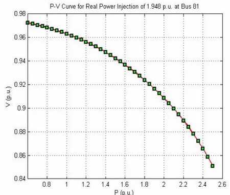
P-V Curve (81. Bus AMBARLI_A).……….………33

Figure 3.9

: P-V Curve (116. Bus ETILER)…..………...……33

Figure 3.10 :

Q-V Curve (5. Bus IEEE20)………..………35

Figure 3.11 :

Q-V Curve (9. Bus IEEE20)………...…..…………...…...35

Figure 3.12 : Q-V Curve (19. Bus IEEE20)…………..………...…....36

Figure 3.13 : Q-V Curve (24. Bus 1IEDIRNE_A) ………...36

Figure 3.14 : Q-V Curve (81. Bus AMBARLI_A)……….37

(13)

LIST OF ABBREVIATIONS

Active

Power-Voltage : P-V

Institute of Electrical and Electronics Engineer

:

IEEE

Kirchhoff’s

Current

Law

: KCL

per unit

: p.u.

Reactive Power-Voltage

: Q-V

Türkiye Elektrik İşletmeleri Anonim Şirketi

: TEİAŞ

(14)

LIST OF SYMBOLS

Admittance

:

Y

Current

: I

Jacobian matrix

:

J

Reactive power

: Q

Real power

: P

Transformation

ratio

:

1:a

Voltage

magnitude

:

V

(15)

1. INTRODUCTION

1.1 BACKGROUND

Today’s power transmission systems become heavily loaded and more stressed due to

increased loads and large inter-utility power transfers. Under these circumstances, a

number of voltage security problems have arisen within electric power systems

[Taylor 1994], [Abed et. al. 1998]. Efficient system operation is becoming

increasingly threatened because of problems of voltage instability and collapse

[Overby et. al. 1994], [Bilir 2000]. The term voltage instability is used to describe

situations in which a disturbance, an increase in load, or other system change causes

bus voltages to vary significantly from their desired operating range in such a way

that standard mechanisms of operator intervention or automatic system controls fail to

stop this deviation. If bus voltages ultimately fall in a more rapid decline, leading to

loss of portions of the network, the term voltage collapse is used. The voltage related

threats to system security are expected to become more severe as demand for electric

power rises, while economic and environmental concerns limit the construction of

new transmission and generation facilities.

Voltage security means the ability of a system, not only to operate stably, but also to

remain stable following contingencies or load increases [IEEE Spec. Pub. 1990]. It

often means the existence of considerable margin from an operating point to the

voltage instability point following contingencies. The margin could be the real power

transfer on a specific line, loading within an area, or reactive power margin at some

buses in a studied area. Industry experience has shown that voltage stability analysis

is often suited to static analysis [Bose et. al. 2001], [IEEE Spec. Pub. 1990], [Abed et.

al. 1998].

A slow-spreading, uncontrollable decline in voltage, known as voltage collapse, is a

specific type of transmission system voltage instability. Voltage collapse results when

generators reach their field current limits which cause a disabling of their excitation

voltage control systems. Voltage collapse has recently caused major blackouts in a

number of different countries around the world [Dobson et. al. 2002].

(16)

In order to reduce the possibility of voltage collapse in a power system, system

planning is performed by many utility companies. First, a mathematical model of the

basic elements of the power system, and their interconnection, is constructed. These

basic elements include generating stations, transmission lines, and sources of reactive

reserves. Next, various computational techniques for analyzing system stability are

performed using a suitably programmed computer.

In mathematical terms, voltage collapse occurs when equilibrium equations

associated with the mathematical model of the transmission system do not have

unique local solutions. This results either when a local solution does not exist or when

multiple solutions exist. The point at which the equilibrium equations no longer have

a solution or a unique solution is often associated with some physical or control

capability limit of the power system. Such a point is the critical point; its detection

plays a major role in determining voltage security margins [Huang and Abur 2002].

Current methods for assessing proximity to classic voltage instability are based on

some measure of how close a power-flow Jacobian is to a singularity condition, since

a singular power-flow Jacobian implies that there is not a unique solution [Mohn and

Zambroni de Souza 2006]. Two of these proximity measures are:

1) The real power flow-voltage level (P-V) curve margin

2) The reactive power flow-voltage level (Q-V) curve margin

Power flow based methods, P-V curves and Q-V curves are widely used. These two

methods determine steady-state loadability limits which are related to voltage stability

[Taylor 1994].

1.2 LITERATURE REVIEW

The fundamentals of modeling power systems, specifically concentrating on voltage

and reactive power topics, are covered well in [Taylor 1994] and [Kundur 1994].

Issues on power system static security analysis are introduced in [Wood and

Wollenberg 1996]. This gives the background on the significant roles played by

security analysis in modern bulk power system operation and control. Voltage

(17)

The problems of voltage stability and collapse have attracted numerous research

efforts from power systems researchers [Dobson and Chiang 1989], [IEEE Spec. Pub.

1990], [Greene et. al. 1999], [Van Cutsem and Vournas 2008]. Many voltage stability

margins and indices have been proposed and used throughout the world for voltage

security analysis. One category of voltage stability indices is based on eigenvalue and

singular value analysis of the system Jacobian matrix [Gao et. al. 1992], [Lof et. al.

1993], [Canizares et. al. 1996]. The idea is to detect the collapse point by monitoring

the minimum eigenvalue or singular value of the system Jacobian, which becomes

zero at the collapse point. With the analysis of the associated eigenvectors or singular

vector, one can determine the critical buses in the system by the right vector, and the

most sensitive direction for changes of power injections by the left vector. However,

the behavior of these indices is highly nonlinear; that is, they are rather insensitive to

system parameter variations. In addition, for large systems, this process is also

computationally expensive.

The more prominently applied methods in voltage stability analysis are those that try

to define an index using the system load margin. The two most widely used are the

real power margin, P, associated with the P-V curve, and the reactive power margin,

Q, associated with the Q-V curve. The P margin can be calculated using the point of

collapse method [Canizares et. al. 1992] or the power-flow continuation method

[Ajjarapu and Christy 1992]. In [Parker 1996], it is formulated as an optimization

problem. For fast calculation of the P margin, curve fitting methods are proposed to

calculate the limit of the nose curve [Ejebe et. al. 1996], [Chiang et. al. 1997].

Similarly, in [Greene et al. 1999], a sensitivity based linear/quadratic estimation

method is proposed.

The P-V curve-based and Q-V curve-based margins are the two most widely-used

static methods for voltage security assessment [Bose et. al. 2001]. For voltage

security, Q-V curve interpretations of energy measures are provided by [Overby et.

al. 1994]. The V-Q curve power-flow method is discussed in [Chowdhury and Taylor

2000]. Using P-V and Q-V curves, Jaganathan and Saha [Jaganathan and Saha 2004]

conduct a voltage stability analysis to evaluate the impact of embedded generation on

distribution systems with respect to the critical voltage variations and collapse

(18)

constraint reactive implicit coupling method to trace P-V and Q-V curves. A

measurement-based Q-V curve method, which can measure on-line part of the Q-V

curve in the vicinity of the operating point employing some adjustable parameters and

special compensation method to implement the measurement procedure, is proposed

in [Huang et. al. 2007].

1.3 STATEMENT OF THE PROBLEM AND METHODOLOGIES

Voltage security assessment is of major concern in electric utility companies. With

technological change and utility deregulation, the electric industry moves toward an

open-access market. This transition is expected to place further stress on the

transmission network due to an increase in power transactions carried over the

transmission grid. Such heavily-loaded systems lead to reduced operating margins.

Under these circumstances, utilities and system operators need to know voltage

security margins for secure operations and power transactions.

Knowing that voltage security plays a crucial role in operations of power systems, we

conduct a research study to assess margins of voltage security of the two power

systems; one of which is the 20-bus IEEE system and the other is the 225-bus system

of Istanbul Region. For our research study, we need power-flow solutions of the

given systems. The power flow is widely used in power system analysis. The solution

of power flow predicts what the electrical state of the network will be when it is

subject to a specified loading condition. The result of the power flow is the voltage

magnitude and the angle at each bus of the system. Power-flow solutions are closely

associated with voltage stability analysis. It is an essential tool for voltage stability

evaluation. Much of the research on voltage stability deals with the power-flow

computation methods. Regarding security margin calculations, we develop a

power-flow program as the tool for our analysis. We write the codes for the program in

MATLAB environment.

Developing the power-flow program is one of the major parts our research study. Let

us describe the power-flow problem. Consider an electric power system with n buses

(19)

pv

n

buses at which active power P and voltage magnitude

V

are specified (these

are PV buses), and

n

_pq

buses at which active and reactive power (P, Q) are specified

(these are PQ buses). The single swing bus is a generation bus which is usually

centrally located in the system; the voltage magnitude and phase angle (δ ) are

specified at this bus. The PV buses are mostly generation buses at which the injected

active power is specified and held fixed by turbine settings. A voltage regulator holds

V

fixed at PV buses by automatically varying the generator field excitation. This

variation causes the generated reactive power to vary in a way as to bring the terminal

voltage magnitude to the specified value. The PQ buses are primarily load buses.

Evidently,

.

1 +

+

=

n

_pv

n

_pq

n

At PV buses,

quantity

specified

i

P

=

pv

n

i

quantity

specified

i

V

=

,

=

buses.

At PQ buses,

quantity

specified

i

P

=

pq

n

i

quantity

specified

i

Q

=

,

=

buses.

At the swing bus,

quantity

specified

i

V

=

specified

quantity

i

,

δ

swing bus.

We need to calculate i

δ

and i

Q at PV buses,

V

_i

and i

δ

at PQ buses, and i

P and

i

Q at the swing bus. In order to obtain these values via bus voltages and bus injection

currents, we solve the system of (

2 n

_pv

+

2 n

_pq

+

2 =

2 n

) power-flow equations

(

)

∑

=

−

=

n j ij j i ij j i i

V

Y

P

1

cos

δ

θ

(1.1)

(

)

∑

=

−

=

n j ij j i ij j i i

V

Y

Q

1

sin

δ

θ

(1.2)

(20)

using the node-voltage equation in the matrix form

I

=

YV

,

where I is the bus injection-current vector,

V

is the bus voltage vector, and Y is the

bus admittance matrix. As easily seen in equations (1.1) and (1.2), the power-flow

problem is a nonlinear problem because of the sinusoidal terms and the product of

voltage magnitudes. For such a system of equations, there are no closed-form

solutions. However, we obtain numerical solutions using Newton-Raphson method.

In our program, starting with initial guess with voltage magnitudes of 1.0 p.u and

voltage angles of 0 degrees, we calculate the power-flow solution under the contraints

of reactive power limits of generators with the tolerance of 0.01 p.u.. For the two

sample power systems, the 20-bus IEEE system and the 225-bus system of Istanbul

Region, we run our power-flow program and obtain the solutions successfully.

We assess the voltage security by computing security margins via P-V and Q-V

curves. Our major tool is the power-flow program to generate P-V and Q-V curves.

For the computation of security margins, we choose candidate buses from load buses

to apply incremental changes in real power and reactive power. At each candidate

bus, we start with the base case solution of the power flow. To draw the P-V curve for

a candidate bus, we increase real power by 0.2 p.u. at each time and run the

power-flow program successively until the power power-flow does not converge. In this way, we

have successive values of the real power P and the corresponding voltage magnitudes

at the candidate bus. Using these values, the P-V curve is drawn for the real power

and the voltage magnitude at the candidate bus. To fine tune the computation of the

margins, between the last step at which the power flow converges and the next step at

which it does not converge, we change the value of increment to 0.1 p.u. and 0.05 p.u.

It means that we approach the nose of the curve, where increase in real power results

in non-convergence of the power-flow convergence, by the tolerance of 0.05 p.u.. The

difference between the real power at the nose of the curve and that at the base case

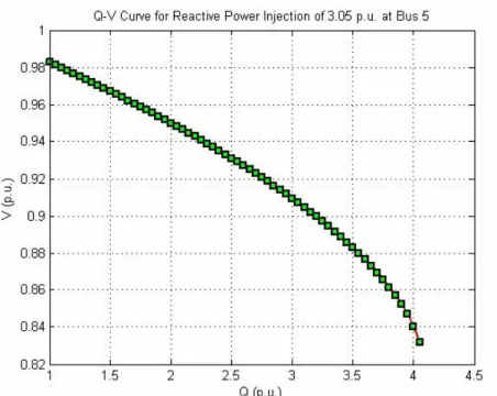
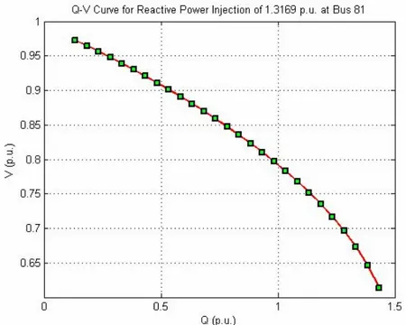
gives the P-margin of the system at the candidate bus. To draw the Q-V curve for a

candidate bus, we apply the similar procedures as we perform to draw P-V curves.

(21)

2. POWER-FLOW ANALYSIS

2.1 INTRODUCTION

Power-flow analysis is a quite important concept for energy system planning,

operating and controlling. In this part, we discuss steady-state analysis of an

interconnected power system during normal operation. The system is assumed to be

operating under balanced three-phase steady-state conditions and is represented by a

single-phase network. The network contains hundreds of buses and branches with

impedances specified in per unit on a common MVA base [Saadat 2004].

Network equations can be formulated in various forms. However, the node-voltage

method is commonly used, since it is the most suitable form for many power system

analyses. The formulation the network equations in the nodal admittance form results

in complex linear simultaneous algebraic equations in terms of node currents. When

node currents are specified the set of linear equations can be solved for the node

voltages. However, in a power system, powers are known rather than currents.

Therefore, the resulting equations in terms of power, known as the power-flow

equation, become nonlinear and must be solved by iterative techniques. Power-flow

studies are the backbone of power system analysis and design. They are necessary for

planning, operation, economic scheduling, and exchange of power between utilities.

2.2 BUS-ADMITTANCE MATRIX

In order to obtain the node-voltage equations, consider the simple power system in

shown in Figure 2.1 where impedances are expressed in per unit on a common MVA

base and for the sake of simplicity, resistances are neglected. Since the nodal solution

is based upon Kirchhoff’s current law (KCL), impedances are converted to

admittance [Saadat 2004]; that is,

ij ij ij ij

jx

r

z

y

+

=

1

1 (2.1)

(22)

Figure 2.1: The impedance diagram of a simple system

Figure 2.2: The admittance diagram of the system in Figure 2.1

The circuit has been redrawn in Figure 2.2 in terms of admittances and transformation

to current sources. Applying KCL to the independent nodes 1 through 4 results in

(

)

(

)

(

)

(

)

(

)

(

)

(

)

(

4 3

)

34 4 3 34 1 3 13 2 3 23 3 2 23 1 2 12 2 20 2 3 1 13 2 1 12 1 10 1

0

0 V

V

y

V

y

V

y

V

y

V

y

V

y

V

y

I

V

y

V

y

V

y

I

−

=

−

+

−

+

−

=

−

+

−

+

=

−

+

−

+

=

(2.2)

(23)

(

)

(

)

(

)

3 34 4 34 4 34 3 34 23 13 2 23 1 13 3 23 2 23 12 20 1 12 2 3 13 2 12 1 13 12 10 1

0

0 V

y

V

y

V

y

V

y

V

y

V

y

V

y

V

y

V

y

I

V

y

V

y

V

y

I

−

=

−

+

−

=

−

+

−

=

−

+

=

(2.3)

We introduce the following admittances

34 43 34 23 32 23 13 31 13 12 21 12 34 44 34 23 13 33 23 12 20 22 13 12 10 11

y

Y

y

Y

y

Y

y

Y

y

Y

y

Y

y

Y

y

Y

−

=

−

=

−

=

−

=

+

=

+

=

+

=

(2.4)

The node equation reduces to

4 44 3 43 2 42 1 41 4 4 34 3 33 2 32 1 31 3 24 3 23 2 22 1 21 2 4 14 3 13 2 12 1 11 1

V

Y

V

Y

V

Y

V

Y

I

V

Y

V

Y

V

Y

V

Y

I

V

Y

V

Y

V

Y

V

Y

I

V

Y

V

Y

V

Y

V

Y

I

+

=

+

=

+

=

+

=

(2.5)

In above network, there is no connection between bus 1 and 4. Thus,

Y

₁₄

= Y

₄₁

=

0 ;

similarly

Y

₂₄

= Y

₄₂

=

0 .

Extending the above relation to an n bus system, the node-voltage equation in matrix

form is

(24)

⎥

⎦

⎤

⎢

⎣

⎡

⎥

⎦

⎤

⎢

⎣

⎡

=

⎥

⎦

⎤

⎢

⎣

⎡

n i nn ni n n in ii i i n i n i n i

V

Y

I

#

"

#

"

#

"

#

2 1 2 1 2 1 2 2 22 21 1 1 12 11 2 1

(2.6)

or

I

bus

= Y

bus

V

bus

(2.7)

I

bus

is the vector of the injected bus currents. The current is positive when flowing

toward the bus and it is negative if flowing away from the bus. V

bus

is the vector of

bus voltages measured from the reference node. Y

bus

is known as the bus admittance

matrix. The diagonal element of each node is the sum of admittances connected to it.

It is known as the self-admittance

∑

=

n j ij ii

y

Y

0

j

≠ .

i

(2.8)

The off-diagonal element is equal to the negative of the admittance between the

nodes. It is known as the mutual-admittance

Y

ij

=

Y

ji

=

y

ij

. (2.9)

2.3 TAP CHANGING TRANSFORMERS

Transformers can be used to control the real and reactive power flows in a circuit. We

now develop the bus admittance equations to include such transformers in a power

flow studies. Figure 2.3 is detailed representation of the ideal transformer. The

(25)

Figure 2.3: Transformer with tap setting ratio a:1

Admittance

y in per unit is the corresponding of the per unit impedance of the

_t

transformer which has the transformation ratio 1:a as shown. In the case of phase

shifting transformers, a is a complex number. Consider a fictitious bus x between the

turn ratio and admittance of the transformer. Since the complex power on either side

of the ideal transformer is the same, it follows that if the voltage goes through a

positive phase angle shift, the current will go through a negative phase angle shift.

For the assumed direction of currents, we have [Saadat 2004], [Grainger 1994]

j x

V

a

V

=

1 (2.10)

j i

a

I

=

−

*

(2.11)

The current

I can be expressed by

i

)

(

V

_i

V

_x

t

y

i

I

=

−

(2.12)

Substituting for x

V , we have

V

_j

a

t

y

i

V

t

y

i

I

=

−

(2.13)

From 2.11, we have

i

I

a

j

I

*

1 −

=

(2.14)

Substituting for iI from 2.13, we have

V

_j

a

t

y

i

V

a

t

y

j

I

2 *

+

−

=

(2.15)

(26)

Writing (2.13) and (2.15) in the matrix form results in

⎥

⎦

⎤

⎢

⎣

⎡

⎥

⎦

⎤

⎢

⎣

⎡

−

=

⎥

⎦

⎤

⎢

⎣

⎡

j

V

i

V

a

t

y

a

t

y

a

t

y

t

y

j

I

i

I

2 *

(2.16)

2.4 NEWTON-RAPHSON METHOD

The most widely-used method for solving simultaneous algebraic equations is the

Newton-Raphson method. Newton-Raphson’s method is a successive approximation

procedure based on an initial estimate of the unknown and the use of Taylor’s series

expansion. Consider the solution of the one-dimension equation given by

f

( )

x

=

c

(2.17)

If

( )0

x

is an initial estimate of the solution, and

Δ

x

( )0

is a small deviation from the

correct solution, we must have

f

(

x

( )0

+

Δ

x

( )0

)

=

c

(2.18)

Expanding the left-hand side of the above equation in Taylor’s series about

( )0

x

yield

( )

( ) ( )

(

_x

( )

)

_c

dx

f

d

x

dx

df

x

f

_⎟⎟

Δ

+

=

⎠

⎞

⎜⎜

⎝

⎛

+

Δ

⎟

⎠

⎞

⎜

⎝

⎛

+

0 2

"

0 2 2 0 0 0

!

2

1 _(2.19)

Assuming the error

( )0

x

Δ

is very small, the higher-order terms can be neglected,

which results in

( ) ( )0 0 0

x

df

c

⎟

Δ

⎠

⎞

⎜

⎝

⎛

≅

Δ

,

(2.20)

(27)

where

( )0

( )

( )0

x

f

c

=

−

Δ

.

(2.21)

Adding

( )0

x

Δ

to the initial estimate will result in the second approximation

( ) ( ) ( ) 0 1 0 (0)

(

)

c

x

df

dx

Δ

=

+

.

(2.22)

Use of this procedure yields the Newton-Raphson algorithm

( )k

( )

( )k

c

f x

Δ

= −

(2.23)

(k ) ( )k ( )k

x

+1

=

+

Δ

(2.24)

( ) ( ) ( )

(

)

k k k

c

x

df

dx

Δ

=

.

(2.25)

The last equation can be rearranged as

( )k ( )k ( )k

x

J

c

=

Δ

,

(2.26)

where

( ) k k

dx

df

J

⎟

⎠

⎞

⎜

⎝

⎛

=

(2.27)

(28)

( )

( ) ( ) ( ) ( ) ( ) ( ) ( )

( )

( ) ( ) ( ) ( ) ( ) ( ) ( ) 2 0 0 2 0 2 0 2 2 0 1 0 1 2 0 2 1 0 0 1 0 2 0 2 1 0 1 0 1 1 0 1

c

x

f

x

f

x

f

c

x

f

x

f

x

f

n n n n

=

Δ

⎟⎟

⎠

⎞

⎜⎜

⎝

⎛

∂

+

Δ

⎟⎟

⎠

⎞

⎜⎜

⎝

⎛

∂

+

Δ

⎟⎟

⎠

⎞

⎜⎜

⎝

⎛

∂

+

=

Δ

⎟⎟

⎠

⎞

⎜⎜

⎝

⎛

∂

+

Δ

⎟⎟

⎠

⎞

⎜⎜

⎝

⎛

∂

+

Δ

⎟⎟

⎠

⎞

⎜⎜

⎝

⎛

∂

+

"

#

( )

( ) ( ) ( ) ( ) ( ) ( ) ( ) n n n n n n n

x

c

x

f

x

f

x

f

_⎟⎟

Δ

=

⎠

⎞

⎜⎜

⎝

⎛

∂

+

Δ

⎟⎟

⎠

⎞

⎜⎜

⎝

⎛

∂

+

Δ

⎟⎟

⎠

⎞

⎜⎜

⎝

⎛

∂

+

0 0 0 2 0 2 0 1 0 1 0

_"

or in the matrix form

( )

( ) ( ) ( ) ( ) ( ) ( ) ( ) ( ) ( ) ( ) ( ) ( )

⎥

⎦

⎤

⎢

⎣

⎡

Δ

⎥

⎦

⎤

⎢

⎣

⎡

⎟⎟

⎠

⎞

⎜⎜

⎝

⎛

∂

⎟⎟

⎠

⎞

⎜⎜

⎝

⎛

∂

⎟⎟

⎠

⎞

⎜⎜

⎝

⎛

∂

⎟⎟

⎠

⎞

⎜⎜

⎝

⎛

∂

⎟⎟

⎠

⎞

⎜⎜

⎝

⎛

∂

⎟⎟

⎠

⎞

⎜⎜

⎝

⎛

∂

⎟⎟

⎠

⎞

⎜⎜

⎝

⎛

∂

⎟⎟

⎠

⎞

⎜⎜

⎝

⎛

∂

⎟⎟

⎠

⎞

⎜⎜

⎝

⎛

∂

=

⎥

⎦

⎤

⎢

⎣

⎡

−

0 0 2 0 1 0 0 2 0 1 0 2 0 2 2 0 1 2 0 1 0 2 1 0 1 1 0 0 2 2 0 1 1 n n n n n n n n n

x

f

x

f

x

f

x

f

x

f

x

f

x

f

x

f

x

f

c

f

c

f

c

#

"

#

"

#

In short form, it can be written as

( )k ( )k ( )k

X

J

C

=

Δ

(2.28)

Consequently, the Newton-Raphson algorithm for n-dimensional case becomes

(k 1) ( )k ( )k

X

+

=

X

+ Δ

X

(2.29)

( )k

J

is called the Jacobian matrix. Newton’s method, as applied to a set of nonlinear

equations, reduces the problem to solving a set of linear equations in order to

determine the values that improve the accuracy of the estimes.

2.5 POWER-FLOW SOLUTION

(29)

single-phase model is used. Four quantities are associated with each bus. There are

voltage magnitude

V

, phase angle

δ , real power P , and reactive powerQ . The

system buses are generally classified into three types. They are:

Swing bus:

A bus, known as reference bus or slack bus, where the voltage magnitude

and phase angle are specified. At this bus, the active power and the reactive power are

unknown.

Load buses:

At these buses are called P-Q buses. The active and reactive powers are

specified; the voltage magnitude and voltage angle are unknown.

Generator buses:

At these buses are called P-V or regulated buses. The real power

and the voltage magnitude are specified; the voltage angle and the reactive power are

unknown.

The power-flow problem is solving the resulting nonlinear system of algebraic

equation suitable for the computer solution. In general, two methods are, used to

solve these nonlinear equations; they are Gauss-Seidel and Newton- Raphson.

However, in power industry, Newton-Raphson is preferred, because it is more

efficient for large networks, quadratic convergence and equations are cast in natural

power system form. In this respect, we have followed the preference in industry and

have used Newton - Raphson method in our program.

In this part, the bus-admittance matrix is formulated, the Newton-Raphson method is

explained, and it is employed in the solution of power-flow problems [Saadat 2004].

Consider a typical bus of a power system network as shown Figure 2.4 application of

the KCL to this bus results in

₍

(

₎

)

(

)

(

)

n in i i i in i i n i in i i i i i i i

V

y

V

y

V

y

V

y

V

y

V

y

V

y

V

y

I

−

+

=

−

+

−

+

−

+

=

"

2 2 1 1 1 0 2 2 1 1 0

or

∑

= =

−

=

i n ij n ij j i

V

y

V

I

0 1

j

≠

i

(2.30)

(30)

Figure 2.4: A typical bus of the power flow system

The real and reactive power at bus i is

* i i i i

jQ

V

I

P

+

=

(2.31)

or

_* i i i i

V

jQ

P

I

=

−

(2.32)

Substituting for

I in (2.30)

i

∑

= =

−

=

−

n j j ij n j ij i i i i

V

y

V

jQ

P

1 0 *

j

≠ (2.33)

i

The above equation is the mathematical formulation of the power-flow problem

results. This equation is a nonlinear equation, so it must be solved by iteration

techniques.

(31)

2.6 POWER-FLOW SOLUTION BY NEWTON-RAPHSON

The Newton-Raphson method is found to be more efficient and practical for large

power systems. In this method, the number of iterations required to obtain a solution

is independent of the system size, but more functional evaluations are required at each

iteration. For the typical bus of the power system shown in Figure 4, the equation of

the current entering bus i can be rewritten in terms of the bus admittance matrix as

∑

=

n j j ij i

Y

V

I

1

(2.34)

In the above equation j includes bus i. Expressing this equation in polar form,

∑

=

+

∠

=

n j j ij j ij i

Y

V

I

1

δ

θ

(2.35)

The complex power at bus i is

P

i

jQ

i

V

i

I

i

*

=

−

(2.36)

Then substituting from (2.35) for

I in (2.36),

i

∑

=

+

∠

−

∠

=

−

n j j ij j ij i i i i

jQ

V

Y

V

P

1

δ

θ

δ

(2.37)

Separating the real and imaginary parts,

∑

(

)

=

−

=

n j ij j i ij j i i

V

Y

P

1

cos

δ

θ

(2.38)

∑

(

)

=

−

=

n j ij j i ij j i i

V

Y

Q

1

sin

δ

θ

(2.39)

The last equations constitute a set of nonlinear algebraic equations in terms of the

independent variables, voltage magnitude in per unit and phase angle in radians. If the

Newton-Rahpson method is applied these equations,

(32)

( ) ( ) ( ) ( ) 2 2 _| 2 2 2 2 | ( ) ( ) ( ) ( ) | 2 2 | ( ) ( ) ( ) ( ) 2 2 _| 2 2 2 2 |

( )

2 ( )

( )

2 ( )

k k k k P P P P V V n n k k k k P_n P_n P_n P_n V V n n k k k k Q Q Q Q V V n n Qn

k

P

k

Pn

k

Q

k

Qn

δ δ δ δ δ δ ∂ Δ∂ ∂ ∂ ∂ ∂ ∂ ∂ ∂ ∂ ∂ ∂ ∂ ∂ ∂ ∂ = −− −− −− −− −− −− ∂ ∂ ∂ ∂ ∂ ∂ ∂ ∂ ∂

Δ

− − −

Δ

⎡

⎤

⎢

⎥

⎢

⎥

⎢

⎥

⎢

⎥

⎢

⎥

⎢

⎥

⎢

⎥

⎢

⎥

⎢

⎥

⎣

⎦

" # # % # # % # " # " " # % # # % #

#

( ) ( ) ( ) ( ) | 2 2

( )

2 ( )

( )

2 ( )

k _Q k _Q k _Q k n n n V V n n

k

n

k

V

k

Vn

δ δ

δ

⎡ ⎤ ⎡ ⎤ ⎢ ⎥ ⎢ ⎥ ⎢ ⎥ ⎢ ⎥ ⎢ ⎥ ⎢ ⎥ ⎢ ⎥ ⎢ ⎥ ⎢ ⎥ ⎢ ⎥ ⎢ ⎥ ⎢ ⎥ ⎢ ⎥ ⎢ ⎥ ⎢ ⎥ ⎢ ⎥ ⎢ ⎥ ⎢ ⎥ ⎢ ⎥ ⎢ ⎥ ⎢ ⎥ ⎢ ⎥ ⎢ ⎥ ⎢ ⎥ ⎢ ⎥ ⎢ ⎥ ⎢ ⎥ ⎢ ⎥ ⎢ ⎥ ⎢ ⎥ ⎢ ⎥ ⎢ ⎥ ⎢ ⎥ ⎢ ⎥ ⎢ ⎥ ⎢ ⎥ ⎢ ⎥ ⎢ ⎥ ⎢ ⎥ ⎢ ⎥ ⎢ ⎥ ⎢ ⎥ ⎢ ⎥ ⎢ ⎥ ⎢ ⎥ ⎢ ⎥ ⎢ ⎥ ⎢ ⎥ ⎢ ⎥ ⎢ ⎥ ⎢ ⎥ ⎢ ⎥ ⎢ ⎥ ⎢ ⎥ ⎢ ⎥ ⎢ ⎥ ⎣ ⎦ ⎣ ⎦ ∂ ∂ ∂ ∂ ∂ ∂ ∂

Δ

Δ∂

−−−

Δ

" "

#

In short form, the above equation can be written as,

_⎥

⎦

⎤

⎢

⎣

⎡

Δ

⎥

⎦

⎤

⎢

⎣

⎡

=

⎥

⎦

⎤

⎢

⎣

⎡

Δ

V

J

Q

P

δ

4 3 2 1

(2.40)

The Jacobian matrix gives the linearized relationship between small changes in

voltage angle

k

i

δ

Δ

and the voltage magnitude

k i

V

Δ

with the small changes in real

and reactive power

k

i

P

Δ and

k i

Q

Δ

. Elements of the Jacobian matrix are partial

derivatives of the real and reactive power, evaluated at

k

i

δ

Δ

and

k i

V

Δ

.

For voltage- controlled buses, the voltage magnitudes are known. Therefore, if m

buses of the system are voltage-controlled, m equations involving Q

Δ and

Δ

V

and

the corresponding columns of the Jacobian matrix are eliminated. Accordingly, there

are

n

−

1 real power constraints and

n

−1

−

m

reactive power constraints, and the

Jacobian matrix is of order

(

2 n

−

1 −

m

) (

×

2 n

−

1 −

m

)

.

J

₁

is of the order

(

n

−

1 ) (

×

n

−

1 )

,

2

J

is of the order

(

n

−

1 ) (

×

n

−

1 −

m

)

,

J is of the order

₃

(

n

−

1 −

m

) (

×

n

−

1 )

, and

J

₄

is

(33)

J

₁

(

i

,

i

)

i

sin

(

)

i j ij i j ij j i i

P

V V Y

δ δ θ

δ

≠

∂

=

= −

−

∂

∑

(2.41)

J

₁

(

i

,

j

)

i

sin

(

)

i j ij i j ij j

P

V V Y

δ δ θ

δ

∂

=

−

∂

j

≠ (2.42)

i

The diagonal and off-diagonal elements of

J

₂

are

J

₂

(

i

,

i

)

i

2 cos( )

cos

(

)

i ii ii j ij i j ij j i i

P

V Y

V

θ

≠

δ δ θ

∂

=

+

−

∂

∑

(2.43)

J

₂

(

i

,

j

)

i

cos

(

)

i ij i j ij j

P

V Y

V

δ δ θ

∂

=

−

∂

j

≠ (2.44)

i

The diagonal and off-diagonal elements of

J are

₃

J

₃

(

i

,

i

)

i

cos

(

)

i j ij i j ij j i i

Q

V V Y

δ δ θ

δ

≠

∂

=

−

∂

∑

(2.45)

J

₃

(

i

,

j

)

i

cos

(

)

i j ij i j ij j

Q

V V Y

δ δ θ

δ

∂

=

= −

−

∂

j

≠ (2.46)

i

The diagonal and off-diagonal elements of

J

₄

are

J

₄

(

i

,

i

)

i

2 sin(

)

sin

(

)

i ii ii j ij i j ij j i i

Q

V Y

V

θ

≠

δ δ θ

∂

=

= −

−

+

−

∂

∑

(2.47)

J

₄

(

i

,

j

)

i

sin

(

)

i ij i j ij j

Q

V Y

V

δ δ θ

∂

=

−

∂

j

≠ (2.48)

i

The terms

( )k i

P

Δ

and

( )k i

Q

Δ

are the difference between the scheduled and calculated

values, known as the power residuals, given by

( ) ( ) ( )k i sch i k i

P

=

−

Δ

(2.49)

( ) ( ) ( )k i sch i k i

Q

=

−

Δ

(2.50)

(34)

The new estimates for bus voltages are

( ) ( ) ( )k i k i k i

δ

+1

=

+

Δ

_(2.51)

( ) ( ) ( )k i k i k i

V

+1

=

+

Δ

(2.52)

The procedure for power flow solution by the Newton-Raphson method is as follows:

1. Read system and load data.

2. Y

bus

is constitute.

3. Initialize δ ,

V

4. Calculate

Δ

P

and Q

Δ .

5. Calculate Jacobian matrix (2.41 through 2.48).

6. Solve for the voltage angle and magnitude (2.51 and 2.52).

7. Update the voltage magnitude and angles.

8. Check the stopping conditions. If met then terminate, else go to step 3.

( ) ( )

_ε

ε

≤

Δ

≤

Δ

k i k i

Q

P

(2.53)

2.7 LINE FLOW AND LOSSES

After the iterative solution of bus voltage, the next step is the computation of line

flows and line losses. Consider the line connecting the two buses i and j in Figure

2.5. The line current

I , measured at bus

_ij

i and defined positive in the direction

(35)

Figure 2.5: Transmission line model for calculating line flows

i

→

j is given by

I

_ij

= +

I

_l

I

_i₀

=

y V

_ij

(

_i

−

V

_j

)

+

y V

_i₀ _i

(2.54)

The line current

I measured at bus j and defined positive in the direction j

ji

→

i is

given by

I

ji

= − +

I

l

I

j0

=

y V

ij

(

j

−

V

i

)

+

y V

j0 j

(2.55)

The comlex powers

S from bus i and j and

ij

S from bus j to i are

ji

* ij i ij

S

=

V I

(2.56)

* ji j ji

S

=

V I

(2.57)

The power loss in line i

→

j is the algebraic sum of the power flows determined from

(2.56 and 2.57)

SL

_ij

=

S

_ij

+

S

_ji

(2.58)

2.8 POWER-FLOW PROGRAM

The power-flow computer program (called load flow) is the basic tool for invetigating

these requirements. This program computes the voltage magnitude and voltage angle

at each bus in a power system. Real power and reactive power flows for all equipment

interconnecting the buses, as well as equipment losses, are also computed. Both

existing power system and proposed changes including new generation and