Lecture 2 Laplace rev

(1)

1

EE 4314 - Control Systems

LECTURE 2

REVIEW OF LAPLACE TRANSFORM

LAPLACE TRANSFORM

The Laplace transform is very useful in analysis and design for systems that are linear and time-invariant (LTI). Beginning in about 1910, transform techniques were applied to signal processing at Bell Labs for signal filtering and telephone long-lines communication by H. Bode and others. Transform theory subsequently provided the backbone of Classical Control Theory as practiced during the World Wars and up to about 1960, when State Variable techniques began to be used for controls design. Pierre Simon Laplace was a French mathematician who lived 1749-1827, during the age of enlightenment characterized by the French Revolution, Rousseau, Voltaire, and Napoleon Bonaparte.

Given a time function f(t), its unilateral Laplace transform is given by

∫

∞ − − = 0 ) ( ) (s f t e dt F st ,

where s=σ j+ ω is a complex variable. Different authors may take the lower limit as

+

0 (i.e. not including effects occurring exactly at time t=0) instead of 0 . The bilateral− Laplace transform has a lower limit of −∞ and is not as useful for feedback control theory as the ULT.

One may write

∫

∞ − − − = 0 ) ( ) (s f t e e dt F σt jωt

and, comparing this to the Fourier transform, one sees that f(t) may have a Laplace transform though its Fourier transform does not exist. This is due to the fact that the weighted function f(t)e−σt decays faster than f(t) so that its Fourier transform may exist.

The inverse Laplace transform is a complex integral given by

∫

+ − = σ ω ω σ π j j st ds e s F j t f ( ) 2 1 ) ( ,

(2)

where the integration is performed along a contour in the complex plane. Since this is tedious to deal with, one usually uses the Cauchy theorem to evaluate the inverse transform using st e s F of residues enclosed t f( )=Σ ( ) .

In this course we shall use lookup tables to evaluate the inverse Laplace transform. In this course we shall use following notation for the unit test signals:

Note that each function is the integral of the previous function.

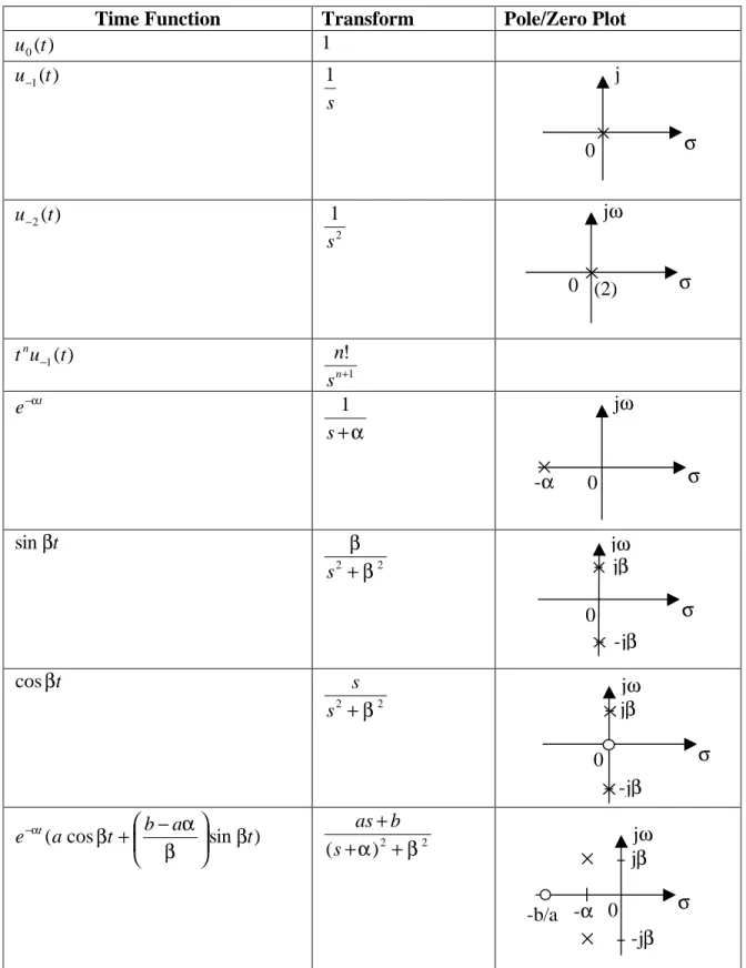
An abbreviated table of Laplace transforms is given here. The text has a more detailed table. Note that we are dealing with the 1-sided transform so that all time functions should be considered to be multiplied by the unit step.

It is important to represent a complex pair of poles in a good way. We shall not split a complex pole pair into two single roots using 'j'. Instead, we shall write

2 2

)

(s+α +β . Note that this has roots where:

β α β α β α β α j s j s s s ± − = ± = + − = + = + + 2 2 2 2 ) ( 0 ) ( .

We shall discuss the complex pole pair in depth when we discuss system performance and second-order systems.

0 t u0(t) Unit impulse 0 t u-1(t) Unit step 1 0 t u-2(t) Unit ramp

(3)

3

Table of Laplace Transforms

Time Function Transform Pole/Zero Plot ) ( 0 t u 1 ) ( 1 t u₋ s 1 ) ( 2 t u₋ 2 1 s ) ( 1 t u tn − 1 ! + n s n t e−α α + s 1 t β sin 2 2 β β + s t β cos 2 2 +β s s ) sin cos (a t b a t e t β β α β α     − + − 2 2 ) ( +α +β + s b as σ j 0 σ jω 0 (2) σ jω 0 -α σ jω 0 jβ -jβ σ jω 0 jβ -jβ σ jω 0 -α jβ -jβ -b/a

(4)

PROPERTIES OF THE LAPLACE TRANSFORM

Several properties of the Laplace transform are important for system theory. Thus, suppose the transforms of x(t),y(t) are respectively X(s),Y(s). Then one has the following properties.

Laplace Transform Properties

Time-Domain Operation Frequency Domain Operation Linearity property ) ( ) (t by t ax + ) ( ) (s bY s aX +

Time scaling property ) (at x __a_ s X a 1 Time shifting property

) (t t0 x − 0 ) (s e st X −

Frequency shifting property

at e t x( ) − ) (s a X + Convolution property ) ( * ) (t y t x ) ( ) (s Y s X Differentiation Property ) ( ' t x ) 0 ( ) (s −x − sX Differentiation Property ) ( ) ( t xn ) 0 ( ) 0 ( ) ( − n−1 − − − (n−1) − n x x s s X s L Integration property

∫

∞ − t d x(τ ) τ −

∫

∞ + 0 ) ( 1 ) ( τ τ d x s s s X

In this table, a superscript enclosed in parenthesis denotes differentiation of that order. An asterisk denotes convolution,

∫

− = − = t t d t y x d y t x t y t x 0 0 ) ( ) ( ) ( ) ( ) ( * ) ( τ τ τ τ τ τ .

The upper and lower convolution limits are as shown since all of our time functions are causal (i.e. multiplied by the unit step) in this course.

Note that, in the integration property there is a correction term in the transform if the time function x(t) is not zero to the left of time t=0. Since all our functions are causal, this term is usually equal to zero in this course.

(5)

5

Erwin Schrodinger developed an elegant theory of quantum mechanics using the premise that position and momentum are Laplace transform pairs. This allowed him to show the importance of his famous wave equation. In this context, the time scaling property is known as the Heisenberg Uncertainty Principle. In fact, it states that if position is known more accurately (i.e. its probability density function is on a compressed scale), then momentum is known less accurately (i.e. its PDF is on an expanded scale). As an interesting final comment, it turns out that in quantum mechanics there are other transform pairs besides position/momentum. One of these is time/energy.

INITIAL AND FINAL VALUE THEOREMS

Two theorems are indispensable in feedback control design.

Initial Value Theorem (IVT).

) 0 ( ) ( lim ₋ = ∞ → sX s x s .

The IVT says that the (fast) transient behavior of x(t) is determined by the high-frequency content of its spectrum X(s).

Final Value Theorem (FVT).

) ( lim ) ( 0 lim t x s s sX s→ = →∞ .

The FVT says that the steady-state, or DC behavior, of x(t) is determined by the low-frequency content of its spectrum X(s).

Example

Let a time function x(t) have the transform

s s s s s X 3 4 3 ) ( ₃ ₂ 2 + + + −

= . Using the IVT and the FVT one can determine the initial and final values of x(t) without ever having to

find the function x(t) itself. This is very important for quick design insight later in the

course.

Both the IVT and the FVT rely on the quantity

s s s s s s sX 3 4 3 ) ( ₃ ₂ 3 + + + − = .

(6)

According to the IVT, taking the limit of sX(s) as s goes to infinity yields the initial value of x(0−)=−1. To take this limit note that the highest-order terms in the numerator and denominator dominate.

According to the FVT, taking the limit of sX(s) as s goes to zero yields the final value for x(t) of 1. To take this limit note that the lowest-order terms in the numerator and denominator dominate.

Taking the inverse transform (which we shall cover soon) of X(s) yields ) ( ) 1 ( ) (t e e 3 u ₁ t

x = − −t− −t ₋ . A sketch of this function is given below.

-1 1 x(t)

t 0