YAŞAR UNIVERSITY
GRADUATE SCHOOL OF NATURAL AND APPLIED SCIENCES
INVENTORY MANAGEMENT SYSTEM IN FOOD
INDUSTRY
Efe AKINCI
Thesis Advisor: Asst. Prof. Dr. Önder Bulut
Department of Industrial Management and Information Systems
Bornova – İZMİR
TEXT OF OATH
I declare and honestly confirm that my study titled “INVENTORY MANAGEMENT SYSTEM IN FOOD INDUSTRY” and presented as Master’s Thesis has been written without applying to any assistance inconsistent with scientific ethics and traditions and all sources I have benefit from are listed in bibliography and I have benefited from these sources by means of making references.
Contents
1. INTRODUCTION ... 1
1.1. BACKGROUND ... 1
1.2. SUPPLY CHAIN IN THE ORGANIZATION ... 2
1.3. PROBLEM STATEMENT ... 3
1.4. INVENTORY MANAGEMENT PROBLEMS (DEFECTS, İNVENTORY LEVELS, ALLOCATİON) ... 3
1.5. OBJECTİVES ... 4
2. LITERATURE REVIEW ... 5
2.1. INVENTORY MANAGEMENT ... 5
2.2. TYPE OF INVENTORY ... 6
2.3. ECONOMİC ORDER QUANTİTY (EOQ) ... 7
2.3.1. EOQ with Quantity Discounts ... 9
2.4. KANBAN/JUST-İN-TİME (JIT)SYSTEM ... 12
2.4.1. Definition of JIT ... 12
2.4.2. Toyota Pioneers Kanban and JIT ... 13
2.4.3. Benefits of JIT ... 13
2.4.4. Problems Associated with JIT ... 14
2.4.5. Implication of JIT ... 16
2.5. SUPPLY CHAİN MANAGEMENT (SCM) ... 16
2.6. LOGİSTİCS MANAGEMENT ... 19
2.6.1. Push System ... 20
2.6.2. Pull System ... 20
2.7. INVENTORY CONTROL ... 21
2.8. ABC ANALYSİS (INVENTORY) ... 23
2.8.1. Prioritization of the management attention... 23
2.8.2. Inventory management policies ... 25
2.8.3. Procurement and Warehouse Applications ... 26
2.8.4. Definition of 'Inventory Turnover' ... 27
2.8.5. Other Inventory Classification Techniques ... 27
3. AN INVENTORY MANAGEMENT STUDY FOR A FOOD COMPANY ... 29
3.1. ABOUT FOOD COMPANY ... 29
3.2. DATA ANALYSES ... 31
3.2.1. ABC Analyses ... 31
3.2.2. Results of ABC Analyses ... 40
3.3. TESTS FOR THE STOCK MANAGEMENT PRACTİCE ... 41
3.3.1. Optimization for Stock Holding ... 41
3.3.2. Comparison of Demands and Stocks ... 42
3.3.3. Comparison of Demands and Analyze Metods ... 46
3.3.4. Comparisons of the Methods for the Products ... 53
List of Figures
Figure 1 Supply Chain Cycle in the Food Company (Source:
Theprocessgroup.com White papers Logistics vs. Supply Chain ) ... 2
Figure 2 Level Of Risk ... 24
Figure 3 ABC Analyses in e-Commerce ... 25
Figure 4 Example for the data of Pareto Analyses ... 32
Figure 5 Example for the data of Pareto Analyses ... 33
Figure 6 Sales Quantity Change of A Products between January 2010 and October 2012 ... 35
Figure 7 Stocks Quantity Change of A Products between January 2010 and October 2012 ... 35
Figure 8 Sales Quantity Change of B Products between January 2010 and October 2012 ... 36
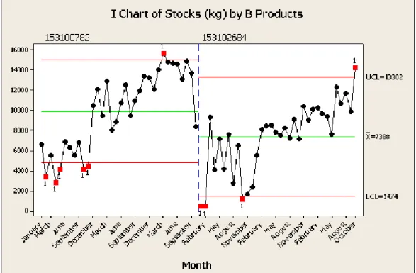
Figure 9 Stocks Quantity Change of B Products between January 2010 and October 2012 ... 37
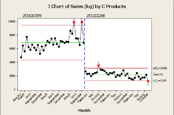
Figure 10 Sales Quantity Change of C Products between January 2010 and October 2012 ... 38
Figure 11 Stocks Quantity Change of C Products between January 2010 and October 2012 ... 38
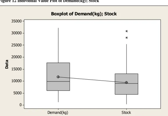
Figure 12 Individual Value Plot of Demand(kg); Stock ... 43
Figure 13 Box Plot of Demand and Stock ... 43
Figure 14 Histogram of Demand and Stock ... 44
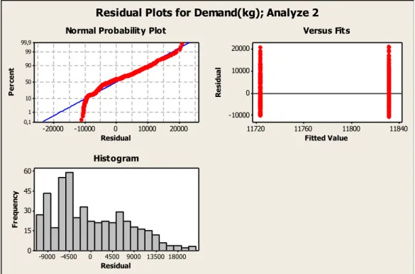
Figure 15 Residual Plot for Demand and Stock ... 44
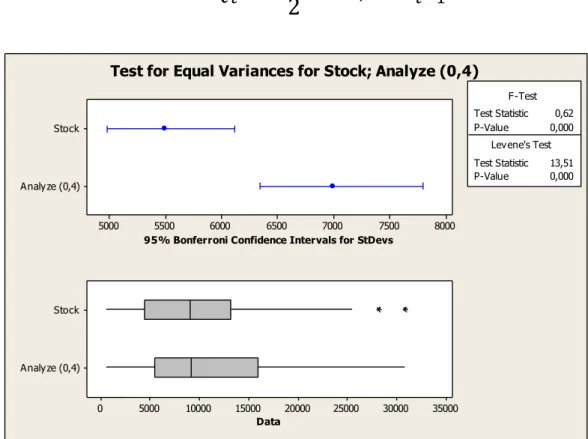
Figure 16 Test for Equal Variances for Stock; Analyze (0,4) ... 46
Figure 17 Test for Equal Variances for Stock; Analyze (0,5) ... 47
Figure 18 Individual Value Plot of Demand And Analyze (0,5) ... 48
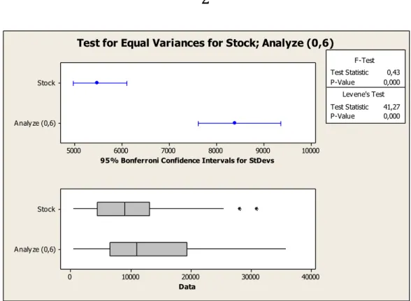
Figure 20 Boxplot od Demand and Analyze (0,5) ... 49 Figure 21 Residual Plots for Demand and Analyze (0,5) ... 49 Figure 22 Test for Equal Variances for Stock and Analyze (0,6) ... 51 Figure 23 Comparison of the Methods’ VariancesError! Bookmark not defined.
Figure 24 Test for Equal Variances for Demand and Analyze for the production 153100100 ... 53 Figure 25 Individual Value Plot for Demand and Analyze for the production 153100100 ... 54 Figure 26 Boxplot of Demand and Analyze for the production 153100100 .... 55 Figure 27 Test for Equal Variances for Demand and Analayze for the production 153100101 ... 55 Figure 28 Individual Value Plot of Demand and Analyze for the product 153100101 ... 57 Figure 29 Box Plot of Demand and Analyze for the product 153100101 ... 57 Figure 30 Test for Equal Variance between Demand and analyze for the product 153100102 ... 58 Figure 31 Indıvıdual Value Plot of Demand and Analyze for the product 153100102 ... 59 Figure 32 Box Plot of Demand and Analyze for the production 153100102 ... 60 Figure 33 Test for Equal Variances between Demand and analyze for the product 153102684 ... 61 Figure 34 Indıvıdual Value Plot of Demand and Analyze for the product 153102684 ... 62 Figure 35 Boxplot of Demand and Analyze for the product 153102684 ... 62 Figure 36 Test for Equal Variances for Demand and Analyze for the product 153100782 ... 63 Figure 37 Indıvıdual Value Plot of Demand and Analyze for the product 153100782 ... 64
Figure 38 Test for Equal Variances for Demand and Analyze for the Product 153100099 ... 65 Figure 39 Indıvıdual Value Plot of Demand and Analyze for the Product 153100099 ... 66 Figure 40 Boxplot of Deamand and Analyze for the product 153100099 ... 67 Figure 41 Test for Equal Variances for Demand and Analyze for the product 153102266 ... 67 Figure 42 Indıvıdual Value Plot of Demand and Analyze for the product 153102266 ... 69 Figure 43 Boxplot of Deamnd and Analyze for the product 153102266 ... 69
ABSTRACT
The optimum use of resources have become more important by the change of customer preferences and expectations in food industry. To perform accurate and consistent resource planning, changes in demand should be forecasted accurately and the inventroy management should be modeled according to these estimates.
With this study, the food company’ s sales, inventory and management plan for the new measurement estimates prepared by the method of statistical analysis. First of all segments of the material studied past plans and inventories. Statistical analysis of the new method was developed to improve the adequacy of the management process was measured. Depending on the administrative end of the study analysis are presented.
By the development of the new inventory forecasting methods the food company have been started to use it for the products that were used for the analyses. And also they are planning to implement the new methods for the other products.
ÖZET
Gıda Sanayinde müşteri tercih ve beklentilerinin değişimiyle birlikte taleplerdeki dalgalanmalar şirket kaynaklarının optimum kullanımı açısından önemli hale gelmiştir. Kaynak planlamalarının doğru ve tutarlı yapılabilmesi için taleplerdeki değişimler doğru tahminlenmeli ve stok yönetimi bu tahminler doğrultusunda yapılmalıdır.
Bu çalışmayla birlikte gıda firmasının satış, stok ve plan tahminlerinin yönetimine ilişkin yeni bir ölçümleme metodu ile istatistiksel analizi hazırlanmıştır. Öncelikle malzeme grupları bazında geçmiş planlar ve stoklar incelenmiştir. Yönetim sürecini iyileştirmek adına geliştirilen yeni yöntemin yeterliliği istatistiksel analizlerle ölçülmüştür. Çalışma sonunda analizlere bağlı olarak yönetsel öneriler sunulmuştur.
Firmanın ürün yönetim yöntemlerine uygun olarak geliştirilen yeni yöntem kullanılmaya başlanmıştır. Çalışmada yer alan firma diğer ürün grupları için de yeni yöntemi uygulamaya almayı planlamaktadır.
1. INTRODUCTION
The first chapter gives an introduction of the background of this study. Furthermore it gives an explanation of company’s problems. Then the research questions and purpose of this thesis are presented. The chapter ends with the delimitation of this study and the outline of following chapters.
1.1. Background
The American Production and Inventory Control Society (APICS) define inventory management as the branch of business management concerned with planning and controlling inventories (Toomey, 2000). Inventory management is a critical management issue for most companies – large companies, medium-sized companies, and small companies.
Logistics is all about managing inventory, whether the inventory is moving or staying, whether it is in a raw state, in manufacturing, or finished goods (Goldsby & Martichenko, 2005). Logistics and inventory management are embedded in each other and tied up closely. The “Bill of ‘Rights’” that logistics professionals often repeat is to deliver the right product to the right place, at the right time, in the right quantity and condition, and at the right cost (Goldsby et al., 2005). To make it happen, effective inventory management is a cornerstone.
Supply chain management coordinates and integrates all of these activities into a seamless process. During the process, inventory holding and warehousing play an important role in modern supply chains. A survey of logistics costs in Europe identified the cost of inventory as being 13 percent of total logistics costs, whilst warehousing accounted for a further 24 percent (European Logistics Association/AT Kearney, 2004). As well as being significant in cost terms, they are important in terms of customer service, with product availability being a key service metric and warehousing being critical to the success or failure of many supply chains (Frazelle, 2002).
Many large companies have saved millions of dollars in costs and decreased inventories while improving efficiency and customer satisfaction through various SCM techniques (Chapman et al., 2000).
1.2. Supply Chaın ın the Organızatıon
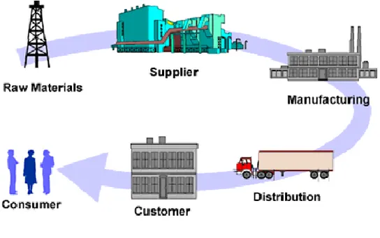
The supply chain is the series of links and shared processes that exist between Suppliers and Customers. These links and processes involve all activities from the acquisition of raw materials to the delivery of finished goods to the end consumer. Raw materials enter into a manufacturing organization via a supply system and are transformed into finished goods. The finished goods are then supplied to consumers through a distribution system. Generally, several companies are linked together in this process, each adding value to the product as it moves through the supply chain.
Figure 1 Supply Chain Cycle in the Food Company (Source: Theprocessgroup.com White papers Logistics vs. Supply Chain )
1.3. Problem Statement
The most common problem in inventory management is to attain optimal inventory levels. Decisions about how many of which products are to be stored in the warehouse, when to place the next order, the quantities to be ordered are some of the problems encountered every day. High level of inventory locks up the capital of any company. Customers on the other hand, lose confidence in the company and look elsewhere if there is no availability. This can reduce the profitability of the company and eventually crumple the company.
The science of balancing the right levels of inventory can be solved by modeling the inventory system into a mathematical model. This model can then be simulated and the result analyzed to reach the best practices in inventory management.
Goods in transit, obsolete stock, dead stock, fast and slow moving stock, back orders are all problems associated with managing inventory systems.
1.4. Inventory management problems (Defects, inventory levels, allocation)
Defects in the inventory and incoherent levels of inventory form a common problem in the area of inventory management planning. They affect the optimal operation of the inventory system. These problems are very common occurrence in most inventory systems. In different studies, they have been addressed using analytical models, queuing theory and deterministic programming techniques like integer programming. In order to properly understand the complexity of these problems, simulation models will be used to demonstrate the inventory system. To optimize stock allocation level and resources, a detailed analysis will be in Chapter 3. Another classic problem is the lead time. The objective is to minimize the average lead time and cost of holding high levels of inventory subject to the constraints on the throughput and the budget available.
1.5. Objectives
The purpose of this project is to investigate how a model for controlling a multi level inventory system can be used to calculate reorder points for Food Firm’s distribution centers. Furthermore, the project will, by simulation in the discrete event simulation software Extend, analyze how much the inventories could be reduced if a coordinated inventory control method is implemented, instead of the uncoordinated control system used today.
The analysis will be conducted using a sample of articles and the corresponding real case data from a geographically limited area. In this study, the goods flow chosen is the simplest possible multi level case: one distribution center and a number of retail stores. All articles included are replenished from that single distribution center. The chosen articles are taken from different price, frequency and service level categories. This means that even though only a fraction of the total number of articles is included, the results of the project should be representative for a larger number of other articles.
In addition to investigating how well a multi level inventory system will work, this project will also evaluate how well the service level measurement performed by the Food Firm today coincides with a theoretical definition of the service level called fill rate. This is defined as the proportion of total demand immediately satisfied from stock on hand.
2. LITERATURE REVIEW
This chapter reviews some of the research work that has been conducted so far in the field of Inventory Management, Economic Order Quantity (EOQ), Just In Time (JIT), Logistics Management, Supply Chain Management and Simulation Optimization.
2.1. Inventory Management
Inventory management deals with decisions regarding supply levels: the correct amount of material and the correct time to reorder. There are many reasons for a company to hold excess inventory; variation in demand and production; poor quality and unreliable suppliers and shippers. However, there are also good reasons to cut down the amount held in inventory: carrying cost, storage space and material handling. Thus an exchange has to be considered between the two situations.
Manufacturers are moving towards lean manufacturing and JIT, so companies are decreasing the amount of inventory being held. Retail stores are also applying the philosophy of JIT to reduce inventories and in turn reduce the associated costs at the store. But determining the exact amount that is needed to cover contingencies changes based on the situation faced by the company. There is one model that is commonly used to determine optimal order size. This is the Economic Order Quantity (EOQ) model. Another model that is also used is one that includes purchasing cost per unit in the total cost equation and aims at offering quantity discounts to customers that order large quantities. This is called the EOQ with Quantity Discounts.
Inventory management is defined as the direction and control of activities with the purpose of getting the right inventory in the right place at the right time in the right quantity in the right form and at the right cost. (Cudjoe, 2010)
Inventory is an important current asset with far reaching financial ramifications which deserves very organizations serious attention to ensure cost savings and optimum utilization of scare resources.
Cudjoe, (2010) explained that the terminology-Inventory was of American origin which was synonymous with stock associated with British authors. Assets in the form of goods, property or services held for sale in the ordinary course of business, in the process of production for sale or to be consumed in the production of goods for sale or in the rendering of services. In order words, inventory may exist in three main forms namely; Finished goods, Work in progress and raw materials.
Cudjoe, (2010) also said that Inventory was held for the following purposes;
i. To enable the organization to achieve economies of scale ii. To balance supply and demand
iii. To enable speculation activities
iv. To provide protection from uncertainties in demand and order cycle v. To act as a buffer between critical and interfaces within the channel of distribution.
2.2. Type of Inventory
Inventory can be classified based on the reasons for which they are accumulated. The categories of inventories include cycle stock, in-transit inventories, safety or buffer stock, speculative stock, seasonal stock and dead stock (Alema, 2011).
Cycle Stock is inventory that results from replenishment of inventory sold or used in production. It is required in order to meet demand under condition of certainty, that is, when the organization can predict demand and replenishment times (lead times) (Alema, 2011).
In-Transit inventories are items that are on the way from one location to another. They may be considered part of cycle stock even though they are not
available for sale or shipment until after they arrive at the destination. Safety or Buffer Stock is held in excess of cycle stock because of uncertainty in demand or lead time. Average inventory at a stock keeping location that experiences demand or lead time variability is equal to half the order quantity plus the safety stock (Alema, 2011).
Dead Stock refers to items for which no demand has been registered for some specified time.
2.3. Economic Order Quantity (EOQ)
Muckstadt et al., (2010) discussed that EOQ model was determined by minimizing the total annual cost incurred by the company by virtue of its ordering cost and carrying cost. The expression for total annual cost is:
𝑇𝐶 =𝑄 2. ℎ +
𝐷 𝑄. 𝑠
TC = Total annual cost, Q = Order Quantity D = Annual Demand S = ordering cost
H = Annual carrying cost per unit
They said that this model was based on the basic assumption that there was a single item, with deterministic demand and lead time, no shortages, and inventory was replenished in batches rather than continuously over a period of time.
Muckstadt et al., (2010) also said that the first component of this equation represented the inventory management costs and the second component represents the ordering cost.
Differentiating with respect to order quantity, the expression for EOQ was obtained as indicated in the equation below.
𝑄 = √2𝐷𝑠 ℎ
Q= Economic Order Quantity
The literature in the area of inventory management included different types of inventory models dealing with different real-world constraints. Many of these models are variations of the basic EOQ model where the alterations include the conditions that are encountered in the situation being studied. Despite these new conditions these models still try to determine the optimal order quantity, which is one area where the model developed in this research is different from other models for the EOQ.
Liberatore,(1979) discussed an EOQ model, with a few alterations to the assumptions on the basis of which the traditional EOQ model had been developed. Typically, demand always followed a pattern that could be traced by a probability distribution for analysis. The basic EOQ model, however, assumed that this demand was deterministic to simplify the calculations involved.
The traditional EOQ model also assumed that if the inventory is zero when the order was received then that particular order was lost. This was not the scenario in real life as orders may be backordered and fulfilled when the inventory was available. Liberatore, (1979) considered a more realistic situation for his model and developed an equation for the order size based on stochastic lead times and backlogged demand. The traditional equations of inventory theory with deterministic lead times and no backlogging were special cases of this model.
Kim et al., (2003) analyzed the suitability of using the Order Quantity Reorder point (Q, R) model where Q is the order quantity and R is the reorder point, for different situations in production/inventory systems. Kim et al., (2003) presented a Production/Inventory (Q, R) model that included the production lead times and the order replenishment lead times explicitly with the inventory costs. Comparisons between this model and the traditional (Q, R) model showed that the optimal order quantity and reorder point were different for each of the
models. This indicated that the average inventory and backorders would also be different and in turn, the estimated costs would also be different.
Therefore the value of lead time used in the models made a substantial difference in the costs. If the lead times were fixed then the costs in both the models would be the same. But in an actual manufacturing environment, the lead times were rarely constant and therefore the traditional model could severely overestimate or underestimate the order quantity and the reorder point. The authors also portrayed the impact of setup times on the quantity and they showed that the system stability depended on the order sizes. Kim et al., (2003) concluded by presenting the extensions that could be done to make this research more broad.
2.3.1. EOQ with Quantity Discounts
Quantity discounts are price reductions that are offered to the retailer when they place an order that is beyond a certain specific level. It is an incentive to the retailer to buy larger quantities. When quantity discounts are offered the retailer is forces to consider the possible benefit of ordering larger number of items with a lower price per item over the increase in the inventory costs that would be incurred by the retailer (Kim et al. 2003). The total quantity discount model can be written below:
𝑇𝐶 =𝑄 2. 𝐻𝐶 + 𝐷 𝑄. 𝑆 + 𝑃𝐷 Where, P = Unit Price
Including the purchasing cost in the total cost equation does not change the EOQ point but changes the total cost for the retailer since the unit costs for certain ranges are different. There are two cases of this model:
i. Carrying costs are constant: When carrying costs are constant, the EOQ remains, the same for all the curves.
ii. Carrying costs are a percentage of the purchasing cost: When the carrying costs are a percentage of purchasing cost per unit, the EOQ starting with the lowest price range is found. If this EOQ is feasible (i.e. falls in the correct quantity cost range), it is the EOQ for that model. If the EOQ found is infeasible, then the EOQ for the other prices are calculated starting form the next highest one. This procedure is continued until a feasible solution is reached.
There is a large body of research that has dealt with quantity discounts in the case of single supplier-single buyer situations and single supplier-multiple buyer situations. Stevenson (1993) had compiled a paper that reviewed the literature in determining lot sizes using the principle of quantity discounts. Stevenson (1993) categorized the literature based on whether the quantity discounts were all-units or incremental and also categorize from buyer’s or the seller’s perspective.
This section of the literature focuses on some of the research that has been done regarding the quantity discount model and modifications of the EOQ model is this regard.
Benton et al., (1996) proposed an algorithm that determined the EOQ with a demand that had been adjusted to consider the effects of the increased demand in the previous period due to discounted costs. The authors considered the situation where suppliers that had excess inventory sold these by the end of the period at discounted cost. Taking advantage of this situation, when products could be stored for more that a single period, buyers bought larger quantities at discounted prices so that it would decrease their costs for the next period. If the supplier did not consider the effect of such large order quantities, the classic EOQ will be suboptimal. The authors thus suggested a technique that would help suppliers calculate the true order quantity and true profit.
Khouja (2001) presented a heuristic (trial and error, encourage to find out own solution) that determined order quantities for multiple items when incremental quantity discounts and a single resource constraint were given. The results obtained by this heuristic were compared with the results obtained by a combinatorial algorithm, which considered all price levels for all items, used to
find the optimal solution for small problems. This combinatorial algorithm assumed that the reorder times for each item are independent. However, when the number of items was large and there were many price breaks, this algorithm could not solve the problem to optimality. This was when the heuristic came into play. This heuristic used the Lagrangian relaxation technique. The heuristic worked well when compared to the optimal algorithm for small problems and hence could be used to solve large problems to optimality.
Guder et al., (1994) presented a non-linear procurement model which considered quantity discounts in order to reduce the total procurement cost. This model was developed for a multinational oil company and compared with the technique currently used by the company. The authors used the non-linear programming technique for this model. The model considered all combinations of shipments to all the customers in the cost minimizing function. The constraints included those of supplier capacity, customer demand, price to volume relationship and order requirement. This model was found to be flexible and could adapt to changes in the objective and can consider multiple objectives as well.
Dada et al., (1987) studied quantity discounts from a seller’s point of view. The authors characterized the rand of order quantities and prices that would lower costs for both the buyer and the seller. Pricing policies that helped with balancing the savings for both the buyer and the seller were developed according to these characteristics.
This principle of offering quantity discounts is similar to the principle discussed in this research but the benefit of ordering large quantities is implicitly included in the model as opposed to explicitly considering the purchasing cost per unit and providing discounted rates to buyers when they order larger quantities. The discount is obtained by the retailer when large quantities are ordered that larger unit’s loads are used.
2.4. Kanban/Just-in-Time (JIT) System
Kanban and just-in-time systems have become much more important in manufacturing and logistics operations in recent years (Alema, 2011).
Kanban, also known as the Toyota Production Systems (TPS), was developed by Toyota Motor Cooperation during the 1950’s and 1960’s. The philosophy of Kanban is that parts and materials should be supplied at the very moment they are needed in the factory production process. This is the optimal strategy, from both a cost and service perspective. The Kanban system can apply to any manufacturing process involving repetitive operations.
Just-in-time (JIT) systems extend Kanban, linking purchasing, manufacturing and logistics. The primary goal of JIT are to minimize inventories, improve product quality, maximize production efficiency, and provide optimal customer service levels. It is basically a philosophy of doing business (Alema, 2011).
2.4.1. Definition of JIT
JIT has been defined in several ways including:
As a production strategy, JIT works to reduce manufacturing cost and to improve quality markedly by waste elimination and more effective use of existing company (Amirk et al., 1993). A philosophy based on the principle of getting the right materials to the right place at the right time (Snehemay et al., 1993). A program that seeks to eliminate non value-added activities form any operation with the objectives of producing high quality products (zero defects), high productivity levels, and lower levels of inventory, and developing long term relationships with channel members (Larry et al., 1993).
At the heart of JIT system is the notation that waste should be eliminated. This is in direct contrast to the traditional “just-in-case” philosophy where large inventories or safety stocks are held just in case they are needed. In JIT, the ideal lot size or EOQ is one unit, safety stock is considered unnecessary and any inventory must be eliminated.
2.4.2. Toyota Pioneers Kanban and JIT
Perhaps the best know example of Kanban and JIT systems is the approach developed by Toyota Motor Cooperation. The Company identified problems in supply and product quality through reduction of inventories, which forced problems into the open. Safety stocks were no longer available to overcome supplier delays and faulty components, thus forcing Toyota to eliminate “hidden” production and supply problems.
The same type of procedure has been applied to many companies in the world. The advantage to the system becomes very evident when we see that raw materials can be reduced by 75% with JIT implementation (Sohal et al., 2003). Not every component can be handled by the Kanban or JIT approaches, but the systems work very well for items that are constantly on demand.
2.4.3. Benefits of JIT
According to Ibid, (2003), any companies have successfully adopted the JIT approach. Companies that dealt in metal products, automobile manufacturing, electronics, food and beverages had implemented JIT and realized a number of benefits, including:
i. Improvement in productivity and greater control between various production stages.
ii. Diminished raw material, Work in progress and finished goods inventory.
iii. Reduction in manufacturing time cycle. iv. Improvement in inventory turnover rates
In general, JIT produced benefits for firms in the following major areas (Francis et al. 1990):
ii. Better customer service
iii. Decrease warehouse space iv. Improve response time
v. Reduced distribution cost vi. Lower transportation cost
vii. Improved quality of supplier products
viii. Reduced number of transportation carriers and suppliers
Examples of multinational companies that have achieved success through JIT include Rank Xerox Manufacturing (Holland), Ford Motor Company, Brunswick, Cummings Engineering, General Motors, Textro, Whirlpool, Sony etc.
2.4.4. Problems Associated with JIT
While JIT offers a number or benefits it may not suitable for all firms. It has some inherent problems which fall into three categories (Alema, 2011):
I. Production scheduling (Plant)
When leveling of the production schedule is necessary due to uneven demand, companies will equire higher levels of inventory. Items can be produced during slack periods even though they may not be demanded until a later time. Finished goods inventory has a higher value because of ts form utility; hence, there is a greater financial risk resulting from product obsolescence, damage or loss (Alema, 2011).
However, higher levels of inventory, coupled with a uniform production schedule can be more advantageous that a fluctuating schedule with less inventory. In additions when stock outs cost are great because of production slowdowns or shutdowns, JIT may not be optimal system. JIT educes inventory
levels to the point where there is little if any safety stock, and parts shortages can adversely affect production operations (Alema, 2011).
II. Supplier production Schedules
Success of JIT system depends on supplier’s ability to provide parts in accordance with the company’s production schedule. Smaller, more frequent orders can result in higher ordering costs and must be taken into account when calculating any cost savings due to reduced inventory levels. When a large number of small lot quantities are produced, suppliers incur higher production and setup costs. Generally, suppliers will incur higher costs, unless they are able to achieve the benefits associated with implementing similar system with their suppliers (Alema, 2011).
III. Supplier location
As distances between the companies and its supplier’s increases, delivery times may become more erratic and less predictable. Shipping cost increases as less truck movement are made. Transit time variability can cause inventory stock outs that disrupt production scheduling; when this is combined with higher delivery costs on a per unit basis, total costs may be greater that the savings in inventory carrying cost (Alema, 2011).
Other problem areas that can become obstacles in JIT, especially in implementation, are (Louis-Guist, 1993):
i. Organizational resistance to change ii. Lack of systems support
iii. Inability to define service levels iv. Lack of planning
2.4.5. Implication of JIT
JIT has numerous implications for logistics operations (Alema, 2011);
First, proper implementation of JIT requires that the firm fully integrate all logistics. Many trade-offs are required, but without the coordination provided by integrated logistics management, JIT systems cannot be fully implemented (Alema, 2011).
Second, transportation becomes an even more vital component of logistics under a JIT system. In such an environment, the demands placed on the firm’s transportation network are significant and include a need for shorter, more consistent transit times; more sophisticated communications; the use of fewer carriers with long term relationships; a need for efficiently designed transportation and materials handling equipment; and better decision-making strategies relative to when private, common, or contract carriage should be used (Alema, 2011).
Third, warehousing assumes an expanded role as it assumes the role of consolidation facility instead of a storage facility. Since many products come into the products come into the manufacturing operation at shorter intervals, less space is required for storage, but there must be an increased capability for handling and consolidating items. Different forms of materials handling equipment may be needed to facilitate the movement of many products in smaller quantities. The location decision for warehouses serving inbound materials needs may change because suppliers are often located closer to the manufacturing facility in a JIT system. JIT systems are usually combined with other systems that plan and control material flow into, within, and out of the organization (Alema, 2011).
2.5. Supply Chain Management (SCM)
Many theorists have given the definitions for the term supply chain management. One of them that can describe the term supply chain management really well and it seems to cover all related activities is that;
According to Basu et al., (2008) Supply chain management was a set of approaches utilized to efficiently integrate suppliers, manufacturers, warehouses and stores, so that merchandise was produced and distributed at the right quantities, to the right locations, and at the right time, in order to minimize system-wide costs while satisfying service level requirements.
Coyle et al., (2003) discussed that as the definition implied; supply chain management had been developed for customers who played the most important role in businesses. Especially in the globalization era, customers, ever more demanding and powerful than before, were seeking for products and services with higher criteria. In order to meet customers’ requirements and satisfactions, companies had to be proactive against globalized markets which could be changed and influenced by several factors. With an increase of use of technology like internet, some claim that there was no more geography in business nowadays. Offshore production, collaboration between international companies, and openness of the global market were the significance of the global environment. Supply chain management could therefore be labeled as global supply chain management in today’s environment.
Supply Chain Management evolved soon after lean manufacturing and Just-in-Time system were implemented in the 1970’s. This was after manufacturers realized the impact carrying excess inventory and work in progress had on the quality of the products and lead time. Excess inventory along the manufacturing line leads to congestion and consequently affects the quality of the products. Once the quality is affected, the rework rate increases and hence lead timeincrease. Carrying smaller inventories required fostering a better relationship with the suppliers so that the manufacturers could expect a better response time from the suppliers. This led to development of supplier partnerships. The manufacturers also realized that close relationships with the customers helped the manufacture of products that conformed to customer’s needs and helped the manufacturers decide on their next product line based on what the customer wanted.
Thus customer partnerships were promoted. These new dimensions in the manufacturing chain led to supply chain management.
Hence supply chain management originated in the later parts of 1980. Since that time a lot of researchers have studied this management concept extensively. The literature present in the field ranges from the different definitions coined to explain and categorize SCM, to the different principles and algorithms needed to apply it to the manufacturing and distribution industries.
Harland, (1996) stated that SCM was the technique of managing business practices and relationships within and outside an organization including all the suppliers and the customers. Scott et al., (1991) defined SCM as material management for the products until they reach the end of their life in the supply chain (i.e. until they reach the customer).
The definition of New et al., (1995) emphasized the importance of the transportation and logistics function of SCM.
Tan et al., (2001) emphasized that SCM literatures spanned different aspects of manufacturing, but as they developed their summary, they detected two distinct perspectives that were more prominent than the others: the purchasing and supply perspective and transportation and logistics perspective. The purchasing and supply perspective refers to integration and standardization of the suppliers for a manufacturing company to make the purchasing function more effective (Farmer, 1997). The transportation and logistics perspective refers to the area of integration of the transportation providers with the manufacturing company to make their transportation and distribution function more effective.
Fredendall et al. (1997) presented a comprehensive view of the supply chain and the reasons for it being a focus of research for the last ten years. They also discuss reasons for the change in the operating policy of the manufacturing environment. Lead time and customer satisfaction gained importance as the traditional policy of “make as much as possible to fulfill any amount of demand to gain profit” took a back seat.
The authors also described different aspects of the supply chain such as management basics, performance measures, purchasing and distribution. Fredendall et al. (1997) explained the logistics cost analysis as shown in details below:
𝐶𝑙= 𝐶𝑡+ 𝐶𝑤+ 𝐶𝑜+𝐶𝑙𝑞+ 𝐶𝑖
Where;
𝐶𝑙 = Total Logistic Cost
𝐶𝑡 = Transparation Cost 𝐶𝑤 = Warehousing Cost
𝐶𝑜 = Order Processing Cost
𝐶𝑙𝑞 = Lot Quantity Cost
𝐶𝑖 = Inventory Carrying Cost
The author pointed out that most analysts treated the order processing costs as constant and only took into consideration the inventory holding costs and the transportation costs in the process of minimizing the total cost. However, this assumption did not lead to optimal solutions.
Each part of the logistics cost had to be considered during the optimization process and the order processing costs (per unit) depended on the size of the order being filled. This principle was used in developing an optimization methodology.
2.6. Logistics Management
Logistics Management is defined as the process of planning, implementing and controlling the efficient flow and storage of goods, services and related information from point of origin to point of consumption for the purpose of conforming to customer requirements (Alema, 2011).
The following are some of the key activities required to facilitate the flow of a product from point of origin to point of consumption, they include (Alema, 2011);
i. Customer service ii. Demand forecasting iii. Inventory Management iv. Logistics Communication v. Materials Handling
vi. Transportation vii. Warehousing
2.6.1. Push System
Push system is referred when raw materials are stored before production and products are produced to stock before orders are placed. The action is stimulated by demand estimation or demand forecast. Products and information flow the same way, from seller to buyer. Communication carried out in the supply chain of this approach can be either interactive or non-interactive since customers or buyers do not always response to messages sent by producer or sellers. For example, there is no direct feedback from customers after message in advertisement was sent by vendors through media channels. Push system, typical and traditional, is still widely utilized by many firms in different industries (Alema, 2011).
2.6.2. Pull System
Pull system, on the other hand, is used in response to confirmed orders. Products are produced after or at production planning stage. Therefore, stock does not contain finished goods, but semi-finished materials. Customers send their requirements and place orders to producers or sellers. The requested
product is pulled through the delivery channel. Communication carried out in pull system is usually interactive. Pull model is also widely used inside the same firm, for instance, a department sends an internal order to the other department to manufacturer an item that is needed in their work process (Alema, 2011).
Pull system includes just-in-time (JIT) which is an inventory strategy to improve to improve business‟ inventory turnover by bringing inventory to a minimum. JIT strategy considers inventory as waste, its emphasis therefore is ensure that supplies are delivered at when and to where they are needed (Alema, 2011).
2.7. Inventory Control
Inventory control is challenging in business. Managing inventory control can directly affect business performance. The reason for having inventories or stocks is to buffer against demand and supply. Having too much inventory on hand means high holding cost, and having too little leads to a rise in ordering cost. Therefore, inventory management should be well planned in order to achieve the lowest possible total cost.
Even though inventory is considered as a negative impact in business since large proportion of total expenses is generated here, but having inventory is still a must for many kinds of business. Managing and controlling inventory are compulsory practices for firms that seek for profitability. The goals for controlling inventory are minimizing the total cost and maximizing service level by balancing demand and supply. There are several approaches involved in managing inventory. Businesses are characterized by two distinguished systems, push and pull. JIT is a pull system while EOQ (Economic Order Quantity) includes elements of push strategies in proactive manner. When it comes to hospital pharmacy, being proactive is the most crucial qualification. Generally, order or demand is not confirmed beforehand since number of patients is really difficult to predict. However, it is predictable in some cases, for instance, diabetic and HIV patients who must regularly get treatments and constantly require particular medicines. Hence, push system is mostly used in hospital
pharmacy and some other healthcare facilities since drugs must be available when they are needed (Alema, 2011).
Medicinal products are really unique compared to the other commodities since they deal with illness and life saving. It is common for warehouse managers to try to reduce inventory level and minimize the total cost. Sometimes, this leads to falling in service level. Inventory management in hospital is handled differently compared to some other organizations in healthcare industry since hospitals do not seek for a big margin from drug sales. Inventory in hospitals should be therefore managed a bit differently. Service level should be the first priority, then minimizing costs and losses (Alema, 2011).
2.7.1. Justification for Having Inventory
Economies of scale can be obtained by purchasing large volumes which allows cost reduction of per unit fixed cost. Also, transportation can get economies of scale through utilization by moving larger volume of products (Alema, 2011).
Balancing supply and demand is another important reason for having inventory. If supply is seasonal, inventory can help meet demand when materials or products are not available. Vice versa, if there is an occurrence of seasonal demand, firms must accumulate inventory in advance to meet demand in the future (Alema, 2011).
Specialization can bring economies of scale to manufacturers by long production run. Instead of producing a variety of products, each plant can product a product and ship to customers or other warehouse (Alema, 2011).
Protection from uncertainties is a primary reason for holding inventory. Having stock on hand can reduce risk of shortage or stockout situation which might lead to lost sales and lack of reliability. Customer can possibly buy products from competitors instead (Alema, 2011).
2.8. ABC analysis (Inventory)
In supply chain, ABC analysis is an inventory categorization method which consists in dividing items into three categories, A, B and C: A being the most valuable items, C being the least valuable ones. This method aims to draw managers’ attention on the critical few (A-items) and not on the trivial many (C-items) (Collignon, 2012).
2.8.1. Prioritization of the management attention
Inventory optimization is critical in order to keep costs under control within the supply chain. Yet, in order to get the most from management efforts, it is efficient to focus on items that cost most to the business (Collignon, 2012).
The Pareto principle states that 80% of the overall consumption value is based on only 20% of total items. In other words, demand is not evenly distributed between items: top sellers vastly outperform the rest (Collignon, 2012).
The ABC approach states that, when reviewing inventory, a company should rate items from A to C, basing its ratings on the following rules (Collignon, 2012). :
A-items are goods which annual consumption value is the highest. The top 70-80% of the annual consumption value of the company typically accounts for only 10-20% of total inventory items.
C-items are, on the contrary, items with the lowest consumption value. The lower 5% of the annual consumption value typically accounts for 50% of total inventory items.
B-items are the interclass items, with a medium consumption value. Those 15-25% of annual consumption value typically accounts for 30% of total inventory items.
Figure 2 Level Of Risk
The annual consumption value is calculated with the formula (Collignon, 2012). :
(Annual demand) x (item cost per unit).
Through this categorization, the supply manager can identify inventory hot spots, and separate them from the rest of the items, especially those that are numerous but not that profitable (Collignon, 2012).
The following steps will explain to you the classification of items into A, B and C categories (Collignon, 2012) ;
1. Find out the unit cost and and the usage of each material over a given period.
2. Multiply the unit cost by the estimated annual usage to obtain the net value.
3. List out all the items and arrange them in the descending value. (Annual Value)
4. Accumulate value and add up number of items and calculate percentage on total inventory in value and in number.
5. Draw a curve of percentage items and percentage value.
Figure 3 ABC Analyses in e-Commerce
The graph above illustrates the yearly sales distribution of a US eCommerce in 2011 for all products that have been sold at least one. Products are ranked starting with the highest sales volumes. Out of 17000 references (Collignon, 2012) :
Top 2500 products (Top 15%) represent 70% of the sales. Next 4000 products (Next 25%) represent 20% of the sales. Bottom 10500 products (Bottom 60%) represents 10% of the sales.
2.8.2. Inventory management policies
Policies based on ABC analysis leverage the sales imbalance outlined by the Pareto principle.
This implies that each item should receive a weighed treatment corresponding to its class (Collignon, 2012):
A-items should have tight inventory control, more secured storage areas and better sales forecasts. Reorders should should be frequent, with weekly or even daily reorder. Avoiding stock-outs on A-items is a priority.
Reordering C-items is made less frequently. A typically inventory policy for C-items consist of having only 1 unit on hand, and of reordering only when an actual purchase is made. This approach leads to stock-out situation after each purchase which can be an acceptable situation, as the C-items present both low demand and higher risk of excessive inventory costs. For C-items, the question is not so much how many units do we store? but rather do we even keep this item in store?
B-items benefit from an intermediate status between A and C. An important aspect of class B is the monitoring of potential evolution toward class A or, in the contrary, toward the class C.
Splitting items in A, B and C classes is relatively arbitrary. This grouping only represents a rather straightforward interpretation of the Pareto principle. In practice, sales volume is not the only metric that weighs the importance of an item. Margin but also the impact of a stock-out on the business of the client should also influence the inventory strategy (Collignon, 2012).
2.8.3. Procurement and Warehouse Applications
The results of an ABC Analysis extend into a number of other inventory control and management processes (Collignon, 2012):
1. Review of stocking levels – As with investments, past results are no
guarantee of future performance. However, “A” items will generally have greater impact on projected investment and purchasing spend, and therefore should be managed more aggressively in terms of minimum and maximum inventory levels.Obsolescence review – By definition, inactive items will fall to the bottom of the prioritized list. Therefore, the bottom of the “C” category is the best place to start when performing a periodic obsolescence review (Collignon, 2012).
2. Cycle counting – The higher the usage, the more activity an item is likely
to have, hence the greater likelihood that transaction issues will result in inventory errors. Therefore, to ensure accurate record balances, higher priority items are cycle counted more frequently. Generally “A” items are
counted once every quarter; “B” items once every 6 months; and “C” items once every 12 months (Collignon, 2012).
3. Identifying items for potential consignment or vendor stocking – Since
“A” items tend to have a greater impact on investment, these would be the best candidates to investigate the potential for alternative stocking arrangements that would reduce investment liability and associated carrying costs (Collignon, 2012).
4. Turnover ratios and associated inventory goals – By definition, “A”
items will have greater usage than “B” or “C” items, and as a result should have greater turnover ratios. When establishing investment and turnover metrics, inventory data can be segregated by ABC classification, with different targets for each category (Collignon, 2012).
2.8.4. Definition of 'Inventory Turnover'
A ratio showing how many times a company's inventory is sold and replaced over a period (Collignon, 2012):
Generally calculated as;
=
𝑆𝑎𝑙𝑒𝑠İ𝑛𝑣𝑒𝑛𝑡𝑜𝑟𝑦
However, it may also be calculated as; = 𝐶𝑜𝑠𝑡 𝑜𝑓 𝐺𝑜𝑜𝑑𝑠 𝑆𝑜𝑙𝑑
𝐴𝑣𝑒𝑟𝑎𝑔𝑒 𝐼𝑛𝑣𝑒𝑛𝑡𝑜𝑟𝑦 2.8.5. Other Inventory Classification Techniques
HML Classifications ; The High, medium and Low (HML) classification
follows the same procedure as is adopted in ABC classification. Only difference is that in HML, the classification unit value is the criterion and not the annual consumption value. The items of inventory should be listed in the descending order of unit value and it is up to the management to fix limits for three categories. For examples, the management may decide that all units with unit value of Rs. 2000 and above will be H items, Rs. 1000 to 2000 M items and less than Rs. 1000 L items. The HML analysis is useful for keeping control over consumption at departmental levels, for deciding the frequency of physical verification, and for controlling purchases (Collignon, 2012).
VED Classification ; While in ABC, classification inventories are
classified on the basis of their consumption value and in HML analysis the unit value is the basis, criticality of inventories is the basis for vital, essential and desirable categorization. The VED analysis is done to determine the criticality of an item and its effect on production and other services. It is specially used for classification of spare parts. If a part is vital it is given V classification, if it is essential, then it is given E classification and if it is not so essential, the part is given D classification. For V items, a large stock of inventory is generally maintained, while for D items, minimum stock is enough(Collignon, 2012).
SDE Classification ; The SDE analysis is based upon the availability of
items and is very useful in the context of scarcity of supply. In this analysis, S refers to scarce items, generally imported, and those which are in short supply. D refers to difficult items which are available indigenously but are difficult items to procure. Items which have to come from distant places or for which reliable suppliers are difficult to come by fall into D category. E refers to items which are easy to acquire and which are available in the local markets. The SDE classification, based on problems faced in procurement, is vital to the lead time analysis and in deciding on purchasing strategies(Collignon, 2012).
FSN Analysis ; FSN stands for fast moving, slow moving and
non-moving. Here, classification is based on the pattern of issues from stores and is useful in controlling obsolescence. To carry out an FSN analysis, the date of receipt or the last date of issue, whichever is later, is taken to determine the number of months, which have lapsed since the last transaction. The items are usually grouped in periods of 12 months. FSN analysis is helpful in identifying active items which need to be reviewed regularly and surplus items which have to be examined further. Non-moving items may be examined further and their disposal can be considered(Collignon, 2012).
3. AN INVENTORY MANAGEMENT STUDY FOR A FOOD COMPANY
This chapter present detailed idea about the research will be conducted. This includes the purpose of the research, research approach, research strategy, sample selection methods, data collection methods and data analysis methods. At the end of the methodology part validity and reliability issues will be discussed to follow the quality standards of the research.
3.1. About Food Company
The Food Company established since 1973 with high-quality choice for consumers and the company continues its leadership in the food industry, dairy, meat, aquatic product range meets the needs of different consumer products brand with a very wide range of products. Closely follow the global trends, the company maintains its leadership role in many product line. The company operates with a workforce of more than four thousand.
The company's products, not just at home and also a product group of the worlds’ major exporting countries and becoming recognized as "World’s Brand". The company has not only within the borders of Turkey Middle East countries and also has the services to Turkic Republics, Germany, Romania and so on. Countries such as which are continue.
Turkey Customer Satisfaction Index (TMME) study, which is being done by Kalder, conducted in 2009 and according to the research the food firm was became the first in the category of dairy and meat sector.
The company follow up the customers in different categories to take advantage and to provide the right control in the best way .
For this research cheese products were choosen for the analyze. The products were named as numbers which are 153100099, 153100100, 153100101, 153100102, 153100782, 153102266, 153102684.
There are main objectives for inventory managment in food industry (Gartenstein, D, 2013) ;
Perishability - Food-service inventory methods should correspond to the
shelf-life of the products you use. Canned food, which can last for up to several years, does not need to be managed as closely as artisan bread, which has shelf life as short as one day. Develop an inventory-management system appropriate to the degree of your product's perishability. Track the amount of food that you discard or donate after each production cycle and adjust production quantities in order to minimize future waste (Gartenstein, D, 2013).
Rapid Turnover - Unlike appliances or sporting goods, which tend to be occasional purchases, most people buy food several times a week to provision themselves for meals that they eat several times a day. As a result, food-service establishments and grocery stores turn over their inventory more frequently than most other types of retail outlets. Develop an inventory system that tracks stock on hand throughout the day, rather than simply at the end of each day or week. Pay attention to patterns that occur over the course of the day, such as increased bagel sales in the morning. Check dates frequently and rotate stock conscientiously for items that are especially perishable, such as milk and prepared food products, especially those containing mayonnaise (Gartenstein, D, 2013).
Lot Tracing - The food-service inventory should track not only type and quantity of stock on hand, but also the particular batch or lot from which an item has come. If there is a problem with the quality or safety of a particular item, this degree of attention to detail will enable you to locate and recall all of the product produced in the affected batch. Tracking food inventory by batches involves marking items with codes or numbers corresponding to particular lots, and also keeping relevant data about production methods (Gartenstein, D, 2013).
Food Safety - Because food products are prone to cause health and safety
issues if improperly handled, food-inventory methods should help minimize the risk of food-borne illness. Develop systems for stocking food inventory so as to easily rotate stock, such as setting up shelves to provide easy access to back
rows in order to store incoming product. Develop protocols stipulating how long to keep stock on hand. Wear a jacket and go into the cooler to count inventory rather than pulling stock out of the cooler to count it in a more comfortable setting (Gartenstein, D, 2013).
Market Issues - Markets face special issues when managing perishable inventory. Restaurants should establish inventory protocols for keeping track of the dates when jars of condiments are opened, as well as the length of time they may be in use before being discarded (Gartenstein, D, 2013).
3.2. Data Analyses
For quantitative data analysis, Minitab 15.0 is used for data input and for analysing the data ABC test was used. The statistics results were presented by graphical form with detail description.
3.2.1. ABC Analyses
The ABC inventory control method determines the importance of inventory items based on usage, sales or costs criteria. This inventory control method provides companies the ability to give individual stock keeping units (SKUs) different levels of inventory control based on the SKUs relative importance. The Food Company perform a Pareto analysis to determine ABC item classifications. The ABC inventory method offers advantages over non-classification methods in the areas of cost-control, SKU level management and order fulfillment.
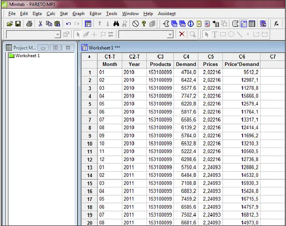
Figure 4 Example for the data of Pareto Analyses
The Food Company is using SAP ERP for the inventory managment and the data is from SAP System. The price of each product is assumed to vary from year to year. As seen above; The data’s time line is between Jan 2010-October 2012 the product’s prices and demands are analyzed by using monthly datas. Prices and demand multiplied for each product and the result is used for the pareto analysis.
Figure 5 Example for the data of Pareto Analyses
One of the main advantages of performing Pareto analysis comes in the form of uncovering the importance of each SKU. A SKU's importance determines the amount of time and dollars allotted to manage the SKU. Companies use different data to determine SKU importance. For the retail company, Pareto analysis typically centers on sales dollars or units. When retail companies use sales data as the Pareto input, the results tell the retail company its top selling and bottom-selling units (Hamlett, K, 2013).
For the manufacturing company is a typical Pareto analysis centers on cost of goods sold. Manufacturers use cost of goods sold (COGS) Pareto analyses to focus on lowering the total cost of more expensive materials (Hamlett, K, 2013). The next big advantage of performing Pareto analysis is determining SKU control. After determining the importance of each SKU, a company can assign the correct inventory control procedures to manage inventory at the SKU level. Not all SKUs require the same type of management. A company may determine that all "A" classed SKUs require weekly replenishment orders and safety stock levels equivalent to two weeks of the SKU's demand. Even within the "A" classed items, different levels of SKU control can exist. Another company might
Price*Demand 1901782 1201593 1048188 703964 581117 539355 159713 Percent 31,0 19,6 17,1 11,5 9,5 8,8 2,6 Cum % 31,0 50,6 67,7 79,1 88,6 97,4 100,0 Ürünler Other 1531 0009 9 1531 0078 2 1531 0268 4 1531 0010 2 1531 0010 1 1531 0010 0 6000000 5000000 4000000 3000000 2000000 1000000 0 100 80 60 40 20 0 P ri ce * D e m a n d P e rc e n t
require that all "E" classed items (Pareto analysis does not have to stop at class "C") get purchased once a year to meet the entire year's demand. The end result of the analysis forms the basis for assigning each SKU an inventory control method that best suits that SKU's importance and the overall goals of the company (Hamlett, K, 2013).
While the standard ABC inventory system works based on the volume of movement, some companies intermix other criteria to monitor specific inventory items. You can classify extremely high-cost inventory items as 'A' items, so you can monitor them more closely. Likewise, you can classify items with extremely long lead times as 'A' items to help prevent ordering delays (Hamlett, K, 2013).
In this research the Pareto is classified for the Cost of Goods Sold and categorized as; “A” is greater than %70, “B” is between %30 and %10, “C” is less than %10.
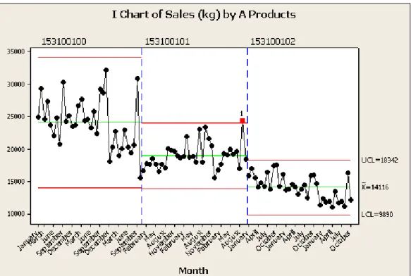
Inventory Turnover for the products which products are classified as A in
Pareto;153100100, 153100101 and 153100102 In 2010 ; 703.806 510.033 = 1,38 In 2011 ; 707.662 456.298 = 1,55 In 2012 ; 524.050 401.681 = 1,31
Figure 6 Sales Quantity Change of A Products between January 2010 and October 2012
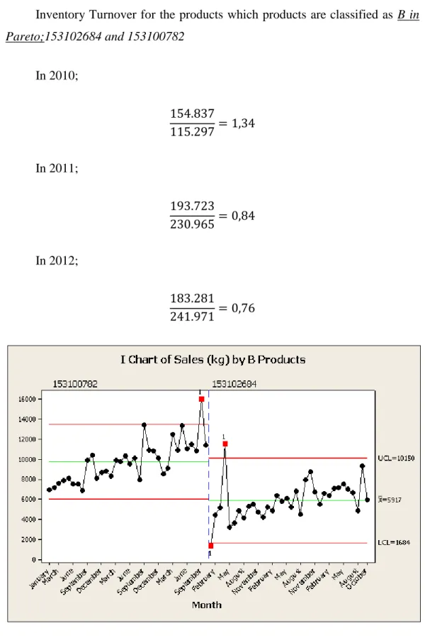
Inventory Turnover for the products which products are classified as B in Pareto;153102684 and 153100782 In 2010; 154.837 115.297= 1,34 In 2011; 193.723 230.965= 0,84 In 2012; 183.281 241.971= 0,76
Figure 9 Stocks Quantity Change of B Products between January 2010 and October 2012
Inventory Turnover for the products which products are classified as C in
Pareto;153100099 and 153102266 In 2010; 102.549 88.836 = 1,15 In 2011; 106.565 83.996 = 1,27 In 2012; 95.160 98.035= 0,97
Figure 10 Sales Quantity Change of C Products between January 2010 and October 2012