Impact of school type on student academic achievement = Okul türünün öğrenci başarısı üzerindeki etkisi

Education and Science

Impact of School Type On Student Academic Achievement

Mehmet Cansız

, Bilgehan Ozbaylanlı

, Mustafa Hilmi Çolakoğlu

Abstract

Keywords

This study aims to investigate the causal effects of school type on the student achievement. Schools type involves two categories: public schools and private schools; whereas student achievement is defined in terms of an overall measure named as Basis for Admission Score (BAS), which is a weighted score reflecting both the grades obtained from courses in each school and the points obtained at nation-wide centralized exams. Factors used as controls in the study include gender of the student, parental attributes (are they alive and live together; their levels of education and occupations), type of the house (own/rent/public housing), separate room of the student, city the family lives in and the level of development of the geographical region. This study utilizes a dataset comprising 3,752,374 secondary school students, which covers all of the student population of Turkish secondary schools within 2014-2016 period. This comprehensive dataset is utilized for the first time in such a study.

At the first step, we present the literature on the effects of school type on academic achievement measured by test scores. This literature can be traced back to 1960’s. On the other hand, a second line of literature, which focuses on the evaluation of causal effects of policies and of programs has progressed swiftly starting from 1980’s and promises an important methodological framework for evaluation of policies and programs in education science. The methodology of this study is designed by bringing together the mentioned two lines of research. Methodology involved the application of regression adjustment, inverse probability weighting, and exact matching techniques in a complementary style in order to ensure the robustness of estimations.

Under the assumptions discussed in detail in the study, we have found that school type has significant impact on student achievement in Turkey. Being a private school student instead of public school student leads to 87 points increase (29.6%) on average in BAS score. It is found that school type has a comparatively larger

School type Public school Private school Student achievement Causal inference Evaluation, regression adjustment Inverse probability weighting Exact matching Doubly robust estimation

Article Info

effect in Turkey compared to other country examples. Based on the findings of the study, a set of research topics are suggested with the objective of improving equality of opportunity in education and of identifying new policies to improve quality of education in public schools.

Introduction

Differences in educational achievement of students studying at different school types are important for families and governments. Families who select private school option invest a serious portion of their family income in this manner. For example, annual fee of private secondary schools in Turkey varies between 22 to 46 times the monthly minimum salary (Ministry of National Education E-School Portal, 2016).

From the perspective of governments, private school system demands well-founded policy decisions. First, private school system is a resource that enable government to share the burden of the national education services. Moreover, they are considered to possess the capacity to increase the overall quality of educational services. Of course, governments also have to regulate and support the services provided by private schools. In particular, governments often subsidize a group of students, such as students from financially restricted families, so that they can be educated at private schools.

Understanding the effects of school type on the student achievement thus is important as it is the very first step to think further about these individual decision and government policy issues. In this study, the target group is secondary school students and their educational achievements. The specific student achievement measure of this study is the BAS score, which stands for the overall score a student achieves at the end of secondary school that she can utilize during the application to high schools. Ranging from 0 to 500 points, BAS score is an amalgamation of the outcomes of centrally-held examinations and the in-the-classroom performance. Beyond being an indicator of educational achievement, BAS score is a decisive measure in the sense that it shapes the future educational path of students. Several prominent high schools adopt BAS as the central admission criteria (Tebliğler Dergisi, 2013).

Investigation of differences in educational achievement in terms of test scores and/or course grades between public and private school students has long been a prolific and sometimes contested research issue. As Hoxby, Caroline and Murarka (2008) argued, to the layman, it is perhaps surprising that researchers highly struggle to come up with an answer to the narrow question: “What is the effect of private schools on the achievement of students who wish to attend them?”.

Abbreviated as “public-private school achievement debate” (Braun, Jenkins, & Grigg, 2006; Peterson & Laudet, 2006), this line of research generally is assumed to start with the study of Coleman et al. (1966). In fact mentioned study was not specifically about public-private debate and its main focus was on reflecting a new perspective on understanding the factors leading to student achievement. Until that date, student achievement was considered to the greater extent an outcome of the quality of the school, which is a function of school resources (Center on Education Policy, 2007). Coleman et al. (1966) controlled for family background characteristics in addition to indicators of schools resources such as expenditures per student, quality of teachers, class size, variety of school facilities, etc. As a striking finding of this pioneering observational study on the student achievement, authors discovered that impact of the size or the variety of resources of the schools on the educational achievement of the

Another important study that scrutinized the educational achievement is provided by Bourdieu (1986) in the sociology field. Emphasizing the close relationship between social background and educational achievement, the author identifies components of the social background as family resources, education levels and occupations of parents, raising up and living in rural or urban areas, and the gender of the student. In this context, social background inherited from the family is the fundamental factor that affects decisions and outcomes related to educational achievement, graduation (or not graduation) from certain schools, studying at rural or urban regions (Bourdieu, 2013). Moreover, social background helps them to do the right thing at the right time in their field and also guide them so that they sense and due prepare for the direction that society tends to incline (Swartz, 2013, p. 11). Bourdieu calls them as born in the game, i.e. who are acquainted to the game since they were born (Bourdieu, 2013, p. 73). Bourdieu, Passeron, & Jean-Claude (2014, p. 16-17, 30-31), in Successors, have studied the university students according to their social background. Social background was analyzed in terms of father’s occupation, and outcomes such as the likelihood of continuing university education, educational achievements, and artistic activities are compared between representatives of various different social backgrounds. Findings indicate a strong association between education and social background. It was found that the likelihood of a child whose father is a top level manager to enter into university is 80 times greater than a child whose father is a farm laborer (Cansız, 2016, p. 85). In sum, according to Bourdieu (2013), social background poses a very significant effect on both the decisions and the outcomes throughout the educational life, especially at the critical junctions of it.

The main subject of this study, the private school effect, are identified for the first time by Coleman, Hoffer, and Kilgore (1982), whose findings indicated a positive private school effect even after socioeconomic status and other key background characteristics of students were taken into consideration. Mentioned study was criticized for being a cross-sectional one, i.e. that it involved data at a single point in time. It might be possible that private school students were already superior in performance before they got into the private school. So the reason for the differential performance was due to this difference in prior-characteristics rather than due a private school effect (Center on Education Policy, 2007).

In order to address mentioned criticisms, Coleman and Hoffer (1987) conducted a longitudinal analysis that involved tracing students throughout 10th _{to 12}th _{grade and they monitored their}

performance trajectory. Findings of the study also indicated a positive private school effect: private school students enjoyed greater performance growth. According to authors, private school students succeeded more number of courses, did more homework, attend more classes and confronts lower number of disciplinary hurdles at the school as compared to the public school students with analogous educational achievement in the previous education levels and with comparable social backgrounds.

Chubb, John, and Terry Moe (1990) integrated data of organizational characteristics of the schools to the Coleman and Hoffer (1987) dataset and found that private school advantage was present and it was associated with much lower numbers of bureaucratic challenges, as well as greater degree of autonomy within private schools. The study found quality of education is not related to teacher salaries, per-pupil spending, or student-teacher ratios. Most significant causes of student achievement were student ability, school organization, and family background, respectively. Bryk, Lee and Holland (1993) studied Catholic schools, which are among prominent private schools in United States, and also found a positive private school advantage, which authors associated to a more coherent academic and social circumstances in that type of schools.

In the study of Center on Education Policy (2007), private school advantage was found to be vanished when supportiveness level of actions and attitudes of parents towards school tasks and issues

whose children were enrolled at private schools possessed characteristics that allows them be more supportive to their children learning challenges. Authors claim that actually this is the reason for the educational achievement gap between the two groups. These parents also carry more ambitious expectations in terms of the educational prospects of their children. Their likelihood of working through the homework with their children is higher. Hence their children receive greater overall support and interactive time from their parents. Those parents are also found to be providing more cultural capital to their children. For example, they go more often to the museums, science-parks or theatres with their parents and more likely to learn to play a music instrument. So, they find ample opportunities to observe and socialize, which create occasions for them to relate what they learn at class to real life experiences as well as urge them to elaborate on these with their parents and friends.

Varied findings are reported about the effects of school type on student achievement. Center of Education Policy (2007) and Abdulkadiroğlu et al. (2009) did not find statistically significant impact, but Angrist et al. (2011) found that studying at a private school has increased math scores by 0.2 standard deviations. Frenette and Chan (2015) also found 8% increase for private school students. On the other hand Chingos and West (2015) ended up with a slightly negative effect of 0.041 standard deviations.

In the context of the studies carried out in Turkey, Berberoğlu, Giray and Kalender (2005) aimed to identify how the academic achievement vary according to different school types and geographical regions. Apart from a few prestigious public high-schools, the achievement difference was found to be the largest among OECD countries. The achievement differences related to living in different regions were comparatively smaller. Alacacı and Erbaş (2010) utilized PISA 2006 study, which includes 4942 students from Turkey in order to study the level of inequality among schools and found that the achievement levels of Turkish schools represent the largest variation among OECD countries. Sulku and Abdioğlu (2015) utilized TIMMS 2011 data to evaluate the factors affecting achievement for primary schools students and found that the average mathematics score of public school students was 446.6 compared to the private schools students’ average of 607 after controlling for several background characteristics. Borkan and Bakis (2016) utilized the data of 184.587 secondary-school students to investigate the role of school and student factors for academic achievement. Authors concluded that 18 per cent of the variation was due to intra-school differences whereas the remaining variation was due to within-school factors. However, mentioned study did not use a school type variable, which indexes public and private schools separately.

Reçber, Işıksal, and Koç (2018) investigated if the achievement in mathematics of and the student attitude towards mathematics differ between public and private schools found that levels of achievement did not differ significantly but private school students’ attitudes are more positive. Mentioned study faced some data limitations since only 13 school in the district city Ankara were sampled and sampling was not random since the authors selected the schools which are most suited to authors’ easy of access. Arslan, Satıcı, & Kuru (2006) evaluated the effectiveness of private and public schools based on the perceptions of teachers by using data consisting 190 teachers from 3 private and 3 public schools in Gebze-Kocaeli in Turkey and concluded that private schools were more effective in terms of the following five criteria: school inputs, school atmosphere, school infrastructure, teaching/learning processes, and the outcomes of this processes. Mohammadi, Akkoyunlu Pınar, and Şeker (2011) investigated the factors important for the students with highest levels of achievement by utilizing a sample of 810 students, found that the type of school played a significant role however the family factors such as the level of education and income of parents did not play a significant role for his

On the other hand, our study has a significant advantage of covering the whole student population of secondary school students, which covers over 3.7 million students. The opportunity to utilize the whole population data prevents from representability and sampling related problems and ensures statistical power. In observational studies, the most critical role is played by the study design in order to achieve robust inferences (Imbens & Rubin, 2015; Sekhon, 2007). In this context, the other objective of this study is to present the methodological approach which ensures the robustness of the findings. Robustness requires the exposition of the assumptions foreseen the methodology fully as well as providing the rationale that they are met by the data availability and the effectiveness of the study design. In overall, it is observed that previous studies have not put sufficient emphasis on elaboration of the validity of assumptions and on assessment of robustness of the results. Our study aims to account for the validity of the assumptions and robustness. In addition, this study takes a different stance than the previous studies in Turkey by its focus on an approach, which aims to isolate the causal effect of a unique policy variable, which is here the school type. If we do not isolate the causal effect of a policy variable, then the policies derived from findings of our study would impose risks of being irrelevant or ineffective. In this context, our study also aims to establish an example for implementation of casual inference approach and techniques for the field of education policy research in Turkey. In this context, the implementation of three casual inference techniques -regression adjustment, inverse probability weighting, and exact matching- in a complementary approach is also a contribution of this study to the implementation of causal inference.

On the other hand, the prominent aspect of observational studies is the use of control variables in order to eliminate the bias in estimates, so which control variables to involve is a core question of the observational study design. Findings of the previous literature provide important indications for this purpose. The findings of Bourdieu (2013), Bryk et al. (1993), Coleman et al. (1966) and Center on Education Policy (2007) provide examples from this perspective. There are numerous studies conducted in Turkey as well. In this context, Arı (2007), Sarıer (2010), Şengönül (2013) and Yavuz, Odabaş, and Özdemir (2016) draw attention to the relation between the academic achievement and socioeconomic status. Findings of OECD (2010) indicated that Turkey was in the third rank in OCED member countries according to the interdependency between academic achievement and socioeconomic status. According to Kalaycıoğlu, Çelik, Çelen and Türkyılmaz (2010), socioeconomic status of a household depends on level of education of family members, average monthly income, occupations and workplaces, home or automobile ownership, and means and facilities at the home.

Şengönül (2013) draw attention to two theories and their implementations in term of the relation between socioeconomic status and academic achievement: Family Stress Model and Family Investment Model. According to Family Stress Model (Conger et al., 2002), as a result of the low levels of income relations between family members deteriorate, parents show less interest on their children and exhibit demoralizing behavior which results in provision of little to no help in their educational process. From the perspective of Family Investment Model (Brooks-Gunn, Klebanov, & Liaw, 1995), families with more income provide more financial, social and cultural capital to their children. Findings of İmamoğlu (1987) and Kağıtçıbaşı and Ataca (2005) from Turkey can be regarded as examples in the context of Family Stress Model (Şengönül, 2013). Highlights from mentioned studies indicated that poor parents show less interest in their children’s education life, and while they expect gratitude from their children wealthy parents expect less gratitude and provide more autonomy to their children. Examples for Family Investment Model (Şengönül, 2013) involve Ataman and Epir (1972), and Yağmurlu, Çıtlak, and

especially the mother’s use of a limited vocabulary and excessive punishment action on the children have implications in terms of academic achievement of the child. Other factors in this context include less amount of education materials procured by the parents, less attention per child in the crowded families and the lower attention of the child during dealing with homework because of the crowded home atmosphere as a result of high number of siblings in large families.

In their study focusing on students of a primary school located in a lower socioeconomic status, Yelgün and Karaman (2015) found that the major factors reducing academic achievement are low education levels of parents, low levels of family income, lack of separate room or study environment of the child, mandatory outdoor working of the children because of lack of adequate income, working of the father in another province, lack of father’s regular job and income, and high number of siblings. On the other hand, the fact that the district of the family is located far away from the city center or at a rural area, and the lack of role models in the district are determined in terms of environmental factors affecting academic achievement. Engin-Demir (2009) found the most important factors as the level of education of the father, family’s ownership of the home, and teacher-to-student ratio. According to Güvendir (2014) on the other hand factors affecting Turkish skills are gender of the student, level of education of the father, number of books owned, time allocated to reading, receiving private tutoring, the ratio of girls in the school, average size of the class and the location of the school.

Yayan and Berberoğlu (2004) and Ceylan and Berberoğlu (2007) found by using TIMMS 1999 data that the factors affecting science and mathematics achievement are the perception of the student of success and failure, socioeconomic status of the family, education levels of the parents, and student-centered activities. Avşar and Yalçın (2015), based on PISA 2009 data found that students whose fathers have graduate degrees had better reading skills. Moreover, they also observed that children who received pre-school education also had improved reading skills, and they suggested that sending the children to a pre-school is a function of high-enough income levels and the fact that the mother was working. In terms of other studies utilizing PISA 2009 data, Gürsakal (2012) found that gender, age, and education levels of parents are the factors that significantly associated with science and mathematics literacy; and Özdemir and Gelbal (2014) found that socioeconomic status of the family and amenities to study at home are important for academic achievement. Koğar (2015), using PISA 2012 data (OECD, 2010), identified that the factors that affect mathematics literacy are socioeconomic status of the family, gender of the student and the time allocated to learn mathematics. Özbay (2015) is another study utilizing PISA 2012 data to find that the geographical region is an important factor for academic achievement.

The prominent aspect of above-mentioned studies is the fact that the type of the school (public/private) in not controlled for when assessing the relation between several background factors and the academic achievement. One of the contributions of our study is to control for this important aspect.

On the other hand, studies on differences between private and public schools regarding educational achievement do not solely involve observational approach. Numerous experimental and quasi-experimental methods have also been employed. However, there are important tradeoffs involved in choosing one empirical approach over another (Ackerman and Egalite, 2015).

Experimental approach is often regarded as the gold standard methodology for identifying causal effect of private schools that hold admission lotteries. In this setting, treatment and control groups are generated by chance. However, lottery-based studies can only occur when demand of applicants is greater the capacity supply of the private school. Experimental studies typically compare students who have won and lost admissions lotteries at popular charter schools. This identification strategy can yield unbiased estimates of the local average treatment effect for oversubscribed schools, yet such studies can potentially suffer from problems of external validity, as oversubscribed charter schools might differ from undersubscribed charters. As a result, it is unsurprising that the vast majority of experimental studies have been conducted in population-dense urban centers (Hoxby & Rockoff, 2004, Abdulkadiroğlu et al., 2009; Dobbie & Fryer, 2011).

Similarly, in quasi-experimental studies, reliable and valid instruments are hard to find, particularly in large-scale evaluations of charters across multiple locales. Observational studies, meanwhile, permit the researcher to include most charter students in a region, thereby enhancing their external validity. Yet these studies may have weak internal validity because of the challenges associated with establishing an appropriate counterfactual (Abdulkadiroglu et al, 2009).

Peterson and Laudet (2006) argues that there is a pool evidence that well-implemented observational methods can produce unbiased estimates of charter effects, even in the absence of random assignment. Abdulkadiroğlu et al. (2009), Angrist et al. (2011), , and Fortson, Verbitsky-Savitz, Kopa, and Gleason (2012) compare impact estimates generated from experimental data to those from alternative, non-experimental methods to judge how close the estimates produced by an observational approach come to replicating the unbiased experimental estimates. All three studies report promising findings supporting the validity of observational methods for estimating charter effectiveness.

Hence our specific research question is as such: What is the average causal effect on the BAS score of studying at a private school compared to studying at a public school for secondary school students in Turkey? This study attempts not to be restricted to building a predictive model to predict a BAS score conditional on some set of characteristics related to the student and other relevant factors; instead the main objective is to identify the average causal effect of studying at private schools compared to studying at public schools as precisely as possible under a set of appropriate assumptions. Hence the study will set out with setting the framework of causal inference. In the following, theoretical foundations of three different methods that based on potential outcomes framework will be introduced. As precision of any causal inference effort is bounded with the appropriateness of the assumptions and limitations of data, detailed account for assumptions and limitations is presented afterwards. Three main causal inference approaches -regression adjustment, inverse probability weighting, and exact matching- will be employed in a manner supplementing each other to estimate the causal effect as robust as possible.

The types of estimators estimated in the analysis section are Average Treatment Effect (ATE), Average Treatment Effect on Treated (ATET), and Potential Outcome Means (POMs) related to ATE and ATET. After the theoretical background on causal inference is set forth, mentioned estimators will be defined in detail and interpreted in the light of findings.

Method

This study aims to estimate the causal effects of school type on the student achievement. Schools type involves two categories: public schools and private schools; whereas student achievement is defined in terms of an overall measure named BAS score (Basis for admission score), which is a weighted score reflecting both the grades obtained from courses in each school and the points obtained at nation-wide centralized exams. Factors used as controls in the study include gender of the student, parental attributes (are they alive and live together; their levels of education and occupations), type of the house, separate room of the student, city the family lives in and its level of development. Study utilizes a dataset comprising 3,752,374 secondary school students, which covers all of the student population within 2014-2016 period. This comprehensive dataset is utilized for the first time. In the context of the below subsections, first the aspects of the dataset is summarized, then casual estimation and its notation, which form the theoretical background of the methodology is set forward. Following section estimation methods are introduced.

Data

This study relies on the administrative dataset provided by the Ministry of National Education of Turkey. Mentioned dataset includes information about the BAS Score and the School Type of all of the 3,752,374 students dispersed over the years between 2014 and 2016. Dataset also includes information about covariates listed at Table-1. As you can see, nearly of the covariates are subjected to no-response to some extent; but generally the ratio of response is substantially higher. Overall we can assert that we are utilizing a close-to-population level of data in our analysis.

Table 1. Data Summary

Variable Variable Type Values Response No Response

YEP Score Outcome Continuous in points 3,752,374 0

School Type Treatment Public, Private 3,752,374 0

Gender of Student Covariate Boy, Girl 3,751,394 980

Father's Life Status Covariate Alive, Not Alive 3,733,213 19.161

Mother's Life Status Covariate Alive, Not Alive 3,727,549 24.825

Parent's Marital Status Covariate Married, Divorced 3,752,374 0

Father's Education Covariate Up to Primary, Secondary/High, Undergrad, _Master/PhD 3,219,580 532.794 Mother's Education Covariate Up to Primary, Secondary/High, Undergrad, _Master/PhD 3,205,073 547.301 Father's Occupation Covariate Not Working, Non-Public Worker, Public _Worker 3,231,778 502.596 Mother's Occupation Covariate Not Working, Non-Public Worker, Public _Worker 3,209,181 543.193 Resident Type of Family Covariate Rent, Own House, Public Quarter 3,557,865 194.509

Student's Own Room Covariate No Own Room, Own Room 3,559,774 192.6

City Covariate 81 different cities in Turkey 3,748,878 3.496

Year Covariate 2014, 2015, 2016 3,752,374 0

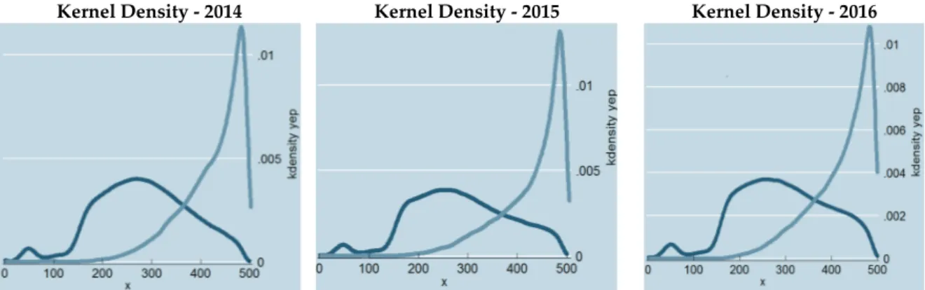
BAS score is a continuous variable varying between 0 and 504.44 points. Its mean is 294.07 and standard deviation is 100.49. As expected from a standardized test, its Kernel distribution is very similar among the 3-year period taken into consideration in the analysis. Dark blue line represents kernel density of public school students and light blue line represents the Kernel density of private school students (Kernel distribution let us present our data without any need for any functional form

restrictions or parametric assumptions. It is similar to Histogram often used, but it also allows for continuity whereas histograms do not (Zuccini, 2003). Population level average of the BAS scores of private school students is 424.20 and it is considerably higher than the population level average of BAS scores of public school students, which is 287.85.

Kernel Density - 2014 Kernel Density - 2015 Kernel Density - 2016

Figure 1. Kernel Densities of BAS Scores for covered period Causal Inference

This study implements causal inference techniques to identify the average causal effect of studying at private school on educational achievement. Causal inference focuses on comparisons of different treatments applied to the same units; hence it relies on counterfactual interpretations. It differs in this sense from predictive inference, which concentrates on comparisons between different units (Gelman & Hill, 2007). Approaches like Ordinary Least Squares (OLS) that commonly used for predictive inference can also be used for causal inference; but counterfactual interpretation requires substantially stronger assumptions compared to predictive interpretation. Examples of use of OLS based approaches for causal inference are provided in this study. Moreover, several specialized methods have also been developed for causal inference. Regression adjustment estimator, inverse probability weighting estimator and exact matching estimator implemented in this study are examples of such methods.

The most naive estimator for the average effect of private school on educational achievement would involve the straightforward comparison of the average BAS score of private school students and average BAS score of public school students in the population. As we have access to whole population data in terms of individual BAS scores, we can easily do this. But, can we consider this as an unbiased estimate? The answer depends on the answer to a different question: Are these two groups comparable? One of the core concepts of the causal inference is the treatment status, which is the variable indicating if a certain individual is subject to the intervention or not. For example in this study treatment status is zero for the students enrolled in public schools and is one for the students enrolled in private schools. The group of students whose treatment status is one is named as the treatment group, and group of students whose treatment status is zero is named as the control group. The core objective of randomized studies is obtained balance in distributions of student characteristics between treatment and control groups. When mentioned balance is achieved, two groups would be comparable with respect to their baseline characteristics and would be different only in terms of their treatment status. It is not of any importance if these characteristics were observable or unobservable; or that they were measurable or not measurable; if there are enough number of observations, all those characteristics

In contrast, subjects in observational studies, such as in this study, are not necessarily randomly assigned to the treatment group or to the control group, since the researcher has no control over the assignment of the treatment. Hence discrepancies in terms of outcomes of two groups might be partly related to the differences in baseline characteristics if the treatment status is also affected by these baseline characteristics. In that case, participants would self-select themselves into the specific treatment status favored by their characteristics. This self-selection bias can be severe.

Baseline characteristics emphasized above, which both affect the level of the outcome variable and the status of treatment variable are named as confounding covariates. If unadjusted for, confounding variables lead to biased estimates of the treatment of interest. Besides, if there is no correlation between the treatment and the suggested confounder or there is no correlation between the outcome and the suggested confounder, then the variable is not a confounder because there will be no bias. If a variable is not a confounding variable, then we need not to take it into consideration that variable in the causal inference context. Concern about R2 _{are also at most secondary here because we}

are not interested in explaining the dependent variable as much as possible. What we are interested in essence is to isolate the causal effect of the treatment variable, to the extent we could.

Observational studies aim to deliver comparable groups that are valid under a set of identifying assumptions. As we will discuss in the following section, one of those assumptions suggests that the treatment can be regarded as almost randomly assigned after conditioning on the set of all confounding observable variables. This is not directly testable as it implicitly suggest that there are no remaining unobservable confounders as well. Hence the findings based on the explicit part of the assumption need to be substantiated by the convincing deliberations of the researcher on the implicit part of the assumption.

Potential Outcomes Framework

Potential outcome notation suggested by Rubin (1974) provides the building blocks for causal inference. Denote D as the indicator of treatment assignment, it is equal to 1 if for treated individuals and is equal to 0 for the individuals in the control group. Let us define Y0i and Y1i for individual i as the

potential outcomes. These represent counterfactuals for individual i: Y0i is the outcome if the individual

were to receive the treatment and Y1i is the outcome if the individual were not to receive the treatment.

The difference between these two potential outcomes would be equal to the causal effect of treatment on individual i. However, we can observe only one of these potential outcomes; we observe Y1i if the

individual i is treated or Y0i if the individual i is not treated. In Holland (1986)’s words, this is the

fundamental problem of causal inference. So we can also consider causal inference as a challenge related to a missing data problem. Potential outcome framework do not solve this missing data problem at the individual level, but paves the way for conducting causal inference at the distribution level.

Let Y0 be the vector of potential outcomes in the absence of treatment of all individuals that we

are interested with and let Y1 be their vector of potential outcomes under the treatment. The distribution

of Y0 is the hypothetical distribution of outcome if all individuals were not treated, and distribution of

Y1 is the hypothetical distribution of outcome if all individuals were treated. In this potential outcomes

framework, average causal effect η is defined as: η = E(Y1) - E(Y0)

Potential outcomes framework enables formalization of η, and hence makes possible to produce causal statements by the utilization of observational data. What we actually observe is the outcome Y, D and X. Here X is the vector of covariates that logically and temporally proceed the treatment assignment and hence are not influenced by the treatment assignment. However, we need to identify E(Y1) and E(Y0) to identify η. As the first step, we relate the observed outcome Y to counterfactual

potential outcomes Y0 and Y1 as below:

Y = Y(D) = D ⋅ Y1 + (1- D) ⋅ Y0= �Y_Y0 if D = 0

1 if D = 1 (1)

We also observe the average outcome level in the treatment and control groups in the sample, which are E(Y|D=1) and E(Y|D=0), respectively. From (1) we can conclude that E(Y|D=1)=E(Y1|D=1)

and E(Y|D=0)=E(Y0|D=0). However, these are not the same with what we need to know, i.e. E(Y1) and

E(Y0).

By design, randomized controlled trials manipulates treatment assignment D to make it random. So we can conclude for such studies that (Y0, Y1) ‖ D; i.e. potential outcomes are statistically

independent from treatment assignment. In this case E(Y1|D=1) becomes equal to E(Y1), and E(Y0|D=0)

becomes equal to E(Y0). This means that we can use the sample average of treatment group and the

sample average of the control group to identify the average treatment effect; taking directly their difference is sufficient.

In an observational study, on the other hand, because the researcher cannot manipulate the treatment assignment D to make it random, we cannot guarantee that potential outcomes are statistically independent of the treatment assignment. In they are not, E(Y1|D = 1) ≠ E(Y1) and E(Y0|D =

0) ≠ E(Y0) will hold, which means we cannot use sample averages of two groups for estimating η. Hence,

we would need further identifying assumptions, which are discussed in the following section.

Identifying Assumptions

Rosenbaum and Rubin (1983) suggest that conditional on X, we can assume potential outcomes to be statistically independent from treatment assignment, i.e. (Y0,Y1) ‖ D|X, if it is true that X involves

all of the confounding covariates. They call this as ignorable treatment assignment assumption. If this assumption is valid for our study at hand, then E(Y0) and E(Y1) can be identified from what we observe

in the sample as follows:

Ex {E(Y|D = 1, X)} = Ex {E(Y1|D = 1, X)} = Ex {E(Y1|X)} = E(Y1) (2)

Ex {E(Y|D = 0, X)} = Ex {E(Y0|D = 0, X)} = Ex {E(Y0|X)} = E(Y0) (3)

For identification we need one more key assumption, known as overlap assumption, which ensures that the number of observations in treated and control groups to be nonzero for each X=x. (Cameron & Trivedi, 2005). Overlap assumption requires that:

0 < Pr(T = 1|X = x) < 1 ɏ x.

Main identifying assumption of this study, strongly ignorable treatment assignment (Rosenbaum & Rubin, 1983) is the combination of the ignorable treatment assignment assumption and the overlap assumption. Overlap assumption guarantees that E[Y1 – Y0|X=x] is identified for all X=x. Ignorable

treatment assignment assumption takes care of the rest as follows:

η (x) = E(Y1) - E(Y0) = E[Y1|X = x] − E[Y0|X = x] (4)

= E[Y1|D = 1, X = x] − E[Y0|D = 0, X = x]

= E[Y|D = 1, X = x] − E[Y|D = 0, X = x]

Regression Adjustment

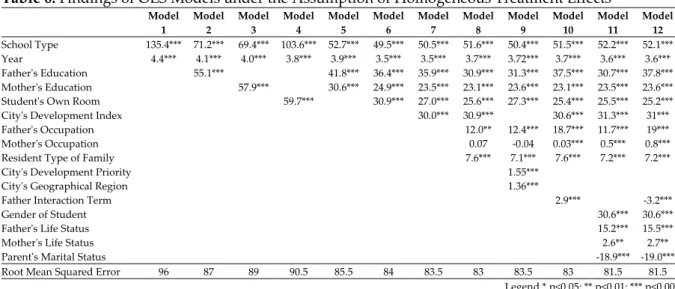
In this section three regression based approaches will be introduced. The first approach implements OLS under the assumption of homogeneous treatment effects. The second approach again implements OLS, but this time under the assumption of heterogeneous treatment effects. The third approach implements Regression Adjustment (RA) estimator based on Cattaneo (2010) and Cattaneo, Drukker, and Holland (2013).

OLS under homogeneous treatment effect assumption assumes that the treatment effect is the same for all individuals irrespective of their other characteristics.

As shown in the previous section: η

= E{

Y= β0 + α⋅D + X/βX + ε

E(Y|D, X) = β0 + α⋅D + X/βX

E(Y|D=1, X)-E(Y|D=0, X) = β0 + α (1) + X/βX - β0 – α (0) - X/βX = α

η = E{E(Y|D=1, X)-E(Y|D=0, X)} = E{α} = α

Thus we can estimate η directly by fitting above OLS model.

OLS under heterogeneous treatment effect assumption assumes implicitly that the difference in the treatment effect can differentiate among individuals based on their differentiated characteristics. In order to handle heterogeneous effects, our model needs to also involve the interaction terms between the treatment variable and each of the confounding covariates. Suppose that the true model involving mentioned interaction terms is:

E(Y|D, X) = β0 + αD + X/βX + DX/ψ

E(Y|D=1, X)-E(Y|D=0, X) = β0 + α (1) + X/βX + (1)X/ψ - β0 - α (0) - X/βX -(0)X/ψ = α + X/ψ

So η= E {E(Y|D=1, X)-E(Y|D=0, X)} =E { β0 + X/ψ} = α+ X/ψ

As seen, we can obtain an estimate of causal effect by estimating the above model as it will provide estimates of αandψ in addition to X, which is already observed.

The final approach in this section implements regression adjustment estimator based on Cattaneo (2010) and Cattaneo et al. (2013). It differs from OLS based estimators described above in two aspects: It is an exactly identified generalized method of moments (GMM) estimator and involves two steps: In the first step, separate linear regression models are fitted with the observed data for the each treatment group, while controlling for the set of confounding covariates.

We have shown that before:

η (x) = E(Y1) - E(Y0) = E[Y1|X = x] − E[Y0|X = x] = E[Y1|D = 1, X = x] − E[Y0|D = 0, X = x]

= E[Y|D = 1, X = x] − E[Y|D = 0, X = x]

First step of RA estimator produces E[Y|D = 1, X] and E[Y|D = 0, X] as first corresponds to the line for the fitted values of the regression of outcome on X for D=1; and the latter corresponds to the line for the fitted values of the regression of outcome on X for D=0. E[Y|D = 1, X] informs us on E[Y|D = 1,

Second step differentiates the above two expectations for each X=x and then averages out for all x as we shown before to estimate ATE:

η=

E

[

] = E

{

Propensity score constitutes the fundamental concept of IPW estimator. The propensity score is defined as the probability of selection into treatment conditional on some set of observed covariates:

e(X) = Pr(D=1|X)=E[D|X]

Rosenbaum and Rubin (1983) have shown that if ignorability of treatment assignment assumption holds given X, then ignorability of treatment assignment assumption would also hold given propensity score e(X). Proof can be found in Imbens (2004, p. 8).

(

)

|

IPW method assigns weights to the individuals by using as weights the inverse of the propensity score, i.e. the probability of being in the observed treatment group in order to make treatment assignment independent of covariates that we condition on.

If we remember from previous sections, causal effect, i.e. average treatment effect is: η = E(Y1) - E(Y0)

Below equations show how IPW estimator identifies η:

E[Y1] = E[E(Y1|X)] = E �e(X)⋅E(Y_e(X)1|X)�= E �E(D|X)⋅E(Y_e(X) 1|X)�= E �E �D⋅Y_e(X)1� |X�= E �D⋅Y_e(X)1�= E �_e(X)D⋅Y�

E[Y0]=E[E(Y0|X)]=E �(1−e(X))⋅E(Y_1−e(X)0|X)�=E �E(1−D|X)⋅E(Y_1−e(X) 0|X)�=E �E �(1−D)⋅Y_1−e(X)0� |X�=E �(1−D)⋅Y_1−e(X)0�= E �(1−D)⋅Y_1−e(X)�

As η = E[Y1] – E[Y0] = E[Y(1) – Y(0)]; above two equations together imply: η = 𝐸𝐸 �_e(𝐗𝐗)D⋅Y− (1−D)⋅Y_{1−e(𝐗𝐗)}�

Estimator given below enables us to infer from our data (Horvitz & Thomson, 1952): ῆ = _N1 ∑ �Di ⋅ Yi e(𝐗𝐗i) − (1−Di)⋅ Yi 1−e(𝐗𝐗i)� N i=0

As e(⋅) above stands for the true propensity score and is rarely known, we often need to use estimated propensity score ê(⋅) (Imbens, 2004). Hirano, Imbens, and Ridder (2003) have shown that use of estimated propensity score is even better than using true propensity score in terms of large sample efficiency. Based on the estimated propensity score, ê(Xi),we end up with the inverse probability

weighting estimator as below (Imbens, 2004): ῆ = ∑ Di ⋅ Yi ê(Xi)/ ∑ Di ê(Xi) N i=0 N

i=0 – ∑ Ni=0 (1−D_1−ê(Xi) ⋅ Y_i)i/ ∑Ni=0_1−ê(XDi_i)

Matching

Matching is a nonparametric method that at first constructs a matched group for the treated group based on the similarities in terms of confounding characteristics, and then compare their average outcomes at the second step (Rosenbaum & Rubin, 1983; Ho, Imai, King, &.Stuart 2007). Exact matching estimator ῆ employed in this study is such that (King & Nielsen, 2016, p. 4):

ῆ = meaniЄ{i |Di=1}[Yi-Ŷi(D=0)] where Ŷi(D=0) = meanjЄ{ j |Xj=Xi,Di=1,Dj=0}Yj

given E[Y0 | X=x] = E[Y0 | D=0, X=x] = E[Y | D=0, X=x] under strong ignorability;

Results

As mentioned in the section titled Data, population level average of the BAS scores of private school students is 424.20 and it is considerably higher than the population level average of BAS scores of public school students, which is 287.85.

If the treatment assignment could be considered as random and independent from the potential outcomes, as in randomized experiment studies, the treatment and control groups would be balanced in terms of other important characteristics. In this case we can use the difference between average outcome levels of treatment and control variables as the estimator for population level average treatment effect since the only different characteristic remained between the two groups that we can attribute the effect on outcome is the school type. So in that case, 424.20-287.85 = 136.35 points would be the population level average treatment effect, which is quite sizeable.

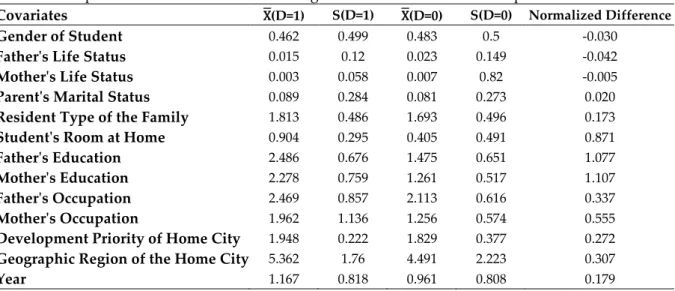
As this study is an observational one instead of a randomized experiment, assignment mechanism is not necessarily random. Because of self-selection into treatment, other important characteristics may not be balanced, which can potentially bias our estimates. Imbens and Rubin (2007) suggest the use of normalized difference for each covariate to assess the imbalance between treatment and control groups.

Normalized difference = X�(D=1)− X�(D=0)

�S2_(D=0)+S2_(D=1) (S2(D=w) is the sample variance for group w)

We can observe from Table-2 that indeed several covariates are indeed unbalanced as normalized difference is far from being equal to zero; for some variables it is even around one. This is an indicator for sizeable levels of bias introducing self-selection, which we need to correct for.

Table 2. Comparison of Covariate Values among the Treated and Control Samples

Covariates X(D=1) S(D=1) X(D=0) S(D=0) Normalized Difference

Gender of Student 0.462 0.499 0.483 0.5 -0.030

Father's Life Status 0.015 0.12 0.023 0.149 -0.042

Mother's Life Status 0.003 0.058 0.007 0.82 -0.005

Parent's Marital Status 0.089 0.284 0.081 0.273 0.020

Resident Type of the Family 1.813 0.486 1.693 0.496 0.173

Student's Room at Home 0.904 0.295 0.405 0.491 0.871

Father's Education 2.486 0.676 1.475 0.651 1.077

Mother's Education 2.278 0.759 1.261 0.517 1.107

Father's Occupation 2.469 0.857 2.113 0.616 0.337

Mother's Occupation 1.962 1.136 1.256 0.574 0.555

Development Priority of Home City 1.948 0.222 1.829 0.377 0.272

Geographic Region of the Home City 5.362 1.76 4.491 2.223 0.307

If we revisit the criteria for assessment of a confounding covariate; to be employed as a confounding covariate and thus controlled for, a covariate needs to be (Imbens & Rubin, 2015, p. 265-66):

1. A confounding covariate should be correlated with both the outcome variable and the treatment variable at the same time. If there is no correlation between the treatment and the suggested confounder or if there is no correlation between the outcome and the suggested confounder, then the variable is not a confounder because there will be no bias. The degree of this correlated is also important; more emphasis shall be put on covariates with higher double-correlation.

2. We should not employ post-treatment variables as confounding covariates. Post-treatment variables are measured after or at same time with the treatment, are themselves affected from the treatment or are consequences of the treatment. We need to be sure that confounding covariates chosen have to be pre-treatment variables, which are logically prior to the treatment and most importantly cannot be affected from the treatment.

In terms of the first condition, correlations between outcome, treatment and potential confounding variables are presented in Table-3. Father’s education, mother’s education, and existence of student’s own room at home are the three potential confounding variables that have highest double-correlation levels. Father’s occupation, mother’s occupation, geographical region of the school, and development priority of the home city follows them as the second group in terms of double-correlations. Year and resident type of the family constitutes a third group in that sense. These three groups are suitable for being selected as confounding covariates. Father’s life status, mother’s life status, and parent’s marital status are almost not correlated with neither the outcome nor the treatment variable. Gender has a considerable correlation level with the outcome variable but almost have non-existing correlation with the treatment variable, which disqualifies it from being a confounding covariate.

Table 3. Correlations between Outcome, Treatment and Potential Confounding Variables

YEP S co re Sc hool T yp e G ende r Fa th er' s Li fe Sta tu s M ot he r's Li fe Sta tu s Pa re nt 's Ma ri ta l S ta tu s Fa th er' s Edu ca tio n Mo th er 's Edu ca tio n Fa th er' s Oc cup at ion Mo th er 's Oc cup at ion Re si de nt Ty pe o f F am ily St ude nt 's Ow n Room G eo gr ap hi ca l Re gi on D ev el op m en t Pri ori ty Ye ar YEP Score 1.000 School Type 0.272 1.000 Gender 0.160 -0.010 1.000

Father's Life Status -0.015 -0.009 0.002 1.000

Mother's Life Status -0.012 -0.005 0.000 0.017 1.000

Parents' Marital Status -0.017 0.007 0.005 0.389 0.134 1.000

Father's Education 0.444 0.310 0.006 -0.021 -0.011 0.018 1.000

Mother's Education 0.400 0.366 0.005 -0.016 -0.010 0.076 0.582 1.000

Father's Occupation 0.283 0.116 0.001 -0.020 -0.006 -0.023 0.485 0.307 1.000

Mother's Occupation 0.204 0.231 0.000 -0.005 -0.005 0.077 0.288 0.465 0.234 1.000

Resident Type of Family 0.063 0.050 -0.003 0.001 0.002 -0.059 0.043 0.024 0.055 0.027 1.000

Student's Own Room 0.334 0.197 0.010 -0.016 -0.010 0.031 0.382 0.373 0.230 0.176 0.067 1.000

Geographical Region 0.135 0.073 0.002 -0.013 -0.009 0.047 0.107 0.144 0.024 0.057 -0.075 0.217 1.000

Development Priority 0.155 0.084 0.003 -0.014 -0.010 0.057 0.141 0.184 0.045 0.074 -0.103 0.247 0.807 1.000

Table 4 presents detailed account of distributions of outcome and treatment levels with respect to different values of each covariate. Apart from reflecting the same information of Table-3 in a different and more detailed format, Table 4 provides the perspective of the potential outcome framework for assessment of confounding covariates. As an illustration, let us analyze the case for father’s education.

In order to set an example on how to interpret the information in Table-4, detailed explanations will be provided by using father’s education covariate. Same style of explanation is also valid for the other covariates. In terms of father’s education, ratio of treated students to overall population increases with each incremental increase in education level. Whereas only 0.77% of students whose fathers’ education level is up-to primary school are enrolled to a private school, this increases to 4.41% for students whose fathers’ education level are secondary and high school level of education, to 21.91% for students whose fathers’ education level is undergraduate, and to 42.60% or students whose fathers’ education level are masters or PhD. This indicates a strong correlation between the level of education of father and the odds of enrollment of the children to a private school. This is also an evidence for the case that fathers with higher level of education have a significantly higher tendency to enroll their children to a private school. In other words, they self-select their children to a private school at a higher rate as their level of education becomes higher. As discussed before, self-selection like this would mean that the direct comparison of sample means of treated and control groups would lead to bias if father’s education level is also correlated with the BAS score.

Another important observation from Table-4 is the fact that BAS score increases with each incremental increase in the level of father’s education both for the treated and control groups. In the treated group, average BAS score of private school students whose fathers’ level of education is up-to primary is 377.21, this increases to 402.59 for private school students whose fathers’ level of education is secondary or high school, to 443.97 for private school students whose fathers’ level of education is undergraduate, and to 453.65 for private school students whose fathers’ level of education is masters or PhD. In the control group, average BAS score of public school students whose fathers’ level of education is up-to primary is 266.26, this increases to 320.19 for public school students whose fathers’ level of education is secondary or high school, to 387.32 for public school students whose fathers’ level of education is undergraduate, and to 394.74 for public school students whose fathers’ level of education is masters or PhD.

Table 4. Distributions of Outcome & Treatment Levels with Respect to Different Values of Covariates

Population Treatment: Private School Control: Public School

# of Obs. % of Obs. _Mean YEP Score _Std.Dev. Ratio of _Treated Ratio of _Control # of Obs. % of Obs. _Mean YEP Score _Std.Sap. # of Obs. % of Obs. _Ortalama YEP Score _{Std. Sap.}

Gender of Student Boys Girls 1,943,703 1,807,691 51.80 48.17 279.15 310.16 99.87 98.63 4.73 4.37 95.27 95.63 79,037 91,974 46.19 53.75 432.02 417.62 61.13 70.10 1,728,654 1,851,729 48.27 51.71 304.60 272.27 96.05 96.40

No Response 980 0.03 217.39 109.55 11.84 88.16 116 0.07 321.25 102.02 864 0.02 203.44 102.88 Father's Life Status Alive 3,650,334 97.28 294.76 100.43 4.60 95.40 167,952 98.14 424.57 66.40 3,482,382 97.24 288.50 97.51 Not Alive 82,879 2.21 276.03 97.62 2.99 97.01 2,482 1.45 409.04 67.93 80,397 2.24 271.92 95.49 No Response 19,161 0.51 241.76 102.80 3.62 96.38 693 0.40 389.01 86.95 18,468 0.52 236.24 99.18 Mother's Life Status Alive 3,702,787 98.68 294.44 100.44 4.57 95.43 169,128 98.83 424.52 66.36 3,522,659 98.67 288.21 97.53 Not Alive 24,762 0.66 265.07 97.92 2.31 97.69 571 0.33 407.90 72.93 24,191 0.68 261.70 95.90 No Response 24,825 0.66 268.01 101.81 5.75 94.25 1,428 0.83 393.10 79.54 23,397 0.66 260.38 97.98 Parents'

Marital Status Married Divorced 3,445,708 306,666 91.83 8.17 295.34 279.80 100.04 100.43 4.94 0.45 99.55 95.06 155,973 15,154 91.14 8.86 406.72 425.90 74.83 65.47 3,289,735 291,512 91.86 8.14 273.20 289.15 97.54 96.73

Resident Type of Family Rent 1,135,999 30.27 291.27 96.88 3.14 96.86 35,617 20.81 424.35 66.14 1,100,382 30.73 286.96 94.64 Own House 2,359,709 62.89 296.51 99.35 4.81 95.19 113,502 66.33 422.81 66.10 2,246,207 62.72 290.13 96.44 Public Quarter 62,157 1.68 364.32 92.36 10.44 89.56 6,489 3.94 447.76 51.27 55,668 1.58 354.59 91.17 No Response 194,509 5.18 258.35 120.61 7.98 92.02 15,519 9.07 424.16 74.39 178,990 5.00 243.98 112.86 Student's Room at Home No Own Room 2,039,800 54.36 266.70 93.19 0.74 99.26 15,032 8.78 402.46 75.18 2,024,768 56.54 265.69 92.57 Own Room 1,519,974 40.51 335.37 92.54 9.30 90.70 141,373 82.61 426.64 64.20 1,378,601 38.49 326.01 89.88 No Response 192,600 5.13 258.05 120.28 7.64 92.36 14,722 8.60 422.97 75.02 177,878 4.97 244.40 112.96 Father's Education Up to Primary 1,898,001 50.58 267.11 90.07 0.77 99.23 14,524 8.49 377.21 75.07 1,883,477 52.59 266.26 89.68 Secondary/High S. 971,183 25.88 323.82 86.99 4.41 95.59 42,819 25.02 402.59 67.71 928,364 25.92 320.19 86.06 Undergrad 322,816 8.60 399.73 77.18 21.91 78.09 70,713 41.32 443.97 53.01 252,103 7.04 387.32 78.33 Master/PhD 27,580 0.74 419.84 77.92 42.60 57.40 11,750 6.87 453.65 48.10 15,830 0.44 394.74 85.93 No Response 532,794 14.20 265.37 108.94 5.88 94.12 31,321 18.30 419.86 72.34 501,473 14.00 255.72 103.44 Mother's Education Up to Primary 2,406,931 64.14 278.34 91.88 1.09 98.91 26,264 15.35 387.40 74.01 2,380,667 66.48 277.13 91.33 Secondary/High S. 618,205 16.48 344.88 86.74 7.90 92.10 48,850 28.55 413.30 65.04 569,355 15.90 339.01 85.85 Undergrad 167,183 4.46 420.63 69.79 35.17 64.83 58,793 34.36 448.58 50.46 108,390 3.03 405.47 74.03 Master/PhD 12,754 0.34 420.18 81.30 50.27 49.73 6,411 3.75 455.06 47.02 6,343 0.18 384.92 92.64 No Response 547,301 14.59 264.28 108.68 5.63 94.37 30,809 18.00 419.86 72.33 516,492 14.42 255.00 72.33 Father's Occupation Not Working 172,960 4.61 246.51 93.39 0.43 99.57 746 0.44 392.18 78.59 172,214 4.81 245.88 92.92 Non-Public Worker 2,765,515 73.70 293.20 95.26 3.84 96.16 106,110 62.01 418.30 67.35 2,659,405 74.26 288.21 92.77 Public Worker 293,303 8.48 379.73 85.28 11.32 88.68 33,188 24.06 447.30 51.63 260,115 7.83 371.11 84.88 No Response 520,596 13.87 266.26 109.15 5.97 94.03 31,083 18.16 420.46 72.08 489,513 13.67 256.47 103.61 Mother's Occupation Not Working 2,490,394 66.37 292.59 95.38 2.56 97.44 63,864 37.32 408.42 69.46 2,426,530 67.76 289.54 94.06 Non-Public Job 618,323 16.48 304.47 100.11 7.62 92.38 47,086 27.52 430.36 62.35 571,237 15.95 294.10 95.46 Public Job 100,464 2.75 419.73 71.31 29.16 70.84 29,297 20.66 452.53 47.37 71,167 2.03 406.23 47.37 No Response 543,193 14.48 265.78 108.82 5.68 94.32 30,880 18.05 420.58 71.97 512,313 14.31 256.45 103.50 Development Priority of Home City Level-6 (Highest) 621,814 16.59 241.95 99.79 1.43 98.57 8,913 5.21 403.85 76.10 612,901 17.13 239.60 98.16 Level-5 347,576 9.27 297.50 96.20 2.64 97.36 9,186 5.37 433.25 61.06 338,390 9.46 293.82 94.29 Level-4 385,600 10.29 305.78 94.53 3.30 96.70 12,708 7.43 427.13 63.62 372,892 10.42 301.64 92.65 Level-3 480,665 12.82 297.57 99.44 3.33 96.67 15,994 9.35 430.56 62.80 464,671 12.99 293.00 97.28 Level-2 534,525 14.26 303.90 98.51 4.37 95.63 23,348 13.64 429.86 64.06 511,177 14.29 298.15 95.93 Level-1 (Lowest) 1,378,698 36.78 308.64 96.69 7.32 92.68 100,978 59.01 422.49 67.20 1,277,720 35.71 299.65 92.87 Geographic Region of the Home City Eastern Anatolia 356,494 9.51 266.56 103.05 1.97 98.03 7,017 4.10 421.66 67.12 349,477 9.77 263.45 101.24 South-Eastern Anat. 548,172 14.62 246.91 100.17 1.81 98.19 9,947 5.81 411.08 74.56 538,225 15.04 243.87 98.03 Black Sea 339,123 9.05 309.88 92.28 2.58 97.42 8,747 5.11 433.24 60.48 330,376 9.23 306.62 90.72 Mediterrenian 510,797 13.63 300.60 98.49 3.99 96.01 20,402 11.92 428.66 63.64 490,295 13.70 295.27 96.04 Central Anatolia 577,004 15.39 311.89 95.57 6.09 93.91 35,112 20.52 423.59 64.94 541,892 15.15 304.62 92.69 Agean 406,461 10.84 309.04 97.72 5.42 94.58 22,031 12.87 433.00 60.14 384,430 10.75 301.93 94.65 Marmara 1,010,827 26.96 304.89 97.00 6.71 93.29 67,871 39.66 421.35 69.10 942,956 26.36 296.51 93.26 Year 2014 1,287,988 34.32 289.08 97.26 3.52 96.48 45,307 26.48 424.15 64.83 1,242,681 34.70 284.16 94.67 2015 1,287,978 34.32 292.12 101.56 4.03 95.97 51,936 30.35 428.60 67.65 1,236,042 34.51 286.39 98.69

So for both treated and control groups, level of father’s education is positively and strongly correlated with the higher BAS scores. For higher levels of father’s education, we observe higher average BAS scores in the both groups. However, it’s also noticed that the gap in the average BAS score between the two groups does not remain constant for different level of father’s education. While the gap is 377.21-266.26=110.95 points for the students whose fathers’ level of education is up to primary school, it is 82.40 points for the students whose fathers’ level of education is secondary or high school, 56.65 points for the students whose fathers’ level of education is undergraduate, and 58.91 points for the students whose fathers’ level of education is masters or PhD.

Table-4 also help us assess the level of balance between the treated and control groups for each covariate. If we concentrate on father’s education level once again, we observe that the distribution of education levels lack balance between the treated and control groups. While only 8.49% of the students in the treated group have fathers with up to primary school level of education, that figure is 52.59% for the students in the control group who have fathers with up to primary school level of education, so both groups are seriously unbalanced. In terms of the students whose fathers have education level of secondary or high school, mentioned figures are %25.02 of the treated group and %25.92 of the control group. It is noticed that for this level of education, the two groups are almost balanced. Whereas 41.32% of the students in the treated group have fathers with undergraduate level of education, that figure is only 7.04% for the students in the control group who have fathers with undergraduate level of education, so once again both groups are seriously unbalanced. In terms of the students whose fathers have education level of masters or PhD, mentioned figures are %6.87 of the treated group and %0.44 of the control group; so once more there exists certain amount of imbalance at this level of education between the two groups. Consequently, if we compare treatment and control groups in terms of the distribution of the father’s education covariate, we observe that two distributions are quite different.

If we consider together the structure of imbalance described above and the fact that BAS score increases as the level of father’s education increases, we can understand the source of bias emanating from self-selection. Compared to the control group, higher portion of students in the treated group are concentrated in the higher levels of father’s education. As BAS score is increasing in higher education levels of the father, the greater concentration of treated group in the high levels of father’s education amplifies the average BAS score of treated group relative to control group. Hence average BAS score difference between the two groups emanates from firstly the causal effect of private school enrollment and secondly the greater concentration of higher levels of father’s education within the father’s education distribution of private school students.

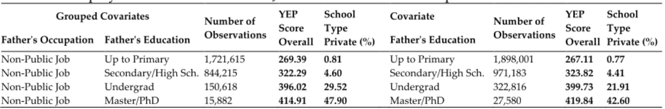
Interpretation style described above is similarly appropriate for mother’s education, father’s occupation, mother’s occupation and student’s own room at home. However in terms of father’s occupation, for the observant eye there lies one more caveat. We normally desire precisely categorized categorical variables in our analysis in which sense each category inhabits very similar, tightly defined properties that we can argue them as lying within an acceptable boundary and not overlapping with other categories. Except for father’s occupation, categorization of covariates considered in this study could be argued to possess from straightforwardly unequivocal (such as gender) to satisfactory categorization. For father’s occupation, there is no overlap between the other category subgroups which are non-working and public-worker as those can be strictly differentiated from non-public worker. However, within non-public worker sub-category there exist several subgroups which could be considered to possess considerably different characteristics. This subgroup involves a very wide

this sub-category. Moreover, the size of the sub-category for fathers with 2,765,215 individuals is quite large compared to mother for whom the number is 618,323. At the best case, we would desire to divide this sub-category to at least two sub-groups. That would be much more informative. Unfortunately, we do not have data at that resolution. However, as we can expect a correlation between job status and education level of father, we can explore if this could be informative about what is going on within non-public worker subcategory. In Table-5, left box show the summary of sub-classification done by grouping father’s occupation and father’s education covariates. The right box presents results for father’s education alone. What we observe is that father’s education seems to reflect enough the degradation within the subcategory as the distribution of results are quite close in both boxes. So controlling for father’s education at the same time with father’s occupation and/or adding an interaction term instituting both covariates seems to solve most of the problem.

Table 5. Interplay between of Non-Public Job Status of Father’s Occupation and Father’s Education Grouped Covariates _{Number of}

Observations YEP Score Overall School Type Private (%) Covariate _{Number of} Observations YEP Score Overall School Type Private (%) Father's Occupation Father's Education Father's Education

Non-Public Job Up to Primary 1,721,615 269.39 0.81 Up to Primary 1,898,001 267.11 0.77

Non-Public Job Secondary/High Sch. 844,215 322.29 4.60 Secondary/High Sch. 971,183 323.82 4.41

Non-Public Job Undergrad 150,618 396.02 29.52 Undergrad 322,816 399.73 21.91

Non-Public Job Master/PhD 15,882 414.91 47.90 Master/PhD 27,580 419.84 42.60

In terms of socio-economic development level of the city in which the student is living in, the average score of 6th level, i.e. the lowest development level, is 241.95 points, whereas the average scores

of other five levels are condensed within a narrow interval of 297.50 and 308.64 points. Moreover, there is no solid association between the level increments and average BAS score improvements. For example, while 5th _{level average is 297.50 points, it rises to 305.84 points for 4}th _{level, but falls back to 297.57 points}

for 3th level. In terms of the geographical region that the student lives in, Eastern Anatolia with 300.60 points and South-eastern Anatolia with 311.89 points are observed to differentiate from the remaining pile of regions whose average BAS scores are condensed within a narrow interval of 300.60 and 311.89 points. On the other hand, the group of cities whose development level is 6 are same as the cities of East Anatoli and South East Anatolia combined. In this context, outcome only varies considerably between this group of cities and remaining pile of cities. Hence, in order to improve the significance, precision, and degree of freedom of the analysis, it can be considered to form a new variable called City Development Index, which is equal to 1 for the group of least developed cities mentioned above, and is equal 0 for remaining cities.

In terms of resident type of the family, only students whose family lives in public quarters differentiate significantly in terms of BAS score and treatment assignment ratio. Moreover, the imbalance between treated and control groups are not as pronounced as the covariates mentioned above. So it’s less confounding and moreover because of less imbalance, confounding does not translate into a problem at the same scale. In terms of gender covariate, girls seem to achieve better BAS scores with around 5% higher in the treated group and 10% higher in the control group. However gender is not much a confounding covariate as the treated ratio is nearly same for both groups (4.73% vs 4.37%) while the two groups are nearly balanced: boys constitute 53.75 in the treated group and 51.71 in the control group, which are very close. For father’s life status, mother’s life status, and parents’ marital status, ratio of treated and BAS scores in treated and control groups vary as the status changes, albeit at a quite smaller size compared to strongly confounding variables mentioned above. However, because of relatively higher balance between treated and control groups, small overall confounding effect could