A Critical Review on Electromagnetic Precursors and
Earthquake Prediction
Levent SEVG˙I
Do˘gu¸s University, Electronics and Communication Engineering Department, Zeamet Sok. No. 21, Acıbadem / Kadık¨oy, 34722 ˙Istanbul-TURKEY
e-mail: [email protected]
Abstract
Seismo-electromagnetic precursory-based earthquake prediction studies are criticized in terms of their scientific content, problem complexity, signal excitation and propagation, causal relations with earth-quakes, and public awareness and expectations. One aim is to trigger a new debate on this hot topic in the Electromagnetic Society.
1.
Introduction
An earthquake is the sudden movement of the earth’s surface from the release of energy in the earth’s crust. The earthquake prediction (EP) is to assign a specific date, location, and magnitude for an earthquake within stated uncertainty bounds. The goal of the EP is to give warning of potentially damaging earthquakes early enough to allowappropriate response to the disaster, enabling people to minimize loss of life and property. The research on EP has a long history that went back to late nineteenth century and has attracted attention even in highly prestigious journals (see, e.g., [1-8] and references listed there). Obviously, prestigious journals like Nature, Science, IEEE Spectrum, etc., encourage publications as well as debates related to futuristic revolutionary studies, ideas, discoveries, which are believed to have to be a potential boon to humankind, and precursory-based EP is one of those topics. Although highly optimistic reports have been presented from time to time none has withstood detailed scientific examination and gradually falls to oblivion. The February 1999 Nature Debate [9] has many papers discussing the possible signals of different phenomena including seismicity, electricity, and luminosity that either accompany or are followed by earthquakes.
A detailed reviewpresented by Geller [1] criticized all these studies in terms of their scientific content and concluded that “The idea that there must be empirically identifiable precursors before earthquakes is
intuitively appealing, but studies over the last 120 years have failed to support it, therefore the occurrence of individual earthquakes is unpredictable”. The, more or less, overall attitude towards the issue of the
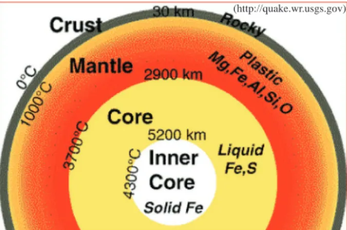
EP [10] is that “the earth is a complicated nonlinear system (see Figure 1); the crust can be activated
seismically with relatively small perturbation of the overall driving conditions; the complicated and non-linear seismology lacks a universally agreed physical model; the randomness in the initiation of a large rupture foils the use of short prediction windows; earthquake occurrence is effectively stochastic and consequently efforts at achieving deterministic prediction seem unwarranted; faults and fault systems are inhomogeneous; seismicity at almost all scales is absent from most faults before any large earthquake on that fault; earthquakes clearly
respond to stress changes from past earthquakes but the response is complex; very large earthquakes occur too infrequently to test hypotheses on how to predict them with the statistical rigor one would like; there is as yet no satisfactory theory about the nucleation of earthquakes; there is only a rudimentary understanding of the physics of earthquake ruptures; predicting earthquakes requires an understanding of the underlying physics, reliable earthquake precursors are not only difficult to determine, but they are, on precise physical grounds, unlikely to exist.”
(http://quake.wr.usgs.gov)
Figure 1. Earth’s crust, mantle and core (http://quake.wr.usgs.gov).
Although Geller’s study [1] is an excellent critical reviewit is obvious that EP debate continue to be a hot topic in the future. The aim here is not to repeat Geller’s critics; it is to discuss the scientific content of EP within the scope of electromagnetic precursors and causal relation, modeling of a sensor fusion problem, and, scientific responsibility and public awareness. Seismo-electromagnetic precursory-based EP studies have appeared in the scientific literature and media for many decades, but the motivation has come from recent publications of [10-11], therefore it is the right time and ELEKTRIK is the right journal to discuss all these issues. It should be noted that this paper is not about saying that ”EP is impossible”; it is solely about whether or not these studies are conducted scientifically. The problem is not to decide whether or not earthquake prediction is possible, it is to decide whether or not there are scientific and societal grounds at present for funding large-scale prediction research programs.
2.
Seismicity, Earthquakes and Prediction
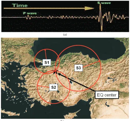
Seismic waves are the mechanical waves of energy caused by the sudden movement of the earth’s crust or an explosion that travels through the earth ([12-13] are excellent sources for all level of explanations with nice illustrations). In addition to surface waves, body waves of primary (P)-waves, and secondary (S)-waves are excited. The P-wave, move in a compressional motion longitudinally, is the fastest seismic wave that can move through solid rock and fluids, like water or the liquid layers of the earth. The S-wave, move in a shear motion perpendicular to the direction the propagating wave, is slower than the P-wave and can only move through solid rock. Their average speeds are about 6 km/s and 4 km/s, respectively. Although wave speeds vary by a factor of 10 or more in the earth, the ratio between the average speeds of a P- and S-waves is quite constant. This fact enables to simply record the time delay between the arrivals of the P- and S-waves to reasonably accurate estimation of the distance to the earthquake epicenter (see Figure 2a for a recorded real seismic signal example). The principal use of seismograph networks is to locate earthquakes. It is accurately possible to locate an earthquake occurred by using at least three stations. Roughly, multiplying
the time delay between S- and P-waves, in seconds, by the factor 8 km/s yields the approximate distance in kilometers. Drawing a circle on a map around the station’s location, with a radius equal to the distance, shows all possible locations for the event. The circle around the second station and intersections with the first one narrows the possible locations down to two points. Finally, the third station’s circle is used to identify which of the two previous possible points is the real one. This procedure is called triangularization (see Figure 2b).
(a)
(b)
Figure 2. (a) A seismograph record of 1989 Loma Prieta earthquake recorded 8400km away in Kongsberg, Norway showing the time delay between P- and S-waves, (b) A schematic illustration of earthquake epicenter location via triangularization. Seismograph stations are marked with “S”.
Although there are a fewothers, the Richter scale, named after Dr. Charles F. Richter of the California Institute of Technology, is the best known scale for measuring the magnitude of earthquakes. The scale is logarithmic so that a recording of 7, for example, indicates a disturbance with ground motion 10 times as large as a recording of 6. An earthquake of magnitude 2 is the smallest quake normally felt by people. Earthquakes with a Richter value of 6 or more are commonly considered major; great earthquakes have magnitude of 8 or more on the Richter scale. The amplitude of S-wave recorded with the seismographs is used to measure earthquake magnitudes.
As explained in Figure 2b, networks of different number of seismographs are used to measure the location and intensity of an earthquake after its occurrence. Although the time delay between P- and S-waves of the occurring earthquake can be used for early warning this may allow a response time in the orders of seconds depending on the distance of the earthquake epicenter (e.g., 10s-15s for an earthquake occurred approximately 100km away). These types of networks are used for fully-automatic shut-down of central gas and electricity systems to prevent large scale explosions and fire.
Early-warning-aimed EP methods, in general, could be divided into two; statistical methods for seismicity and observation of precursors to large earthquakes. Long-term projections of an earthquake
in a certain area with a high probability within some decades is possible by studying historical earthquake records, monitoring the motion of the earth’s crust by satellite, and measuring with strain monitors below the surface. This is important for the policy makers. But, short term EP require to state precisely where (hypocenter latitude and longitude), when, at what depth, how strong, and with what probability the earthquake occurs within the stated error/uncertainty bounds.
EP methods, by far, are away from their mature stage and are controversial. Methods/models based on physical and geological data (observations and experimentations) are totally different from statistical methods/models using either past (retrospective) or future (prospective) average rate of earthquake occur-rence within pre-specified limits of hypo-central latitude, longitude, magnitude, depth, and time (none of which can be estimated without uncertainty). Even statistical models have fundamental differences on their assumptions, approximations, and approaches. Some are grid-based, while others may be fault-based, some use quasi-stationary assumption (i.e., earthquake rates are assumed relatively stable over a year or more), while the others assume short-term (day-by-day, or weekly) variations, etc. [8].
Experts who use statistical models prefer to name their study as “earthquake forecast ” and refer “earthquake prediction” to a single earthquake as a special case of a forecast with temporarily and excep-tionally high probability and imminence. More importantly, they consider their studies and statistical test results as a tiny step towards physical understanding of earthquakes and occurrence.
Table 1 list a year-average of the number of different-magnitude earthquakes; there are approximately 80,000 per month and 2,600 per day. Apparently, it is statistically possible to make strong guesses on where and when earthquake hits next time. The only thing you should do is to make a guess, wait for a while, and then arbitrarily correlate any of the frequently occurring nearby earthquakes with your guesswork. It doesn’t matter that it is an unscientific prediction, since scientists can not state that the predicted earthquake will not occur, because an event could possible occur by chance on the predicted intervals.
Table 1. Average yearly earthquake occurrence.
Description Magnitude Occurrence/year
Great 8.0+ 1
Major 7.0-7.9 18
Large (destructive) 6.0-6.9 120
Moderate (damaging) 5.0-5.9 1,000
Minor (damage slight) 4.0-4.0 6,000
Generally felt 3.0-3.9 49,000
Potentially perceptible 2.0-2.9 300,000
Imperceptible less than 2.0 600,000+
The International Association of Seismology and Physics of the Earth’s Interior (IASPEI) outlined guidelines for precursory-based EP [1,5]. According to these guidelines observed anomaly should have a relation to stress, strain, or some mechanism, leading to earthquakes, should be simultaneously observed on more than one instrument, or at more than one site, and should bear an amplitude-distance correlation. There should be a persuasive demonstration that the calibration of the instrument is known, and that the instrument is measuring a tectonic signal. Anomaly definitions should be precisely stated so that any other suitable data can be evaluated for such an anomaly. The difference between anomalous and normal values shall be expressed quantitatively, with an explicit discussion of noise sources and signal-to-noise ratio. The rules and reasons for associating a given anomaly with a given earthquake shall be stated precisely. The probability of the “predicted” earthquake to occur by chance and to match up with the precursory anomaly
shall be evaluated. The frequency of false alarms (similar anomalies not followed by an earthquake) and surprises (similar size mainshocks not preceded by an anomaly) should also be discussed.
No earthquake prediction methods based on precursors satisfying these guidelines have ever been observed for the period of more than a century [1].
3.
A Multi-sensor Fusion (MSF) Problem
What has been suggested in most of the seismo-electromagnetic precursory-based EP is nothing but a multi-sensor fusion system. I believe it would be better to review an example of MSF system with quite similar complex signal environment before discussing seismo-electromagnetic precursory-based EP. For example, an integrated maritime surveillance (IMS) system discussed in [14-15] uses all possible information to picture surface and air activities over coastal areas. The Vessel Traffic Management System of Turkish Straits [16] may be given as another sensor fusion example. I have involved in these types of systems for more than a decade and I have still been experiencing difficulties with the complexities of these problems.
Radar is a device that transmits and receives electromagnetic waves to detect the presence of targets and to extract as much information as possible from interaction of electromagnetic waves with objects. A radar target is the object of interest that is embedded in noise and clutter together with interfering signals. Location of a target with a radar system requires determination of its range (radial distance), azimuth (angular position) and height intervals. Noise is a floor signal which limits the smallest change that can be measured in the receiver. Clutter is a radar (background) echo or group of echoes from ground, sea, rain, birds, chaff, etc., that is operationally unwanted in the situation being considered. There is no single definition for clutter, and clutter/target may interchange depending on the duty of the radar. For example, an echo from rain is clutter for an air surveillance radar, but is the target for a whether radar. Similarly, ground echo is clutter for ground surveillance radar, but is itself the target (useful signal) for a ground imaging radar.
A total radar echo usually consists of target, noise, clutter, and interference signals, all of which randomly fluctuate with time. This means, a radar signal environment is a stochastic environment. Usually, the target signal is embedded within a background (noise + clutter + interference), its power level is much less than the others and it is extremely difficult to extract it. The process of extracting useful information (generally the target) from the total echo is called (stochastic) signal processing and performed via powerful, intelligent algorithms. The power of these algorithms arises from the physical understanding of the target, noise, clutter and interference signals.
Target detection is the ability to distinguish target at the receiver. Target tracking is the process
of following the moving target continuously, i.e., to monitor its range, direction, velocity, etc., and mainly deals with the correlation of current detections with previous ones. Target classification is to distinguish certain types of targets and group them according to certain characteristics called “features”. Possible distinguishing features may be their size, speed, on-board electronic devices, electromagnetic reflectivity, maneuvers, etc. Target identification is the process of finding out “who” the target is. This knowledge of a particular radar return signal that is from a specific target may be obtained by determining size, shape, timing, position, maneuvers, rate of change of any of these parameters, by means of coded responses through secondary radar, or by electronic counter measures. Integrated surveillance is the systematic observation of a region (aerospace, surface or subsurface areas) by a number of different sensors, primarily for the purpose of detecting, tracking, classifying and identifying activities of interest.
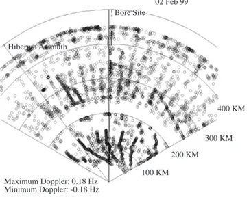
An integrated maritime surveillance system was designed for the east coast of Canada based on two, high frequency surface wave (HFSW) radars [14-15]. HFSWR are coherent radars and detection is based on the signal-to-noise ratio in the frequency (Doppler) domain with an extremely high false alarm rate (FAR). An example is presented in Figure 3. Here, total detections recorded within hour period for one of the SWHFR in Feb. 2, 1999 have been plotted on a range-azimuth scale with tens of thousands of false alarms (detections) dominated by ionospheric and ocean clutter. The 10 to 20 surface target tracks among the large number of false detections may be observed in the figure.
Bore Site Hibernia Azimuth 02 Feb 99 400 KM 300 KM 200 KM 100 KM Maximum Doppler: 0.18 Hz Minimum Doppler: -0.18 Hz Cape Race
Figure 3. Total detections in 60-min record time for Cape Race HFSWR recorded in Feb 2, 1999 showing the high false alarm rate.
So, the question is: Howcould we obtain an acceptable performance with this IMS system? The answer resides on the understanding of details of electromagnetic signal environment. An example of three dimensional contour plot of one of the IMS radar data as signal strength vs. Range-Doppler bins along one azimuth (beam) direction at 3.4 MHz for a wind speed of 40-50 knot is plotted in Figure 4. The colors (grayscale) correspond to the signal strength, the darker the point the higher the signal strength. Remember, a target at any range with any speed (i.e., Doppler frequency) is just a dot on this plot. This is the signal environment where the radar detector automatically specifies the threshold and gives the “detected” decision. Two vertical cuts of such a figure recorded in Sep 19, 1999 after the elimination of environmental noise are presented in Figures 5 and 6 [14-15]. In Figure 5, range profile at 11:00am for almost stationary targets
(i.e., at 0 Hz) along one azimuth direction (87.1◦) is given. The peaks at ranges between 300 km-400 km
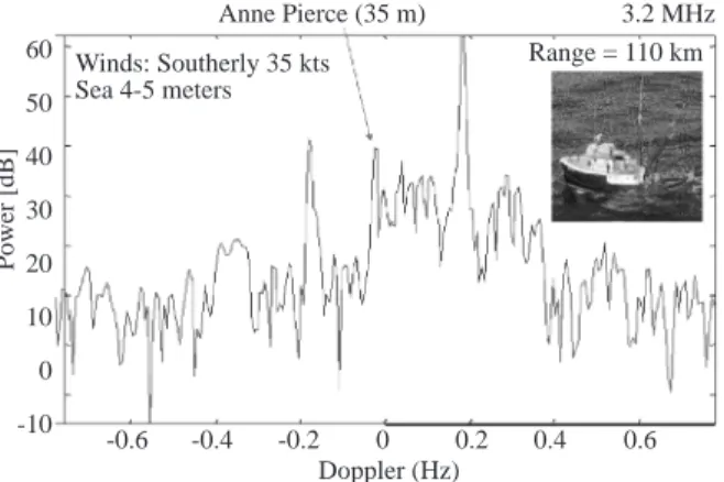
are the echoes from three Canadian off-shore oil platforms, and the other two peaks at ranges 100km and 200km belong to E and F layer-reflected clutter. The plot in Figure 6, which was recorded just an hour later showed only two of the oil platforms and obviously ionospheres clutter disappeared. Finally, an example of a horizontal cut of Figure 4 is given in Figure 7, showing the Doppler power spectrum of a range bin at 110
km away from the shore at 3.2 MHz operating frequency, with the two dominant Bragg peaks at ±0.2 Hz
representing echoes from the ocean waves that resonate with the radar signal, and the 35m-long boat Ann Pierce at approximately -0.03 Hz.
Range
-V 0 V
Figure 4. A three dimensional contour plot of Cape Bonavista HFSWR data as signal strength vs. Range-Doppler bins (Beam 26, 120.4◦, f=3.4 MHz) for a wind speed of 40-50 knot.
80 70 60 50 40 30 20 10 0 Power [dB] E Layer F Layer Hib Glomar Bills 100 150 200 250 300 350 400 450 Range [km]
File: sbpf-cr-sep9-1100.dat, All Ranges, Doppler 52 (0 Hz), Beam 6 (85.8 deg), Freq 3.2 MHz
Figure 5. A range profile at 0 Hz along one azimuth direction (87.1◦). The peaks atranges between 300 km-400 km are the echoes from three off-shore oil platforms (vertical axis is dB above the thermal noise, Sep 9, 1999 data at 11:00am). Hib, Glomar, and Bills are the off-shore oil platforms in Canadian East Coast at approximately 300km-350km. 80 70 60 50 40 30 20 10 0 Power [dB] Hib Bills 100 150 200 250 300 350 400 450 Range [km]
File: sbf7-cr-sep9-1140.dat, All Ranges, Doppler 54 (0 Hz), Beam 7 (87.1 deg), Freq 3.3 MHz
Figure 6. A range profile at 0 Hz along one azimuth direction (87.1◦). The peaks atranges between 300km-400 km are the echoes from three off-shore oil platforms (vertical axis is dB above the thermal noise, Sep 9, 1999 data at 12:00am, showing E and F layer reflections).
60 50 40 30 20 10 0 -10 Power [dB] 3.2 MHz -0.6 -0.4 -0.2 0 0.2 0.4 0.6 Doppler (Hz) Anne Pierce (35 m) Range = 110 km Winds: Southerly 35 kts Sea 4-5 meters
Figure 7. A Doppler power spectrum of a range bin at 110km away from the shore at 3.2MHz operating frequency, showing the Bragg peaks and the 35m-long boat.
Don’t you think it is a real challenge to suppress strong Bragg peaks, E- and F-layer clutter and discriminate much weaker target echo? Yes, indeed it is a challenge! Ionosphere is a time-varying non-homogeneous media where the electron content (virtual electromagnetic layers) varies with height, latitude and longitude, and showdaily, seasonal, yearly variations. Only after recordings of a fewdecades (many sun-cycles of 11 years) one can get a very rough idea of average characteristics of the ionosphere in a region. Same is true for the ocean wave – electromagnetic wave interaction and the environmental noise. We are still far away modeling ocean clutter, especially at high sea states (i.e., for high ocean waves developed after strong storms). Target reflectivity is another challenge to deal with.
Fortunately, these systems are based on active sensors, which means the radar produce its own signal and have a complete authority on the specification of signal characteristics such as frequency, power, duration, modulation, encryption, etc. Moreover, sensors transmit signal continuously and receives (millions of) echoes which makes it possible to apply all kinds of digital signal processing techniques such as coherent/non-coherent integration, filtering, correlation, etc. It is only after these processes that target signal could be discriminated from all other unwanted echoes in extremely complex electromagnetic environment and under very high false alarm rate conditions.
Scientific prediction is possible if and only if a “precise” model of a real-world problem could be established. A model is defined as a physical or mathematical abstraction of a real world process, device or concept. Building a model means doing simplifications, approximations, assumptions, neglecting many parameters, and finally moving onto an artificial environment if discretized in computers. Therefore, one should be extremely careful when dealing with models. For example, take a radar cross-section (RCS) prediction problem and look at the airplane and its discrete computer model in Figure 8. Can you imagine, accept and feel comfortable when one does computer predictions using the discrete model given in this figure instead of the real airplane? Yes, we can use even this over-simplified model, if we can’t build or don’t have better ones, up to certain extend, and in order to just get the feeling of the RCS behavior, not for the accurate calculations and predictions.
Think about cellular phone – human tissue interaction problem; the specific absorption rate (SAR) modeling studies where experts use either discrete computer models or phantoms of different jells and chemical substances, both of which are electromagnetic “equivalents” of the human head. Although they are based on extensive amount of precise permittivity and conductivity values supplied by the measurement
the head and kept in a jar can not be the same brain of a living person. Therefore, is it reliable to conclude that the results would have been the same if it would have been possible to measure SAR directly inside an alive human head? Of course, not! Scientists are well-aware of the simplicity of the SAR models used and do not jump generalized conclusions from the results of SAR measurements.
Real world (complex)
Discrete model (simple)
Figure 8. A photograph of an airplane and its over-simplified discrete computer model used for RCS predictions.
4.
Electromagnetic Precursory-based Earthquake Prediction
The necessary and sufficient conditions of a precursory-based EP are to observe and discriminate the
quantity, to show the causal correlation, and finally, to build a model . Now, imagine the signal environment
for seismo-electromagnetic precursory-based EP system, where one must consider not only earth’s surface and atmospheric environment, but also the whole electro-mechanical environment under the earth’s surface (underground electromagnetic scattering is even more complex so experts who deal with the recognition of buried objects prefer to name their study as “subsurface imaging” instead of “mine-detection”).
There may be variety of earthquake precursors from acoustic, electromagnetic signals to infrared emissions on the ground as well as in the ionosphere in a broad frequency range from mHz up to MHz [17-23]. One can observe variety of physical quantities, such as ionosphere electron content, environmental noise, surface and subsurface irregularities, ground conductivity, earth’s magnetic field, electric field, ocean surface currents, satellite imagery, infrared (thermal) camera, etc. On the other hand, any phenomena that happened to occur before an earthquake can be called precursors whether or not they have a causal relation to the earthquake, therefore, observations of these signals and studies for their correlation with the earthquakes are only worthwhile if issued scientifically. Efforts towards the data gathering of earthquakes occurring with and without preceded precursors are extremely important. But, as presented in [10], jumping directly a conclusion from these very early stage studies that accurate earthquake early warning is within reach within a decade is not scientific.
VAN method is one of a fewof seismo-electromagnetic precursory-based EP studies. The VAN group claim that seismo-electric (SES) transient signals are electromagnetic precursors triggered by the imminent earthquakes, so these can be observed for EP purposes [24-26]. It is a quasi-static ground conductivity measurement system with horizontally and vertically buried electrodes. They claim that SES exist, only if one chooses right spots (sensitive stations), and only less than %0.1 of observed changes are meaningful signals, all others being noise. VAN group and followers have admitted that physics of the SES has not been completely clarified yet (see [1] for Geller’s critical review)!
Another group [27] claim that there is a transient change of static electrical field of the earth, appear sometime before earthquake, caused by the regional, stress and strain. Their high-sensitive (!) monopolar probe system (MPS) measures transient electric fields which are claimed to be related to the earthquake
based electromechanical changes. A forecast, a network of multi-MPS, system has been established (see http://www.deprem.cs.itu.edu.tr) to be used in EP, based on the recorded transient electrostatic displace-ment close to the Earth’s surface, sometimes just a fewminutes, sometimes day, even months before the earth-quake occurs (read a comment and a reviewer evaluation for a paper of this group in the next ELEKTR˙IK issue; and see how low-quality and pseudo-scientific works can possibly be published in scientific journals).
Another group claimed that a network of passive sensors (magnetometers) can be used in EP by using the transient change in earth’s magnetic field prior to imminent earthquakes, and this was recently published in the IEEE Spectrum [28]. I am concerned about the way in which this topic was presented in terms of public awareness, interest, and expectations [29-30]. The authors claim to predict California earthquakes sometime before, if the region is covered by a network of 200-300 ground-based magnetometers. They said, ground-based sensors can be used to monitor changes in the low-frequency magnetic field as well as to measure changes in the conductivity of air at the earth’s surface. Moreover, they said they can monitor noise levels at extremely lowfrequency (ELF)—below300 Hz by using satellites, observe the earthquake-related infrared light, even use existing GPS system to detect changes in the total electron content of the ionosphere that occur days, even weeks before the earthquakes.
One thing is common among all these three studies; electric and magnetic fields ranging from mHz up to a fewMHz are seismo-electromagnetic precursors of earthquakes and can be used in EP. Electromagnetic engineers who deal with low frequency signals are aware of complexity in these frequency ranges, since environmental noise and electromagnetic wave propagation possesses almost global characteristic, highly sensitive to fine details of fluctuations in a large volume, not just in the immediate vicinity of earthquakes, and localization by any means is hardly possible. For example, atmospheric noise in a region depends on daily lightning (cloud-to-ground discharges) and flashes (cloud-to-cloud discharges) along the equilateral region; a strike, for example in North Africa, causes atmospheric noise fluctuations in Europe and USA. Similarly, lightening and flashes cause a fewHz vertically and horizontally polarized waves, respectively, which travel all around the earth through earth-ionosphere waveguides (Schumann resonances). It is extremely difficult, if not impossible, to distinguish local seismo-electromagnetic signals from these global effects even if the latter have been monitored for many decades.
Even though I have nearly two decades of experience on electromagnetics, wave scattering, radiowave propagation through complex environments, radar systems design, signal processing aspects including de-tection, tracking, classification and identification I am quite frightened by the courage of those people who claim to measure/record earth’s seismo-electromagnetic signals with their highly sensitive (!) devices, truly astonished by the hypotheses they introduce and oversimplified assumptions they use in explaining extremely complex phenomena, without focusing on the ducting, anti-ducting, guiding-to-anti-guiding transitional ef-fects of seismo-electromagnetic waves both under and above the earth’s surface through inhomogeneous propagation media characterized by local permittivities, permeabilities and conductivities with all electro-acousto-mechanical interactions.
Understanding characteristics of the noise- and clutter-like signals before dealing with signal discrimi-nation is a must. Just to give an idea, time variations of two signals are plotted in Figures 9 and 10. Can you identify these signals if I give you a list of possible sources? Do they belong to the measurement of a 24-hour variation of atmospheric noise that has been recorded in the UK for nearly 30 years, or a 6-hour electrostatic record of the precursory patterns due to structural changes in Istanbul, a 4-day electron content variation of the F1 layer of the ionosphere recorded in Izmiran Space Research Center in Russia, a boundary-layer-refractivity variations in Istanbul in recorded Feb 2000, a 24-hour earth’s magnetic field variation displayed
with the York Station of SAMNET project in the UK (www.dcs.lancs.ac.uk/iono/samnet), or a 20-min TV intermediate thermal noise recorded at Sony? Can they be a time variation of a computer generated cell phone received signal through a numerically modeled fading channel? Or, are they the plots of daily variation of Top-100 stocks in Istanbul Stock Exchange? Do you think they are measured, or recorded, or synthetically produced via a few-line Matlab scripts which use random number generators?
?
time Figure 9. Time variation of a noise (clutter)-like signal.
?
time Figure 10. Time variation of another noise (clutter)-like signal.
All could be done currently in these seismo-electromagnetic signal-based EP studies is to try to showthat the recorded anomalies within all other anomalies are related to the earthquakes occurred,
sometimes a fewhours, sometimes several days (even months) afterwards, only after the earthquakes
occur (retrospective correlation!). What’s missing currently in these studies is the falsification principle of Karl Popper; i.e., the systematic rule out of the known natural and artificial sources of signals from the precursors of the earthquakes. Those who continuously record ionosphere noise, electron content, virtual layer heights, magnetic field changes of the Earth’s surface, static and/or quasi-static electric / magnetic fields, electromagnetic and infrared radiations, etc., and perform EP have this unique hypothesis: “there
is some relation between the anomaly observed and earthquakes but the mechanism and parameters of this relation are yet unknown”.
5.
Conclusions and Discussion
Scientific study is distinguished from “pseudo-science” or from “metaphysics” by its empirical method, proceeding from observations, experiments and calculations. One can not respond a question of “why” by just saying “because I said so!” He/she should postulate and well-define the problem (state approximations, assumptions, simplifications), discuss and showexistence, uniqueness, and convergence of the solution, present the accuracy, resolution, precision, state error/uncertainty bounds, and finally, build a model so that anybody who follows the same procedure is able to reach the same result.
Well-accepted universal criteria for the scientific process are the objectivity (running always after the
truth), systematicity (establishing the causal correlation), reliability (obtaining similar results with similar methods), repeatability (different people should reach similar results), comprehensiveness (stating the bounds of uncertainty), and the predictive power.
Here, the precision and the predictive power are the keywords. The real world is extremely complex and no model is precise, and no model can predict accurately, when dealing with natural phenomena. The degree of precision and predictive power achieved is only a question of building reliable models. The fact that geophysicists have not developed their models that are as precise and predictive as, for example, communication or microwave engineers, does not necessarily mean that Earth science is less scientific, but merely refers to the requirement of the development of “better” or “more realistic” models.
The Nobel laureate chemist, I. Langmuir summarized “pathological science” as follows [1,32]:
• The maximum effect that is observed is produced by a causative agent of barely discernible intensity,
and the magnitude of the effect is substantially independent of the intensity of the cause.
• The effect is of a magnitude that remains close to the limit of detectability (high sensitivity), or many
measurements are necessary because of the very lowstatistical significance of the results.
• There are claims of great accuracy.
• Fantastic theories contrary to experience are suggested.
• Criticisms are met by ad hoc excuses thought up on the spur of the moment.
• The ratio of supporters to critics rises up to somewhere near % 50 and then gradually falls to oblivion.
The artificial optimistic impression pumped recently via these seismo-electromagnetic precursory-based pseudo-scientific EP studies is seriously concerning. Giving a wrong impression that we’ll be able to work out all the prediction problems and soon build systems which warn people hours, even days before strong earthquakes (as presented in [10]) is extremely dangerous in countries with poor scientific literacy where municipalities fearlessly extend city plans right through the faults; people construct weak buildings, etc. It should be noted that it is not earthquakes themselves which kill people; it is the collapse of man-made
structures which does most of the damage, therefore the best way of preparing the society for strong and devastating earthquakes and to mitigate their worst effects is to develop better urban land use plans and construct stronger buildings. If, highly artificial optimism is imposed via these highly respectful journals
that earthquake early warning systems will be ready in a few years people, rather than taking measures to improve building safety, will prefer to rely on “experts” to predict the time of an earthquake to protect themselves.
The claim, no matter howdifficult the problem may be, the research must continue, is based on an (unrelated) analogy established between earthquake prediction research and others, such as cancer research, weather forecast, etc. If the aim is to minimize fatality and damage due to earthquakes, the solution is the application of hazard mitigation techniques, not issuing inaccurate and unreliable earthquake alarms. The design of earthquake-resistant buildings should be the priori job. Vague earthquake predictions would be harmful, not helpful, to society.
One defensive argument those electromagnetic precursory-based EP people and their fans and fol-lowers, even some of my students is that how humanity would have progressed in science and technology without imagination (thinking big) of, for example, going to stars, building escalators to moon, etc. As I
indicated in [28], imagination is definitely one of the triggers, but not the only one. The philosophy should be “Think big but stick with the scientific methods and proceed step by step”.
In conclusion, the scientific goal should be the understanding of fundamental physics of earthquakes and physics-based theory of the precursors (their causal correlation), not the reliable prediction of individual earthquakes. In viewof the lack of proven forecasting/prediction methods, everybody should exercise caution in issuing public earthquake warnings. The efforts should be focused on the elimination from scientific journals of scientifically low-quality works, the exposure of works that contains errors and absurd statements made by scientifically unqualified publicity seekers.
Don’t you agree that the scientific society should expect and deserve more than what Gary presents (see Figure 11)?
Figure 11. Gary’s forecasts including earthquakes (http://www.partyfolio.com).
References
[1] R. J. Geller, “Earthquake prediction: A critical review”, Geophys. J. Int., Vol. 131, pp. 425-450, 1997.
[2] Y. Y. Kagan, L. Knopoff, “Statistical short-term earthquake prediction”, Science, Vol. 236, pp.1563-1567, 1987.
[3] R. B. Schall, “An Evaluation of the Animal-behavior theory for earthquake Prediction”, California Geology, Vol. 41, No. 2, pp. 41-45, 1988.
[4] R. J. Geller, “Shake-up for Earthquake Prediction”, Nature, Vol. 352, pp. 275-276 (also Vol. 353, pp.612), 1991.
[5] M. Wyass (Ed.), Evaluation of Proposed Earthquake Precursors, Am. Geophys. Un., Washington, 1991.
[6] P. Varotros, O. Kulhanek, (Eds.), “Measurements and Theoretical models of the Earth’s Electric field Variations Related to Earthquakes”, Special issue, Tectonophysics, Vol. 224, pp. 1-288, 1993.
[7] McGuire et al, “Time-domain observations of a slow precursor to the 1994 Romanche transform earthquake”, Science Vol. 274, pp.82-85, 1996.
[8] R. J. Geller, D. D. Jackson, Y. Y. Kagan, F. Mulargia, “Earthquakes cannot be predicted”, Science, Vol. 275, pp.1616-1617, 1997.
[9] Nature Debate on Earthquake Prediction, www.nature.com/nature/debates/earthquake, on the internet, Feb 1999.
[10] Tom Bleier, Friedemann Freund , “Earthquake Alarm”, IEEE Spectrum, Vol. 42, No.12, pp. 16-21 (int), Dec 2005.
[11] http://www.earthquakeprediction.gr/index.htm.
[12] http://quake.wr.usgs.gov/info/eqlocation/index.html for an earthquake location tutorial.
[13] http://quake.wr.usgs.gov/research/seismology/index.html.
[14] L. Sevgi, A. M. Ponsford, H.C. Chan, “An Integrated Maritime Surveillance System Based on Surface Wave HF Radars, Part I – Theoretical Background and Numerical Simulations”, IEEE Antennas and Propagation Magazine, Vol. 43, No.4, pp.28-43, Aug. 2001.
[15] A. M. Ponsford, L. Sevgi, H.C. Chan, “An Integrated Maritime Surveillance System Based on Surface Wave HF Radars, Part II – Operational Status and System Performance”, IEEE Antennas and Propagation Magazine, Vol. 43, No. 5, pp.52-63, Oct. 2001.
[16] A. N. Ince, E. Topuz, E. Panayirci, C. Isik, Principles of Integrated Maritime Surveillance Systems, Boston, Kluwer Academic, 2000.
[17] A. V. Guglielmi, “Magnetoelastic waves”, Izvestiya AN SSR (Earth Physics), N7, 112, 1986.
[18] Pride-SR Haartsen-MW, “Electroseismic Wave Properties”, J. of Acoust. Soc. America, JASA-100, No. 3, pp 1301-1315, 1996.
[19] I. Yamada, K. Masuda, H. Mizutani, “Electromagnetic and acoustic emission associated with rock fracture”, Phys. Earth Planet. Inter., 57, 157-168, 1989.
[20] V. A. Liperovski, C. V. Meist er, E. V. Liperovskaya, N. E. Vasileva, O. Alimov, “On Spread – Es effects in the ionosphere before earthquakes”, Natural Hazards and Earth system Sciences, pp.59-62, 2005.
[21] A. Kotsarenko, O. Molchanov, M. Hayakawa, S. Koshevaya, V. Grimalski, R. P. Enriquez, J. A. Lopez, “Investigation of ULF magnetic anomaly during Izu earthquake swarm and Miyakejima volcano eruption at summer 2000, Japan”, Natural Hazards and Earth system Sciences, pp.63-69, 2005.
[22] K. Eftaxias, P. Kapiris, J. Polygiannakis, A. Peratzakis, J. Kopanas, G. Antonopoulos, D. Rigas, “Experience of short term earthquake precursors with VLF – VHF electromagnetic emissions”, Natural Hazards and Earth system Sciences, pp.217-228, 2003.
[23] R. Ludvin, www.geophys.washington.edu/SEIS/PNSN/INFO GENERAL/eq prediction.html
[24] P. Varotsos, K. Alexopoulos and K. Nomicos, “Seismic electric currents”, Practica, Athens Academy, 56, 277, 1981.
[25] P. Varotsos, K. Alexopoulos and K. Nomicos, “A method for the prediction of earthquakes” 4th Int. Conference on BasementTectonics, Oslo, 1981.
[26] P. Varotsos, K. Alexopoulos, K. Nominos, M. Lazaridou, “Earthquake prediction and electric signals”, Nature, 322, 120, 1986.
[27] B. ¨Ust¨unda˘g., O. Kalenderli, H. Eyido˘gan “Multilayer Capacitor Model of the Earth’s Upper Crust“ ELEK-TRIK, Turkish J. of Electronical Engineering and Computer Sciences, Vol. 13, No.1, pp. 163-174, 2005. [28] Tom Bleier and Friedemann Freund, “Earthquake Alarm” IEEE Spectrum, Vol. 42, No.12 (INT), pp. 17-21, Dec
2005.
[29] L. Sevgi, “Earthquake Early Warnings: Prediction or Guesswork”, IEEE R8 Newsletter, Vol. 9, No.1, pp. 11, Mar 2006 (www.ieee.org/r8).
[30] L. Sevgi, “Earthquake Early Warning: Prediction vs. Guess”, Comment to the “Earthquake Alarm” by Tom Bleier and Friedemann Freund, IEEE Spectrum Online, Vol. 42, No.12 (INT), pp. 17-21, Dec. 2005 (www.spectrum.ieee.org.csulib.ctstateu.edu/dec05/comments/1181).
[31] L. Sevgi, “On the Science, Scientific Process and Scientific Filter . . . ”, (Letter to the Editor), IEEE Antennas and Propagation Magazine, Vol. 44, No.2, pp.122, 2002