http://journals.tubitak.gov.tr/botany/ © TÜBİTAK
doi:10.3906/bot-1210-21
Classification of Camellia species from 3 sections using leaf anatomical data
with back-propagation neural networks and support vector machines
Wu JIANG1,2, Billur BARSHAN ÖZAKTAŞ3, Nitin MANTRI4, Zhengming TAO2, Hongfei LU1,*
1College of Life Science, Zhejiang Sci-Tech University, Hangzhou, P.R. China 2Economic Crops Laboratory, Institute of Zhejiang Subtropical Crops, Wenzhou, P.R. China 3Department of Electrical and Electronics Engineering, Bilkent University, Bilkent, Ankara, Turkey 4School of Applied Sciences, Health Innovations Research Institute, RMIT University, Melbourne, Victoria, Australia
1. Introduction
Genus Camellia L. (Theaceae), the large type genus of Theaceae family, is widely distributed in eastern and southeastern Asia (Shen et al., 2008; Jiang et al., 2012). However, the interspecies relationship of this economically important genus is still a controversy (Vijayan et al., 2009). While reliable classification of plants is of crucial importance in taxonomy, some principles of plant taxonomy such as morphological features, phylogenetic considerations and chemical and numerical taxonomy have been validly applied in Camellia taxonomic treatments (Lin et al., 2008; Lu et al., 2008a, 2008b, 2009; Pi et al., 2009; Jiang et al., 2010; Pi et al., 2011). To solve the discrepancies of Camellia taxonomy, the use of leaf characteristics was proposed (Ming, 2000; Kong, 2001). In particular, Lin et al. (2008) and Pi et al. (2009) suggested that leaf characteristics provide an effective foundation for further research of the genus Camellia.
Leaf characters like anatomical analysis have been successfully applied in plant research (Kumar et al., 2012; Vasic and Dubak, 2012). In addition, leaf characteristics
can be used in conjunction with supervised pattern recognition (SPR) techniques for taxonomic classification. SPR refers to techniques in which a priori knowledge about the category membership of samples is used (Roggo et al., 2003; Chen et al., 2009). The classification model is constructed by training sets with known categories and model performance is assessed by comparing sample categories predicted with true categories that form a prediction set (Roggo et al., 2003). As a mathematical tool for prediction of nonlinearities, artificial neural networks (ANNs) attempt to mimic the functioning of the human brain and are increasingly utilized in many fields owing to their excellent pattern recognition capability (Bila et al., 1999; Li and Yang, 2008; Zheng et al., 2011). Among all the ANNs, back-propagation artificial neural network (BP-ANN) is the most widely used (Mitchell, 1997). BP-ANN is trained by repeatedly presenting a sequence of input and output patterns to the network. The network gradually learns the relationship between the input and the output by adjusting the weights to minimize the mean-squared error (MSE) between the actual and predicted output patterns Abstract: Leaf characteristics provide many useful clues for taxonomy. We used a back-propagation artificial neural network
(BP-ANN) and C-support vector machines (C-SVMs) to classify 47 species from 3 sections of genus Camellia (16 from sect. Chrysanthae, 16 from sect. Tuberculata, and 15 from sect. Paracamellia). The classification model was constructed based on 7 leaf anatomy attributes including, area of adaxial epidermal cell, thickness of adaxial epidermal cell, thickness of palisade parenchyma, thickness of total leaf, thickness of spongy parenchyma, thickness of abaxial epidermal cell, and area of abaxial epidermal cell. Model parameters of C-SVM, comprising regularization parameter (C) and kernel parameter (γ), were optimized by cross-validation. The best classification accuracy of the 3 Camellia sections was achieved by the radial basis function SVM classifier (with parameters C = 32, γ = 0.13), as well as the sigmoid SVM classifier (with parameters C = 32, γ = 0.13), which was up to 84.00% in the training set and 90.91% in the prediction set, respectively. Compared with BP-ANN, SVM yields slightly higher prediction accuracy, which indicates that it is feasible to accurately classify the 3 sections of Camellia using SVMs based on leaf anatomy data.
Key words: BP-ANN, Camellia, leaf anatomy, plant numerical taxonomy, supervised pattern recognition, SVM
Received: 10.10.2012 Accepted: 07.06.2013 Published Online: 30.10.2013 Printed: 25.11.2013 Research Article
of the training set (Sadeghi, 2000). The network training is considered complete when the MSE of the test set reaches a minimum. The BP-ANN has been successfully utilized as a modeling tool in food technology, chemistry science, sensory analysis, bacteria predictions, beam identification, operations management, etc. (Giacomini et al., 2000; Guyer and Yang, 2000; Luo et al., 2004; Lu et al., 2010).
Support vector machines (SVMs) is another classification technique developed by the machine learning community (Vapnik, 1989; Cortes and Vapnik, 1995; Vapnik, 1995; Zheng et al., 2010). This technique fixes the classification decision function based on structural risk minimum mistake instead of the minimum misclassification error on the training set in order to avoid the problem of over-fitting (Chen et al., 2007). Moreover, SVMs are capable of learning in high-dimensional feature spaces and do not require large amounts of training samples (Burges, 1998). As a new pattern recognition tool, SVMs have been successfully applied in many areas such as fruit classification, text categorization, fault diagnostics, and object recognition (Pontil and Verri, 1998; Yuan and Chu, 2007; Turhan and Serdar, 2013). However, few studies about plant species classification using ANN or SVM have been reported. Very little information is available, especially on the classification of the genus Camellia based on ANN or SVM.
This study was undertaken to evaluate the feasibility of classifying species from 3 sections of Camellia using supervised pattern recognition techniques, BP-ANN, and SVM. This would provide a new approach for addressing the inconsistencies in Camellia classification.
2. Materials and methods 2.1. Plant materials
The plant materials were collected from the International
Camellia Species Garden in the city of Jinhua, Zhejiang
Province, China. Leaf samples for anatomical analyses were taken from the third mature leaf of old branches that were fully exposed to sunlight, from at least 3 plants per species. Healthy leaf samples (Table 1) consisting of 16 species from section Chrysanthae Chang, 16 species from section Tuberculata Chang, and 15 species from section Paracamelli Chang were examined in the present study following Chang’s classification (Chang, 1998). The specimens are deposited in the Chemistry and Life Science College of Zhejiang Normal University.
2.2. Anatomical protocol and data collection 2.2.1. Epidermal preparations
Approximately 1 cm2 of tissue was removed from the
middle area of the leaf and cut horizontally between the adaxial and abaxial surfaces into 2 halves. Next, 40% sodium hypochlorite solution was added to fully cover
the material for 10 min at 37 °C. Materials were stained in safranin-alcian green and mounted in neutral balsam after the mesophyll tissues were removed and the leaf epidermis was dehydrated in a graded alcohol series. Observations and photomicrographs were taken under a light microscope (Olympus PM-10AD, Japan). The data of area of adaxial epidermal cell (AAD) and area of abaxial epidermal cell (AAB) were evaluated and at least 3 slides were made from 3 different leaves for each species.
2.2.2. Transverse leaf sections
Approximately 25 mm2 of tissue were taken from the
middle part of a leaf and placed in a glass tube, and then FAA (commercial formalin, glacial acetic acid, and 70% ethanol in the ratio of 0.5:0.5:9.0 parts, respectively) solution was added in sufficient quantity to cover the material. Samples were stained in safranin-alcian green and mounted in neutral balsam after dehydrating and embedding in paraffin. The transverse sections were obtained at 10 µm of thickness. Slides were examined and photographed in the same way as epidermal preparations. The thickness of adaxial epidermal cell (TAD), thickness of palisade parenchyma (TPP), thickness of total leaf (TTL), thickness of spongy parenchyma (TSP), and thickness of abaxial epidermal cell (TAB) were measured a minimum of 10 times from the 3 slides.
2.3. BP-ANN analysis 2.3.1. BP-ANN algorithm
An ANN is composed of connection nodes with artificial intelligence that is a biologically inspired form of distributed computation. The connection weight between 2 nodes is used to determine how much 1 node affects the other. BP-ANN was created by generalizing the Widrow– Hoff learning rule to multiple-layer networks and nonlinear differentiable transfer functions. The network has 2 stages: a signal forward pass and an error backward pass. In the back-propagation algorithm, the gradient-descent algorithm is used to gradually reduce the error through the adjustment of weights. The training process of BP-ANN involves the following steps:
Step 1: Random parameter initialization in BP-ANN. Step 2: Calculation of the values of hidden layer neurons (Hj) according to the vector of input values (Xi), weights between the input and hidden layers (wij), and the bias of the hidden layer (bj) is given in Eqs. (1) and (2):
, (j = 1, 2, 3,…, m), (1) . (2)
Step 3: Calculation of the values of the output layer neurons (Ok) calculation according to Hj, weights between the hidden and output layers (wik), and the bias (bk) is given by:
, (k = 1, 2, 3,…, l). (3) Step 4: Error of network (ek) calculation according to
Ok and the expected output value Yk is as follows:
ek = Yk – Ok, (k = 1, 2, 3, …, l). (4)
Step 5: Weight (wij and wik) computations and updates according to ek and learning rate (η) are given by:
,
(i = 1, 2, 3,…, n; j = 1, 2, 3, …, m), (5)
wjk = wjk + ηH(j)e(k),
(j = 1, 2, 3,…, m; k = 1, 2, 3,…, l). (6) Step 6: Bias (bj and bk) computations and updates according to ek and the learning rate (η) are as follows:
,
(j = 1, 2, 3,…, m), (7)
b(k) = b(k) + ek, (k = 1, 2, 3, …, l). (8) Step 7: Judging whether the iteration algorithm is over such as the MSE threshold and the number of maximum iteration; if not, returning to Step 2 to continue training.
2.3.2. Optimal BP-ANN configuration
A network structure with input, hidden, and output layers was used in this work as shown in Figure 1. The input layer consists of many elements of features of leaf anatomy, including AAD, TAD, TPP, TTL, TSP, TAB, and AAB. There can be more than 1 hidden layer; however, a single hidden layer is used because other researchers have demonstrated that 1 layer is sufficient for BP-ANN to approximate any complex nonlinear function (Cybenco, 1989; Hornik et al., 1989; Dogan et al., 2008). The number of nodes in the hidden layer varies between 3 and 20 and was empirically determined by a trade-off between MSE and speed. Error minimization was performed by the Levenberg–Marquardt algorithm. The output layer contains 3 discriminative neurons corresponding to specific taxon (sect. Chrysantha
Chang, sect. Tuberculata Chang, and sect. Paracamellia Chang), whose number must be equal to the number of taxa represented in the learning set. The output format was designed in binary format, such that the output layer corresponding to the taxon of the leaf under identification must reach a value close to 1, whereas the others remain close to 0. The class associated with the output neuron that reaches the largest value was considered as the class of the input. The input data used were normalized to the interval [0, 1] before training, as follows:
. (9) Here, Xmin, Xmax, and Xn correspond to the minimum, maximum, and normalized values of the data sample, respectively. Training was completed when MSE converged and was less than 0.03; training was terminated after 8000 epochs if the MSE did not go below 0.03. The BP-ANN modeling program was realized using MATLAB software (The MathWorks, Inc., Natick, MA, USA, version 7.9 R2009b) under the computer operating system of Windows XP.
2.4. SVM algorithm
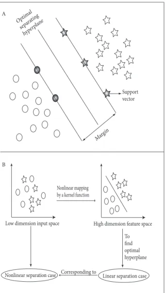
SVM originated as an implementation of Vapnik’s structural risk minimization principle (Vapnik, 1995). In the 2-dimensional case, which could be linearly separable, the data are separated by a hyperplane defined by plenty of support vectors (grayed out) that are a subset of training data used to define the boundary between the 2 classes. The simplest model of SVM action is shown in Figure 2A, where a thick solid line between the 2 different classes (circles and stars) is placed by the SVM and the line is kept in such a way that the space between 2 thin straight lines (margin) is maximized. We often encounter nonlinearly separable data; the SVM solves this problem by mapping input data into a high-dimensional feature space using a kernel function. By using this method, it is possible to identify a hyperplane that allows linear separation, as shown in Figure 2B.
The linear boundary can be expressed as:
w . x + b = 0, (10)
where w is termed the weight vector and b is the bias. Assuming that the training data with t number of samples are represented by {xi, yi}, i = 1, 2, 3, …, t, we attempt to find a function f : Rn → (+1,–1) based on the training data. Here, n is the dimensionality of the vector and y ∈ (+1,–1) denotes the 2-class label.
In the linear separable case:
w . x + b ≤ –1, for all y ∈ –1. (12)
The 2 inequalities of Eqs. (11) and (12) can be combined as:
yi (w . x + b) ≥ 1 (13)
Hence, the maximal distance to the closest point is formulated as , which can be found by minimizing ||w||2 subject to the constraint of Eq. (13). The optimization
procedure uses Lagrange multipliers and quadratic programming optimization methods so that the problem becomes one of maximizing
(14) under constraints αi ≥ 0, i =1, 2, 3,…t. Here, are the nonnegative Lagrange multipliers.
In the nonlinear separable case:
The training data need to be mapped into a high-dimensional feature space using a kernel function K (xi, ej) ≡ Φ (xi) . Φ (xj) so that linear separation becomes feasible. In this case, a slack variable (, i =1, 2, 3,…, t) is introduced to write Eq. (13) as Eq. (15), and the optimization problem is stated by Eq. (16):
yi (w . xi + b)–1 + ζi ≥ 0, (15) . (16) Here, C is a penalty parameter of the error term: a large value of C means assigning high penalty to errors.
AAB TAD TPP TSP TAB . . . . . . . . . . . .
Data set Input layer Hidden layer Output layer
Sect. Chrysantha Sect. Tuberculata
Sect. Paracamellia
Adjust weights
AAD
TTL
Figure 1. Schematic diagram of BP-ANN for Camellia prediction used in this study.
Figure 2. Schematic of SVM model. Hyperplanes for linearly
separable data. Thin straight line passes through the support vectors (A). Mechanism of kernel function in SVM model. Hyperplanes for nonlinearly separable data and mapping of dataset by kernel function (B).
Margin Optim al separat ing hyperp lane Support vector
Low dimension input space High dimension feature space
Nonlinear mapping by a kernel function To find optimal hyperplane Linear separation case Nonlinear separation case Corresponding to
A
Accordingly, the kernel function plays a very important role in SVM classification. Four popular kernel functions are the following:
Linear: K (xi, ej) = xi xj. (17) Polynomial: K (xi, ej) = (γxi xj + r)d, γ > 0. (18) Radial basis function (RBF):
K (xi, ej) = exp(γ⎪⎪xi xj ⎪⎪)2, γ > 0. (19) Sigmoid: K (xi, ej) = tanh(γxi xj + r). (20) Here, (default = 0) and d are kernel parameters. Thus, the problem could be solved by using a kernel function in the following classifier:
. (21)
C-SVM algorithms were designed and programmed under MATLAB software with the computer operating system of Windows XP. SVM algorithms were implemented with LIBSVM (Version 3.0), which is a library for support vector machines (http://www.csie.ntu.edu.tw/~cjlin/ libsvm). The time for manual and automatic classifications at date is less than 80 s.
3. Results
3.1. BP-ANN and SVM models
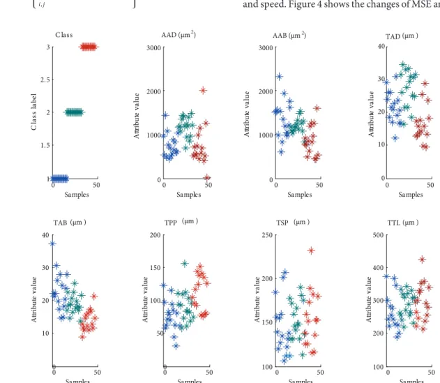
In this study, 47 species (samples) were used in total: 25 training set samples were used as the model and the remaining 22 samples were used in the prediction phase. The 47 samples were divided into 3 categories, and 7 feature attributes of samples were introduced, as seen in Figure 3. Table 1 shows the list of species that were presented to the models.
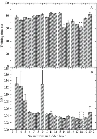
The optimum number of neurons in the hidden layer is selected by experimentation based on learning accuracy and speed. Figure 4 shows the changes of MSE and training
Figure 3. Samples divided into 3 categories and the data of 7 feature attributes of samples. Adaxial epidermal cell (AAD), thickness of
adaxial epidermal cell (TAD), thickness of palisade parenchyma (TPP), thickness of total leaf (TTL), thickness of spongy parenchyma (TSP), thickness of abaxial epidermal cell (TAB), and area of abaxial epidermal cell (AAB).
0 50 1 1.5 2 2.5 3 Samples Cl ass la be l C lass 0 50 0 1000 2000 3000 Samples A ttr ib ut e va lu e AAD (μm ) 0 50 0 1000 2000 3000 Samples A ttr ib ut e va lu e 0 50 0 10 20 30 40 Samples A ttr ib ut e va lu e TAD 0 50 0 10 20 30 40 Samples A ttr ib ut e va lu e TAB 0 50 0 50 100 150 200 Samples A ttr ib ut e va lu e TPP 0 50 100 150 200 250 Samples A ttr ib ut e va lu e TSP 0 50 100 200 300 400 500 Samples A ttr ib ut e va lu e TTL 2 AAB (μm )2 (μm ) (μm ) (μm ) (μm ) (μm )
time during the prediction with different numbers of neurons in the hidden layer. Our results indicate that the optimal number of nodes in the hidden layer is 18. Thus, a 7-18-3 back-propagation network was constructed.
In order to obtain good performance, some SVM parameters such as regularization parameter (C) and kernel parameter (γ) must be optimized by cross-validation. In
our work, lg2C and lg2γ were arranged from –5 to 5 with
an increment of 0.5. Hence, 21 lg2C and lg2γ values (–5,
–4.5, –4, –3.5, –3, –2.5, –2, –1.5, –1, –0.5, 0, 0.5, 1, 1.5, 2, 2.5, 3, 3.5, 4, 4.5, 5) were optimized simultaneously by cross-validation. The optimal SVM model was determined based on the highest accuracy. It can be observed in Figure 5 that the highest accuracy of 84.00% was achieved when C Table 1. Categories and classification of experimental samples from 3 sections of Camellia.
Categories Classification Training set Test set and no.
Sect. Chrysanthae 1 C. nitidissima C. longgangensis (1) 1 C. lungzhouensis C. impressinervis (2) 1 C. multipetala C. fusuiensis (3) 1 C. liomonia C. grandis (4) 1 C. euphlebia C. pingguoensis (5) 1 C. achrysantha C. pinggaoensis (6) 1 C. liberofilamenta C. limonia (7) 1 C. huana C. parvipetala (8) Sect. Tuberculata 2 C. tuberculata C. acuticalyx (9) 2 C. lipingensis C. atuberculata (10) 2 C. rhytidocarpa C. obovatifolia (11) 2 C. rhytidophylla C. rubimuricata (12) 2 C. leyeensis C. parvimuricata (13) 2 C. anlungensis C. hupehensis (14) 2 C. rubituberculata C. zengii (15) 2 C. acutiperulata C. pyxidiacea (16) Sect. Paracamellia 3 C. grijsii C. puniceiflora (17) 3 C. confuse C. tenii (18) 3 C. kissi C. microphylla (19) 3 C. fluviatilis C. miyagii (20) 3 C. brevistyla C. odorata (21) 3 C. hiemalis C. phaeoclada (22) 3 C. obtusifolia 3 C. maliflora 3 C. shensiensis
= 32 and γ = 0.13. Subsequently, the best parameters were used to generate the final SVM model.
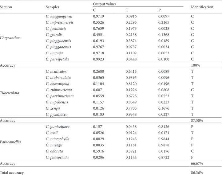
3.2. BP-ANN classification results
The confusion matrix (Table 2) shows the classification results of BP-ANN. Only 3 analyses were misclassified, thus obtaining the total accuracy of 86.36%. The classification of Sect. Chrysanthae by BP-ANN was the best with a 100% accuracy rate. Species Camellia rubimuricata Chang belonging to Sect. Tuberculata was incorrectly identified, showing it as a Sect. Chrysanthae member. Furthermore,
Camellia tenii and C. odorata from Sect. Paracamellia were
incorrectly identified as belonging to Sect. Tuberculata and Sect. Chrysanthae, respectively. The classification accuracies of Sect. Tuberculata and Sect. Paracamellia were 87.50% and 66.67%, respectively.
3.3. SVM classification results
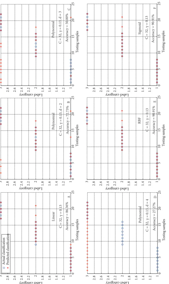
Linear, polynomial, RBF, and sigmoid classifiers were trained and tested using the kernels given by Eqs. (17) through (20), respectively. The polynomial degree (d) was the combination of the parameters of polynomial SVM with d∈ {2,3,4}. Figure 6 shows the classification results of different SVMs with optimal parameters. The RBF SVM
classifier and the sigmoid SVM classifier are better than the linear and polynomial SVM classifiers with 90.91% correct classification accuracy (Figure 6). The accuracy reached 100% for the first 16 samples from Sect. Chrysanthae and Sect. Tuberculata. However, the last 6 samples (from Sect.
Paracamellia), No. 18 (C. tenii), and No. 21 (C. odorata)
were incorrectly classified as Sect. Tuberculata, reducing the classification accuracy of Sect. Paracamellia to 66.67%. Additionally, the polynomial classifier becomes a linear SVM classifier when polynomial degree d is 1. As seen from Figures 6A–6D, in the 4 kinds of polynomial classifiers, the linear SVM (polynomial degree d = 1) achieved the best identification accuracy of 3 categories (86.36%) and the accuracy rate decreased as the polynomial degree increased (86.36%, 72.73%, 50.00%, and 27.27%).
4. Discussion
4.1. Potential usability
Camellia is commercially the most important genus of
the family Theaceae. It has been difficult to select suitable features for accurate classification of different species within this genus as there is great diversity at the section level. However, leaf characteristics have been frequently used to address inconsistencies in Camellia classification (Yang and Qi, 2005). With the rapid development of science and technology and increasing interdisciplinary research, the application of combination tools (such as Fourier transform infrared spectroscopy, random amplified polymorphic DNA, or numerical methods) with leaf anatomical data to solve classification discrepancies is very advantageous. In the present paper, for the first time, we employed 2 supervised pattern recognition techniques (BP-ANN and SVM) to achieve high classification accuracy when classifying Camellia species, especially using the RBF-SVM classifier in comparison with the
Camellia taxonomic systems of Chang (1998). Compared
with other methods, such as the LVQ classifier and DAN2 classifier used by Lu et al. (2012), the RBF-SVM classifier in our study produces a more accurate result. The techniques, like methods and accuracies of systems, used in classification of fruits and vegetables are various (Guyer and Yang, 2000; Moshou et al., 2003; Zheng et al., 2010), but it is difficult for accuracies to reach the classification results of RBF-SVM used in our study. The results show that leaf anatomical analysis using RBF-SVM can be effectively used to distinguish the genus Camellia. Moreover, flora guides like those of Chang (1998) and Ming (2000) are commonly used as a comprehensive resource to identify Camellia plants (Lu et al., 2012). However, the traditional information retrieval processes sometimes can be subjective. Thus, the methods used in this research could be regarded as extra but effective tools to classify new unknown species.
A
B
No. neurons in hidden layer
MSE Tr ai ni ng time (s ) 0 20 40 60 80 100 2 3 4 5 6 7 8 9 10 11 12 13 14 15 16 17 18 19 20 21 0.00 0.02 0.04 0.06 0.08 0.10 0.12 0.14 0.16 0.18
Figure 4. Mean squared error (MSE) and training time of the
Camellia training model with different numbers of neurons in the hidden layer.
Table 2. Output values and identification accuracy of the supervised BP-ANNa.
Section Samples Output values Identification
C T P Chrysanthae C. longgangensis 0.9719 0.0916 0.0097 C C. impressinervis 0.5526 0.2295 0.2165 C C. fusuiensis 0.7659 0.1973 0.0028 C C. grandis 0.4551 0.2138 0.1368 C C. pingguoensis 0.6193 0.3874 0.0189 C C. pinggaoensis 0.9767 0.0737 0.0034 C C. limonia 0.9718 0.1102 0.0053 C C. parvipetala 0.9923 0.0448 0.0100 C Accuracy 100% Tuberculata C. acuticalyx 0.2680 0.6413 0.0089 T C. atuberculata 0.0365 0.9395 0.0096 T C. obovatifolia 0.1104 0.8120 0.0196 T C. rubimuricata 0.6071 0.1226 0.0808 C C. parvimuricata 0.0559 0.6725 0.0553 T C. hupehensis 0.1157 0.8549 0.0223 T C. zengii 0.0126 0.7703 0.1676 T C. pyxidiacea 0.0183 0.9348 0.0227 T Accuracy 87.50% Paracamellia C. puniceiflora 0.1571 0.0438 0.8126 P C. tenii 0.0526 0.9124 0.0171 T C. microphylla 0.0029 0.1243 0.9844 P C. miyagii 0.0035 0.1181 0.9878 P C. odorata 0.5916 0.3721 0.0176 C C. phaeoclada 0.0286 0.1144 0.8722 P Accuracy 66.67% Total accuracy 86.36%
a: Columns C, T, and P contain the output neurons corresponding to sections of Chrysanthae (C), Tuberculata (T), and Paracamellia (P). –5 0 5 –5 0 5 30 40 50 60 70 80 90 100 log2 C log2 γ A ccu ra cy (% )
Figure 5. Classification accuracy in different kernel parameter (C) and regularization parameter (γ) by cross-validation in Camellia
0 5 10 15 20 25 1 1. 2 1. 4 1. 6 1. 8 2 2. 2 2. 4 2. 6 2. 8 3 Testing sample s Label category
Actual classification Predicted classification
0 5 10 15 20 25 1 1. 2 1. 4 1. 6 1. 8 2 2. 2 2. 4 2. 6 2. 8 3 Testing samples Label category 0 5 10 15 20 25 1 1. 2 1. 4 1. 6 1. 8 2 2. 2 2. 4 2. 6 2. 8 3 Testing samples Label category 0 5 10 15 20 25 1 1. 2 1. 4 1. 6 1. 8 2 2. 2 2. 4 2. 6 2. 8 3 Testing sample s Label category 0 5 10 15 20 25 1 1. 2 1. 4 1. 6 1. 8 2 2. 2 2. 4 2. 6 2. 8 3 Testing samples Label category 0 5 10 15 20 25 1 1. 2 1. 4 1. 6 1. 8 2 2. 2 2. 4 2. 6 2. 8 3 Testing samples Label category A B C D E F C = 32, γ = 0.13 C = 32, γ = 0.13, d = 2 C = 32, γ = 0.13, d = 3 C = 32, γ = 0.13, d = 4 C = 32, γ = 0.13 C = 32, γ = 0.13 Line ar Polynomi al Polynomi al Po lynomi al RB F Si gm oi d Ac curac y = 50.00% Ac curacy = 72.73% Ac curacy = 86.36% Ac curac y = 27.27% Ac curac y = 90.91% Ac curac y = 90.91%
Figure 6. The classification results of (A) linear, (B, C, and D) polynomial, (E) RBF, and (F) sigmoid SVM classifiers with the optimal
4.2. Effectiveness of BP-ANN and SVM model
The main aim of this study was to evaluate the feasibility of identifying species from the various sections of Camellia by supervised pattern recognition techniques (BP-ANN and SVM) and to determine their ability to assign species to respective sections. Both the BP-ANN and SVM models were developed using the same training data shown in Table 1. The BP-ANN architecture was a standard network, with 1 hidden layer, including 18 nodes with additional direct connections from 7 input neurons to 3 output neurons (7-18-3). An 86.36% total correct classification accuracy was achieved by BP-ANN. The supervised BP-ANN correctly identified all the species in Sect. Chrysanthae, with no errors in the prediction data, indicating that BP-ANN has strong ability to identify and assign species from sect. Chrysanthae. This conclusion validates Chang’s view on the close evolutionary relationship of species in sect. Chrysanthae. The discrimination power of the other 2 sections was relatively lower, as shown in Table 1. C. rubimuricata was separated into sect. Chrysanthae, and Camellia tenii and Camellia odorata were assigned to sect. Tuberculata and sect. Chrysanthae, respectively. The classification results of those 2 species in sect.
Paracamellia obtained from SVM were also incorrectly
identified, which indicated that Camellia tenii and C. odorata are similar to the other 2 sections. Taxonomy
itself is a dynamic discipline and no theory can support 100% accurate classification of any species. We should also note that deviation from the classification needs to be further investigated to see if a misclassification is due to the underlying algorithm’s fitting of data. Some misclassified species may indeed have underlying links in biological evolutionary principles with species of other sections. Therefore, we propose the possible misallocation of these species and the need for further research into their biological evolution. On the other hand, BP-ANN did not reach 100% classification accuracy for genus
Camellia, but the performance of the BP-ANN could be
improved by adding more characteristics and attributes as input. One hidden layer is usually sufficient for ANNs to approximate any nonlinear function (Hagan and Menhaj, 1994); thus, the use of a single hidden layer in our study is reasonable. In comparison, SVM classification resulted
in models showing slightly higher prediction accuracy (Figure 6). The optimal SVM model was determined by cross-validation; we selected the best parameters, C = 32, γ = 0.13, for SVM classifiers. As seen from the whole in Figure 6, the RBF SVM classifier and sigmoid SVM classifier are better than the polynomial SVM classifier for identification results. Since the polynomial SVM classifier becomes a linear SVM classifier when the polynomial degree d is 1, the linear SVM classifier achieves the best identification accuracies among polynomial SVM classifiers. In fact, the improvement in the classification accuracy is not much when the polynomial degree is more than 2.
Compared to the BP-ANN, the SVM has some advantages. The BP-ANN approach is based on the empirical risk minimization principles and suffers from the problem of over-fitting. However, the global optimum can be derived by SVM and the over-fitting model can be easily controlled by the choice of a suitable margin. Therefore, SVM possess excellent generalization in theory, which gets a better performance than the BP-ANN model in prediction set. Taking into account the accuracy of these 2 systems, it can be concluded that supervised pattern recognition techniques are valuable tools for taxonomic classification of Camellia species.
In conclusion, leaf anatomy data based on 7 attributes of 47 Camellia species were initially input to construct 2 classification models, BP-ANN and SVM. The overall results demonstrate that leaf anatomy data coupled with SVM can reliably classify different Camellia species into respective sections. Compared to BP-ANN, the SVM shows better classification accuracy. It can therefore be concluded that the use of leaf anatomy data together with a SVM has a high potential to classify species from different sections of Camellia, or potentially can be used for classification of other plant taxa.
Acknowledgments
This study was supported by grants from the Science and Technology Research Plan of Jinhua, China (No. 2009-2-020). The authors are grateful to Mr Dai Haibin, Mr Peng Qiufa, and Mr Pi Erxu for collecting living species and for technical assistance in leaf anatomy.
References
Bila S, Harkouss Y, Ibrahim M, Rousset J, N’Goya E, Baillargeat D, Verdeyme M, Aubourg M, Guillon P (1999). An accurate wavelet neural-network-based model for electromagnetic optimization of microwave circuits. Int J RF Micro CE 93: 297–306.
Burges CJC (1998). A tutorial on support vector machines for pattern recognition. Data Min Knowl Disc 2: 121–167.
Chang HT (1998). Camellia. In: Zhengyi W, Raven PH, editors. Flora of China. Beijing, China: Science Press, pp. 367–412.
Chen QS, Zhao JW, Fang CH, Wang DM (2007). Feasibility study on identification of green, black and Oolong teas using near-infrared reflectance spectroscopy based on support vector machine (SVM). Spectrochim Acta Part A 66: 568–574.
Chen QS, Zhao JW, Lin H (2009). Study on discrimination of roast green tea (Camellia sinensis L.) according to geographical origin by FT-NIR spectroscopy and supervised pattern recognition. Spectrochim Acta Part A 72: 845–850.
Cortes C, Vapnik V (1995). Support-vector networks. Mach Learn 20: 273–297.
Cybenco G (1989). Approximation by superposition of a sigmoidal function. Math Control Signal 2: 303–314.
Dogan A, Demirpence H, Cobaner M (2008). Prediction of groundwater levels from lake levels and climate data using ANN approach. Water SA 34: 1–10.
Giacomini M, Ruggiero C, Calegari L, Bertone S (2000). Artificial neural network based identification of environmental bacteria by gas-chromatographic and electrophoretic data. J Microbiol Meth 43: 45–54.
Guyer D, Yang X (2000). Use of genetic artificial neural networks and spectral imaging for defect detection on cherries. Comput Electron Agr 29: 179–194.
Hagan MT, Menhaj MB (1994). Training feed forward networks with the Marquardt algorithm. IEEE T Neural Networks 6: 861–867 Hornik K, Stinchombe M, White H (1989). Multilayer feed forward
network are universal approximator. Neural Networks 2: 359– 366.
Jiang B, Peng QF, Shen ZG, Moller M, Pi EX, Lu HF (2010). Taxonomic treatments of Camellia (Theaceae) species with secretory structures based on integrated leaf characters. Plant Syst Evol 290: 1–20.
Jiang W, Nitin M, Jiang B, Zheng YP, Hong SS, Lu HF (2012). Floral morphology resolves the taxonomy of Camellia L. (Theaceae) sect. Oleifera and sect. Paracamellia. Bangl J Plant Taxon 19(2): 155–165.
Kong HZ (2001). Comparative morphology of leaf epidermis in the Chloranthaceae. Bot J Linn Soc 136: 279–294.
Kumar V, Kodandaramaiah J, Rajan MV (2012). Leaf and anatomical traits in relation to physiological characteristic in mulberry (Morus sp.) cultivars. Turk J Bot 36: 683–689.
Li ZX, Yang XM (2008). Damage identification for beams using ANN based on statistical property of structural responses. Comput Struct 86: 64–71.
Lin XY, Peng QF, Lv HF, Du YQ, Tang BY (2008). Leaf anatomy of Sect.
Oleifera Chang and Sect. Paracamellia Sealy and its taxonomic
significance. J Syst Evol 46: 183–193.
Lu H, Jiang W, Ghiassi M, Lee S, Nitin M (2012). Classification of
Camellia (Theaceae) species using leaf architecture variations
and pattern recognition techniques. PLoS ONE 7: e29704. Lu HF, Jiang B, Shen ZG, Shen JB, Peng QF, Cheng CG (2008).
Comparative leaf anatomy, FTIR discrimination and biogeographical analysis of Camellia section Tuberculata (Theaceae) with a discussion of its taxonomic treatments. Plant Syst Evol 274: 223–235.
Lu HF, Pi EX, Peng, QF, Wang LL, Zhang CJ (2009). A particle swarm optimization-aided fuzzy cloud classifier applied for plant numerical taxonomy based on attribute similarity. Expert Syst Appl 36: 9388–9397.
Lu HF, Shen JB, Lin XY, Fu JL (2008). Relevance of Fourier transform infrared spectroscopy and leaf anatomy for species classification in Camellia (Theaceae). Taxon 57: 1274–1288.
Lu HF, Zheng H, Lou HQ, Jiang LL, Chen Y, Fang SS (2010). Using neural networks to estimate the losses of ascorbic acid, total phenols, flavonoid, and antioxidant activity in asparagus during thermal treatments. J Agr Food Chem 58: 2995–3001.
Luo D, Hosseini HG, Stewart JR (2004). Application of ANN with extracted parameters from an electronic nose in cigarette brand identification. Sensors Actuat B 99: 253–257.
Ming TL (2000). Monograph of the Genus Camellia. Kunming, Yunnan, China: Science and Technology Press.
Mitchell TM (1997). Machine Learning. Boston: WCB/McGraw-Hill. Moshou D, Wahlen S, Strasser R, Schenk A, De Baerdemaeker J,
Ramon H (2005). Chlorophyll fluorescence as a tool for online quality sorting of apples. Biosyst Eng 91: 163–172.
Pi EX, Lu HF, Jiang B, Huang J, Peng QF, Lin XY (2011). Precise plant classification within genus level based on simulated annealing aided cloud classifier. Expert Syst Appl 38: 3009–3014.
Pi EX, Peng QF, Lu HF, Shen JB, Du YQ, Huang FL, Hu H (2009). Leaf morphology and anatomy of section Camellia (Theaceae). Bot J Linn Soc 3: 456–476.
Pontil M, Verri A (1998). Support vector machines for 3-D object recognition. IEEE T Pattern Anal 20: 637–646.
Roggo Y, Duponchel L, Huvenne LP (2003). Comparison of supervised pattern recognition methods with McNemar’s statistical test: Application to qualitative analysis of sugar beet by near-infrared spectroscopy. Anal Chim Acta 477: 187–200.
Sadeghi BHM (2000). A BP-neural network predictor model for plastic injection molding process. J Mater Process Tech 103: 411–416. Shen JB, Lu HF, Peng QF, Zheng JF, Tian YM (2008). FTIR spectra of
Camellia sect. Oleifera, sect. Paracamellia, and sect. Camellia
(Theaceae) with reference to their taxonomic significance. J Syst Evol 46: 194–204.
Turhan K, Serdar B (2013). Support vector machines in wood identification: the case of three Salix species from Turkey. Turk J Agric For 37: 249–256.
Vapnik VN (1989). Statistical Learning Theory. New York: Wiley. Vapnik VN (1995). The Nature of Statistical Learning Theory. New
York: Springer.
Vasic PS, Dubak DV (2012). Anatomical analysis of red Juniper leaf (Juniperus oxycedrus) taken from Kopaonik Mountain, Serbia. Turk J Bot 36: 473–479.
Vijayan K, Zhang WJ, Tsou CH (2009). Molecular taxonomy of
Camellia (Theaceae) inferred from nrITS sequences. Am J Bot
96: 1348–1360.
Yang ZR, Qi L (2005). Comparative morphology of the leaf epidermis in Schisandra (Schisandraceae). Bot J Linn Soc 148: 39–56. Yuan SF, Chu FL (2007). Fault diagnostics based on particle swarm
optimization and support vector machines. Mech Syst Signal Pr 21: 1787–1798.
Zheng H, Fang SS, Lou HQ, Chen Y, Jiang LL, Lu HF (2011). Neural network prediction of ascorbic acid degradation in green asparagus during thermal treatments. Expert Syst Appl 38: 5591–5602.
Zheng H, Lu HF, Zheng YP, Lou HQ, Chen CQ (2010). Automatic sorting of Chinese jujube (Zizyphus jujuba Mill. cv. ‘hongxing’) using chlorophyll fluorescence and support vector machine. J Food Eng 101: 402–408.