Robotic assembly line design with tool changes

(1)

ROBOTIC ASSEMBLY LINE DESIGN WITH

TOOL CHANGES

a thesis

submitted to the department of industrial engineering

and the institute of engineering and science

of bilkent university

in partial fulfillment of the requirements

for the degree of

master of science

By

Adnan Tula

(2)

Prof. Dr. M. Selim Akt¨urk (Advisor)

I certify that I have read this thesis and that in my opinion it is fully adequate, in scope and in quality, as a thesis for the degree of Master of Science.

Prof. Dr. Erdal Erel

I certify that I have read this thesis and that in my opinion it is fully adequate, in scope and in quality, as a thesis for the degree of Master of Science.

Assoc. Prof. Dr. Oya Ekin Kara¸san

Approved for the Institute of Engineering and Science:

Prof. Dr. Mehmet B. Baray Director of the Institute

(3)

ABSTRACT

ROBOTIC ASSEMBLY LINE DESIGN WITH TOOL

CHANGES

Adnan Tula

M.S. in Industrial Engineering Supervisor: Prof. Dr. M. Selim Akt¨urk

July, 2009

This thesis is focused on assembly line design problems in robotic cells. The mixed-model assembly line design problem that we study has several subprob-lems such as allocating operations to the stations in the robotic cell and satisfying the demand and cycle time within a desired interval for each model to be pro-duced. We also ensure that assignability, precedence and tool life constraints are met. The existing studies in the literature overlook the limited lives of tools that are used for production in the assembly lines. Furthermore, the studies in the literature do not consider the unavailability periods of the assembly lines and assume that assembly lines work 24 hours a day continuously. In this study, we consider limited lives for the tools and hence we handle tool change decisions. In order to reflect a more realistic production environment, we deal with designing a mixed-model assembly line that works 24 hours a day in three 8-hour shifts and we consider lunch and tea breaks that are present in each shift. This study is the first one to propose using such breaks as tool change periods and hence eliminate tool change related line stoppages. In this setting, we determine the number of stations, operation allocations and tool change decisions jointly. We provide a heuristic algorithm for our problem and test the performances of our heuristic algorithm and DICOPT and CPLEX solvers included in GAMS software on different instances with varying problem parameters.

Keywords: Robotic cell, assembly line, tool change, heuristic algorithm. iii

(4)

UC

¸ DE ˘

G˙IS

¸ ˙IML˙I ROBOT˙IK MONTAJ HATTI TASARIMI

Adnan Tula

Endüstri Mühendisli˘gi, Yüksek Lisans Tez Yöneticisi: Prof. Dr. M. Selim Aktürk

Temmuz, 2009

Bu tezin konusu robotik hücrelerde montaj hattı tasarım problemleridir. Ç alı¸stı˘gımız montaj hattı tasarım problemi operasyonların istasyonlara atan-ması ve üretilecek her model i¸cin talep ve ¸cevrim zamanının belli aralıklar i¸cinde kar¸sılanması gibi alt problemler i¸cermektedir. Bunun yanı sıra atan-abilirlik, öncelik ve u¸c ömrü kısıtları sa˘glanmaktadır. Literatürde var olan ¸calı¸smalarda, montaj hatlarında üretim i¸cin kullanılan u¸cların kısıtlı ömrü oldu˘gu gözardı edilmi¸stir. Ayrıca, literatürde yer alan ¸calı¸smalar 24 saat kesintisiz ¨

uretimi temel almakta ve montaj hatlarında üretim yapılamayan zamanlar hesaba katılmamaktadır. Bu tezde, kısıtlı u¸c ömürleri kullanılmakta, dolayısıyla u¸c de˘gi¸sim kararları da ele alınmaktadır. Daha ger¸cek¸ci bir üretim ortamı yansıtmak amacıyla, karma model üretimi yapılan, i¸cinde ¸cay ve yemek molalarının oldu˘gu 8 saatlik ü¸c vardiya düzeniyle günde 24 saat ¸calı¸san bir montaj hattı tasarım problemi ele alınmı¸stır. Bu ¸calı¸sma, ¸cay ve yemek molalarının u¸c de˘gi¸stirme zamanı olarak kullanılmasını ve bunun sonucunda u¸c de˘gi¸sim zorunlulu˘gundan kaynaklanan üretim hattı durdurmalarının önlenmesini önermesi a¸cısından ilk-tir. Bu ba˘glamda, istasyon sayıları, operasyonların istasyonlara atanması ve u¸c de˘gi¸sim kararları birlikte ele alınmaktadır. Ç alı¸sılan problem i¸cin ¸cözüm yolu olarak bir sezgisel algoritma geli¸stirilmi¸s, de˘gi¸sken de˘gerlerin atandı˘gı parame-trelerle olu¸sturulan de˘gi¸sik örnekler üzerinde sezgisel algoritma ile DICOPT ve CPLEX ¸cözücülerinin performansları kar¸sıla¸stırmalı olarak test edilmi¸stir.

Anahtar sözcükler: Robotik hücre, montaj hattı, u¸c de˘gi¸simi, sezgisel algoritma. iv

(5)

To my father...

(6)

First and foremost, I would like to express my gratitude to my advisor, Prof. Dr. M. Selim Akt¨urk, for his invaluable guidance and helps during my M.S. study. With his support and advices, he has always been more than an advisor to me.

I am also grateful to Prof. Dr. Erdal Erel and Assoc. Prof. Dr. Oya Ekin Kara¸san for accepting to read and review this thesis and for their invaluable suggestions.

I would like to express my deepest gratitude to my father, H¨useyin Tula and my mother, Necla Tula for their endless love, encouragement and support. I have always felt very lucky that I am their child, and I will always do my best to keep them feeling the same for me.

I am indebted to all my friends who were always with me and made my life more beautiful. I am especially grateful to ˙Ihsan Yanıko˘glu, Utku Guru¸s¸cu, Könül Bayramo˘glu, Safa Onur Bingöl, Merve Ç elen, Onur Özkök, Sibel Alumur, Duygu Tutal, Ezel Ezgi Budak and Ceyda Kırık¸cı for everything they have done for me. Finally, I would like to express my special thanks to T ÜB˙ITAK for the schol-arship provided throughout the thesis study. The research was partially sup-ported by Tofa¸s Türk Otomobil Fabrikası A.S¸. (Fiat Turkey) as Bilkent Univer-sity Project No: 300 189 2 5.

(7)

List of Tables

4.1 Precedence matrix for Example 1 . . . 25

4.2 Precedence matrix for Example 3 . . . 34

6.1 Precedence matrix for computational study runs . . . 44

6.2 Total Profit Values for Algorithm 1 and Algorithm 2 . . . 45

6.3 Calculation of Total Profit Values for Algorithm 1 and Algorithm 2 46 6.4 Total Profit Values for DICOPT 1 and MIP 1 . . . 47

6.5 Total Profit Values for DICOPT 2 and MIP 2 . . . 48

6.6 Gap values for MIP 1 and MIP 2 . . . 49

6.7 Total Profit Values and CPU Times for CPLEX and Algorithm 2 50 6.8 Solution Analysis for Problem Clusters . . . 51

(10)

Introduction

An important application of robots in the automotive industry is their use for spot welding operations in robotic cells. Once an automotive component of a vehicle is designed and the required spot welds to assemble the pieces on this component are determined, the problem of allocating the welding operations to robotic cell stations arises. Different allocations result in different production quantities (e.g., cycle times), station investment costs and tooling costs that are incurred by replacing the tools with new ones. Each station consists of a single robot in a fully automated production line. In order to perform welding operations, the robots use spot welding guns that we refer to as welding tools throughout this study. A welding tool has a limited life time that is represented by the total number of spot welds that it can process.

This study focuses on a robotic cell mixed-model assembly line design problem in which multiple models can be produced in any order. Our objective is to maxi-mize the total profit that will be gained from the assembly line by manufacturing automotive body components. The problem has several subproblems which in-clude allocation of welding operations to the stations, satisfying the demand and cycle time within a desired interval for the parts to be produced. While defining the problem and constraints, we were inspired by a real-life assembly line problem we faced in a project that we formerly conducted at one of the leading companies in the automotive industry in Turkey.

(11)

CHAPTER 1. INTRODUCTION ₂

Today, improvements in technology and automation and large investment costs incurred for building assembly lines have increased the importance of studies on designing efficient assembly lines. Assembly line designing problems attract much attention from the academic world. Therefore, numerous studies have been conducted by the researchers, in which some aspects such as equipment selection and balancing of the lines are considered.

1.1 Literature Review

As described by Baybars [3], there are two main groups of assembly line studies. Simple assembly line balancing problems (SALBP) consider a single product to be produced in the assembly lines. In the literature, the widely used objectives for these studies include minimizing the number of workstations or the cost for building assembly lines for a given cycle time and minimizing the cycle time for a given number of workstations. There are many studies in the field of SALB, some of which are Baybars [2], McMullen and Tarasewich [16], Fleszar and Hindi [10], Rekiek et al. [19], Scholl and Klein [22] and Levitin et al. [14]. For a review of studies in the SALB field, we can refer to the review paper of Scholl and Becker [21].

In general assembly line balancing problems (GALBP), SALB problems are extended by introducing other aspects such as mixed-model or multi-model cases, zoning constraints and parallel stations. As described by Becker and Scholl [4], in a mixed-model line, different models are produced in the assembly line in an arbitrary inter-mixed sequence. There are several studies in the literature for the version of assembly line balancing problem with mixed-model lines. Bukchin et al. [5] address the problem of designing mixed-model assembly lines in which a make-to-order policy is followed. By separating the assembly tasks into two sets, they propose a three-stage heuristic in order to find a solution with the minimum number of stations for a given cycle time: in the first stage, they assign the first set of tasks that should be assigned to the same station for each model requiring these tasks. Then, they assign the second set of tasks that can be assigned to

(12)

different stations for different models to balance each model in the assembly line, subject to the constraints resulting from the assignment of the first set of tasks. The final stage is to improve the solution by a neighborhood search. Erel and G¨okcen [7] use a shortest-route formulation to solve a mixed-model assembly line problem. Common assembly tasks between different models are assigned to the same station. They transform the problem into a single-model version by constructing a combined precedence diagram from the precedence diagrams of all models. Bukchin and Rabinowitch [6] relax the assumption of restricting a task that is common for several models to a particular station and allow such a task to be assigned to different stations for different models. They provide an integer formulation for their model and give a lower bound for the total station cost and task assignment costs, which they aim to minimize. In order to find optimal or near-optimal solutions, they propose a heuristic algorithm based on branch-and-bound. Haq et al. [12] present a hybrid genetic algorithm for the mixed-model assembly line balancing problem. They use the modified ranked positional weight method to obtain an initial assignment of tasks to stations. They reduce the search space and search time of their hybrid genetic algorithm by providing this initial solution to their algorithm. Different from the studies that adapt a single station at each stage of the assembly line, Askin and Zhou [1] proposed a nonlinear integer program for assigning tasks to stations in a serial line in which the stages of the assembly line consist of an arbitrary number of identical, parallel workstations. While considering precedence relations between tasks, they allow tooling selections for workstations and each task requires a certain type of tool. Their objective is to minimize the sum of the total fixed cost for operating stations and the total equipment/tooling cost. Because of the complexity of the problem, they provide an assignment heuristic for finding good initial solutions.

To address the problem of handling model changes in mixed-model lines, Matanachai and Yano [15] approach the mixed-model line problem with the ob-jective of facilitating the construction of good sequences and short-term workload stability while assigning tasks to stations. They assume predetermined cycle times and number of stations and include additional terms in their objective function

(13)

CHAPTER 1. INTRODUCTION ₄

to minimize within- and between-station processing time diversity. Maintain-ing short-term workload stability provides robustness for daily model changes in mixed-model lines. Merengo et al. [17] present balancing and sequencing method-ologies for mixed-model assembly lines to minimize the number of workstations for predetermined model cycle times, reduce work-in-process and minimize the rate of incomplete jobs. By presenting integer programming formulations and providing numerical results, Sawik [20] compared monolithic and hierarchical balancing and sequencing approaches in which balancing and sequencing of mixed-model lines are determined simultaneously and sequencing of models proceeds the balancing of the line, respectively.

Sparling and Miltenburg [23] were the first to study the mixed-model U-line balancing problem to minimize the number of stations in the assembly line. For this problem, they presented a four-step approximate solution algorithm: the first two steps transform the mixed-model problem into an equivalent single-model problem, the third step finds the optimal workload balance for the equivalent single-model problem and the final step transforms the balance found in the third step into a feasible balance for the original mixed-model problem. Miltenburg [18] extended balancing and sequencing problem to U-shape mixed-model lines in a just-in-time environment. A nonlinear mixed-integer programming formulation is presented to solve the balancing and sequencing problem simultaneously. Erel et al. [8] developed a simulated annealing-based algorithm to minimize the num-ber of stations in a U-type assembly line and tested the performance of their proposed algorithm against optimum seeking DP and IP-based algorithms and other heuristic procedures. In contrast to deterministic processing times, Erel et al. [9] studied U-line balancing problem with stochastic task times. Their study was the first one to propose a beam search-based method to minimize total ex-pected cost, which consists of total labor cost and total exex-pected incompletion cost. Van Hop [13] addressed the mixed-model assembly line problem with fuzzy processing times for the first time. A heuristic to aggregate fuzzy processing times is proposed and the problem is transformed into a a single-model version by using a combined precedence diagram. A heuristic is also developed to find a solution for the fuzzy assembly line problem. Vilarinho and Simaria [24] address

(14)

some additional zoning constraints in their study for the assignment of tasks to stations. They assume a subset of tasks that are linked and must be assigned to the same station and subsets of incompatible tasks that should be assigned to different stations. They also assume that some tasks can only be assigned to particular stations. They allow parallel stations in the assembly line and present an ant colony optimization algorithm for minimizing the number workstations for a given cycle time. Wilhelm and Gadidov [25] devised a branch-and-cut approach to minimize the total assembly line cost that includes station activating, machin-ing and toolmachin-ing costs considermachin-ing machine capacities and available tool spaces in the stations. Each operation requires a set of tools to be performed so tooling requirements constitute an important part of the problem. Machine capacity is used as an analog of cycle time restriction that appears in single-model assembly lines.

The studies in the literature present different model formulations and propose different solution techniques for assembly line problems with different objective functions. However, these studies do not consider the unavailability periods of the assembly lines and hence are based on continuous production. In addition to this, they overlook the limited lives of the tools that are used in production. As we will further discuss in Chapter 5, assembly lines may suffer from tool change related line stoppages unless the limited tool lives are taken into consideration while allocating the operations to the stations. Therefore, we consider these two important attributes of the robotic assembly lines in addition to other well-known constraints of the assembly line balancing problem.

1.2 Thesis Overview

Traditional assembly line design studies are generally based on the objectives of minimizing the cycle time, the number of stations and costs for building as-sembly lines or maximizing the efficiency of the asas-sembly lines. In this study, different from the studies in the literature, we address a mixed-model assembly line problem with a profit maximization objective. We maximize the total profit

(15)

CHAPTER 1. INTRODUCTION ₆

function, which is the difference between the revenue gained by manufacturing components of the final products and the sum of the station investment costs and tooling costs. Station investment costs include robot cost, fixture cost and space cost and tooling costs are incurred by replacing the tools with new ones. In addition to this, the studies in the literature do not consider the unavailability periods of the assembly lines and assume that assembly lines work 24 hours a day continuously. However, we deal with designing a mixed-model assembly line that works 24 hours a day in three 8-hour shifts. We consider lunch and tea breaks to reflect a more realistic production environment. In the literature, there are many studies regarding tool selection and tool costs, but these studies ignore limited tool life and incorporate the assumption that tool change is omitted throughout the planning horizon and tooling costs are incurred once at the beginning of the production stage. Tool life has two implications. First, tools must be changed at the end of their tool lives and this will increase the tooling cost. Second, tool changes may correspond to a time when the assembly line is supposed to be op-erating and therefore may result in line stoppages. In our study, we consider that tools have limited lives that are represented by the total number of spot welds that they can perform. We use the lunch and tea breaks as tool change periods by which we aim to eliminate tool change related line stoppages. At each break, if there exist welding tools that have a remaining number of spots less than the total number of spots that they have to perform until the next break, they should be changed with new ones. Therefore, the tooling cost term that appears in our objective function is a function of the total number of tools used throughout the planning horizon.

The organization of this study is as follows: In the next chapter we will present a nonlinear mixed-integer formulation of our assembly line design problem. In Chapter 3, we will provide the linearized mixed-integer version of the same prob-lem. In Chapter 4, a heuristic algorithm for finding good feasible solutions will be developed and this heuristic algorithm will be improved by a surrogate problem. An implementation of our study to a leading automotive company in Turkey will be provided in Chapter 5. Numerical results and several comparisons between our heuristic algorithm and GAMS software are given in Chapter 6. Concluding

(16)

remarks are given in Chapter 7. A summary of all the problem parameters and decision variables is provided in the appendix.

(17)

Chapter 2 Problem Definition

In this chapter, we give the definition of our problem and introduce the parame-ters, variables and the mathematical model we will use to solve our problem.

We consider a robotic cell that contains at most m stations: S1, S2, . . . , Sm.

Let M={1, 2,. . . , m} be the set of indices of these stations. Space restrictions in the production area and a limited budget for investment costs are among the reasons of such a restriction on the number of stations. We use the parameter Vj to denote the cost of setting up station j, j ∈ M. The cost of setting up a

station consists of robot cost, fixture cost and space cost. There are g different models of parts to be produced in this robotic cell and G={1, 2,. . . , g} is the index set of part models. Ohi represents operation i of model h, i ∈ Nh, h ∈ G,

where Nh={1, 2,. . . , nh} is the index set of welding operations of model h to

be allocated to stations and nh is the number of operations to be performed to

produce a part of model h. Welding operations consist of a number of spot welds. Let Whi be the number of spot welds required to perform operation i of model

h, i ∈ Nh, h ∈ G. An operation may require a single spot weld. However, some

operations require more than one spot weld in order to assemble the part at its proper geometry. In general, the spot welds that are close to each other with respect to their locations on the component are grouped together as operations. A welding tool has a limited lifetime that is represented by the total number of spot welds it can process. We define Bj as the total number of spot welds such

(18)

that the welding tool in station j ∈ M can process.

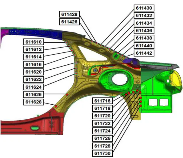
Figure 2.1: A spot weld scheme of an automotive body component

An example of an automotive body component is given in Figure 2.1. Figure 2.1 shows the spot welds required to perform some of the welding operations on different locations of a part. The 26 spot welds seen in this figure constitute a subset of all operations required to produce this body component. As we can see, a spot weld can be close to some spot welds but can also be distant from some other spot welds. Therefore, the locations of the spot welds on a part along with the minimum number of required spot welds to assemble the subcomponents to maintain their proper geometry during the part transfer between stations play an important role in grouping these spot welds as operations.

(19)

CHAPTER 2. PROBLEM DEFINITION ₁₀

In order to set up a profitable assembly line and determine the number of stations required in the assembly line, we have to take the expected demand into consideration. We represent the yearly expected demand for the parts to be produced as θh, h ∈ G. We use the parameter γh to denote the target cycle

time for model h to meet the yearly expected demand θh. In general, let ¯Th be

the time allocated to production of model h. Let ¯fh be the cycle time of model

h and let ¯θh be the corresponding production amount for model h. Then, the

relationship between ¯fh and ¯θh is as follows:

¯ θh = ¯ Th ¯ fh ∀h. We use the parameters γL

h and γhU as the lower and upper bounds for the actual

cycle time of model h, respectively. We neither accept to produce an amount of parts of model h less than the amount that can be produced when the actual cycle time is equal to γU

h nor can make any additional profit if production of model h

exceeds the amount that can be produced when the actual cycle time is equal to γL

h. Up to the production amount of θh we assume a constant profit for each

part of model h produced and denote it by P Rh. In case of producing between

θh and the amount that can be produced when the actual cycle time is equal to

γL

h, each excess part of model h produced contributes an expected profit denoted

by P Rǫ

h. If the production of model h exceeds the amount that can be produced

when the actual cycle time is equal to γL

h, any excess part does not contribute

any additional profit. We represent the relationship between P Rh and P Rǫh as

the following:

P R_hǫ = P Rh− ∆h, ∆h ≥ 0.

Let fh be the cycle time of model h for a particular allocation. Let bθh and θhL

be the production amounts of model h when the cycle time of model h is equal to the decision variable, fh, and the given parameter, γhL, respectively. In this

setting, revenue contribution of each model h, which is the sum of the individual profits that each product of model h contributes, is calculated as in the following:

Total Revenue =        b θh· P Rh if γh ≤ fh ≤ γhU, θh· P Rh+ (bθh− θh) · P Rǫh if γ L h ≤ fh ≤ γh, θh· P Rh+ (θLh − θh) · P Rǫh if fh < γhL.

(20)

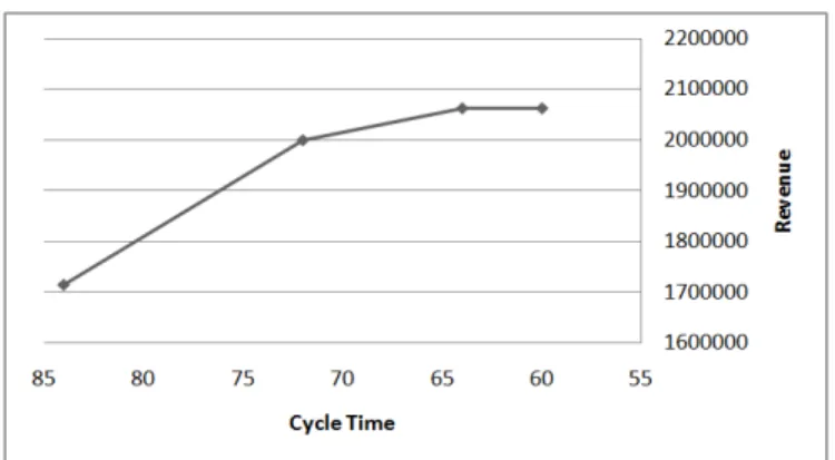
Figure 2.2 shows an example of the relationship between the revenue contri-bution such that P Rh = $20 and P Rhǫ = $5 and the cycle time for a particular

model h that is produced in the assembly line, where γU

h = 84 seconds, γh = 72

seconds and γL

h = 64 seconds.

Figure 2.2: Cycle time - revenue contribution relationship

As we see in Figure 2.2, while the cycle time of model h decreases from γU h

(i.e., 84 seconds) to γh (i.e., 72 seconds), the contribution of model h to the total

revenue increases with a slope of P Rh. While the cycle time decreases from γh

to γL

h (i.e., 64 seconds), the revenue increases with a slope of P Rǫh. The slope

between γh and γhL is lower than the slope between γhU and γh because after the

production amount of the expected demand θh, each excess component of model

h produced contributes an expected profit of P Rǫ

h, which is lower than P Rh.

Finally, when the cycle time decreases down from γL

h, the revenue contribution of

model h remains constant because after the production amount of θL

h, any excess

component of model h does not contribute any profit.

There are several reasons for an assembly line to stop when it is supposed to be operating. For instance, the tips of the welding tools may cling on the part during a welding operation and the welding tool then must be replaced with a new one. Also, the grippers used for transportation of parts through the assembly line may not close properly and therefore may not hold the part, which causes the assembly line to stop. Moreover, the censors may not recognize or may miscognize a part. In addition to these, a welding tool may finish its lifetime at some time when the assembly line is supposed to be operating. Except in the

(21)

CHAPTER 2. PROBLEM DEFINITION ₁₂

last instance, the reasons that cause the assembly line to stop are more technical and may happen at any time. However, the last instance can be prevented by making it possible to allow tool changes only in scheduled breaks such as tea or lunch breaks in which the assembly line does not operate.

In most of the automotive industries (including the one that we have been collaborating), plants work 24 hours in three 8-hour shifts and there are breaks in an 8-hour shift. In general, there is a 10-minute break at the beginning of a shift, a 10-minute tea break, a 30-minute lunch break and a second 10-minute tea break. The working hours between two breaks are equal and last 1 hour and 45 minutes. Each break corresponds to a possible tool change time period. In any break, if the remaining number of spots such that a welding tool can perform is less than the total number of spots it has to perform until the next break, it needs to be replaced with a new tool in that particular tool change time period in order to prevent line stoppages due to the tool changes. Let Cj be the cost of

the tool in station j, j ∈ M. We define Dq as the available tool change time in

tool change period q, q = 1, 2, . . . , U, where U is the total number of breaks in the planning horizon.

We calculate the required tool change time as a function of the number of tools to be replaced: K+ µ · m X j=1 zjq ∀q = 1, 2, . . . , U,

where K is a constant that denotes the time to prepare for welding tool changes and µ is another constant that corresponds to the time required to replace a single welding tool. Furthermore, zjq is a binary variable to indicate whether tool in

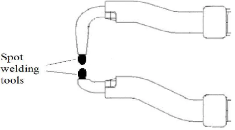
station j ∈ M is changed in tool change period q. Two spot welding tools are attached to the spot welding gun as shown in Figure 2.3, and both of them are replaced at the same time.

As we have previously seen in Figure 2.1, the positions of spot welds on a part are at different locations. It may not be possible for a particular type of welding tool to reach to every location on a part due to its geometry. Therefore, it is not possible to process all spot welds by one type of welding tool so there

(22)

Figure 2.3: A spot welding gun

are several types of welding tools. As a result, a welding tool cannot perform all operations so we define an assignability matrix A and use the following parameter:

ahij =       

1, if operation i ∈ Nh of model h ∈ G can be assigned

to station j ∈ M; 0, otherwise.

There may be additional subcomponents to be assembled to a part of model h inside the robotic cell. The subcomponents may block the positions of some spot welds required for an operation, i.e., Ohi. Therefore, Ohi must be performed

before this particular subcomponent is assembled to the part. For similar reasons, we define a precedence matrix P and use the following parameter:

phik =       

1, if operation i ∈ Nh of model h ∈ G precedes operation

k ∈ Nh of model h ∈ G;

0, otherwise.

The difference between the processing time of a spot weld by two different types of welding tools is negligible so the processing time of an operation is independent of the station at which it is processed. Therefore, we let thi be the

time required to perform operation i ∈ N of model h ∈ G. We calculate thi as a

(23)

CHAPTER 2. PROBLEM DEFINITION ₁₄

as follows:

thi = α + β · Whi ∀h ∈ G, i ∈ Nh,

where α is a constant that denotes the time required for the robot to reach to the position to perform operation i of model h and β is another constant that corresponds to the time required to process a single spot weld.

In order to calculate the time allocated for production of parts of a particular model, we need to calculate the proportion of time that should be allocated to the production of a particular model. Therefore we define the parameter ψh for

h= 1, . . . , g as the following: ψh = θh· γh Pg l=1θl· γl ∀h ∈ G.

As mentioned before, the production time between two breaks is 1 hour 45 min-utes, which is equal to 6300 seconds. Then, the time allocated for the production of parts of model h between two breaks in the assembly line is calculated as 6300 · ψh seconds.

The decision variables we will use to formulate our model are defined below: fh: actual cycle time for model h, h ∈ G.

σj =

(

1, if station j ∈ M is used in the assembly line; 0, otherwise.

xhij =

(

1, if operation i ∈ Nh of model h ∈ G is assigned to station j ∈ M;

0, otherwise. zjq =       

1, if tool in station j ∈ M is changed in tool change period q, q = 1, 2, . . . , U;

0, otherwise.

Rjq: remaining number of spot welds such that the welding tool in station j can

(24)

Having defined the parameters and the decision variables of our problem, the nonlinear mixed-integer mathematical model we will use to solve our problem is the following: Model 1 (NLMIP): Maximize g X h=1 P Rh· min{ θh· γh fh , θh} (2.1) + g X h=1 P Rǫ_h· min{max{θh · γh fh − θh,0}, θh· γh γL h − θh} − ρ · m X j=1 U X q=1 Cj · zjq− η · m X j=1 Vj· σj Subject to fh ≥ τj · σj + nh X i=1 thi· xhij ∀h, j (2.2) fh ≤ γhU ∀h (2.3) xhij ≤ ahij· σj ∀h, i, j (2.4) m X j=1 xhij = 1 ∀h, i (2.5) phik· j X l=1 xhil + (1 − phik) ≥ xhkj ∀h, i, j, k (2.6) Rjq= Bj · zjq+ [Rj(q−1)− g X h=1 6300 · ψh fh · nh X i=1 Whi· xhij](1 − zjq) ∀j, q (2.7) Rj0= Bj ∀j (2.8) Rjq≥ g X h=1 6300 · ψh fh · ( nh X i=1 Whi· xhij) ∀j, q (2.9) fh ≥ 0, Rjq ≥ 0, xhij, σj, zjq∈ {0, 1} ∀h, i, j, q (2.10)

We use a piecewise linear objective function in which we include the profit that is supposed to be earned by producing up to θh amount of parts of model h.

We add the extra profit for the situation of producing more than θh and subtract

(25)

CHAPTER 2. PROBLEM DEFINITION ₁₆

by setting up required stations. Tooling cost and station cost are converted to yearly costs by the constants ρ and η, which depend on the selection of U and the number of months that the production of the selected models will continue, respectively. Constraint (2.2) ensures that the cycle time is the maximum station time, which is the sum of the operation times allocated to that station plus a constant τj required for the robot in station j to begin and finalize processing

the allocated operations. By (2.3), we prevent the actual cycle time for model h from exceeding γU

h. Constraint (2.4) restricts operations to be assigned only to

the stations where they can be performed and to stations which are used in the assembly line. By (2.5), we ensure that an operation is assigned to exactly one station and none of the operations remains unassigned. Constraint (2.6) allows an operation to be assigned to a station if all its predecessor operations are assigned to the same or to a preceding station. Constraint (2.7) handles updates for the remaining number of spot welds for welding tools in stations through the production time. In Constraint (2.8), we define the remaining tool life for each tool at the beginning of the planning period. In this study, we assume that we always start the production with new tools. By constraint (2.9), we guarantee that none of the welding tools finishes its lifetime between two breaks since the cost of stopping the assembly line except the scheduled breaks is very costly.

In our problem, we assume that we have enough workforce to handle any number of tool changes in a particular tool change time period. In some cases, there may be restricted workforce to handle tool changes. Then, the following constraint, which ensures that we do not spend more than available time for tool changes in a particular tool change time period, can be added to Model 1:

K+ µ ·

m

X

j=1

zjq≤ Dq ∀q = 1, 2, . . . , U.

In this chapter, we have defined our problem, the problem parameters and the decision variables and formulated our problem as an NLMIP. In order to solve the NLMIP formulation of our problem, we use DICOPT, a nonlinear solver included in GAMS software. To work on more realistic instances, we provide data sets that are close to the data set which we worked on in the project that we had formerly conducted. However, as we will see in Chapter 6 in more detail, DICOPT fails to

(26)

find solutions for the NLMIP instances with the given data sets. Therefore, in the next chapter of our study, we will convert NLMIP to a mixed integer problem by doing necessary linearizations for the objective function and nonlinear constraints and try to solve the equivalent mixed integer problem by using the commercial CPLEX solver.

(27)

Chapter 3 Linearization of NLMIP

NLMIP is a nonlinear mixed integer model that includes products of two or more variables. We continue our study with linearizing the objective function (e.g., equation (2.1)), constraint (2.2), constraint (2.3), constraint (2.7) and constraint (2.9) of NLMIP with some well-known linearization techniques.

First, we define the variable ωhand replace it with _f1

h, which frequently occurs

in Model 1. Now the nonlinear part

g X h=1 P Rh· min{ θh· γh fh , θh} + g X h=1 P R_hǫ · min{max{θh· γh fh − θh,0}, θh· γh γL h − θh}

in our piecewise linear objective function becomes

g X h=1 P Rh· min{θh· γh· ωh, θh} + g X h=1 P Rhǫ · min{max{θh· γh · ωh− θh,0}, θh· γh γL h − θh}. (1∗)

Introducing new positive variables AOh, λ1h, λ2h, BOh and a binary variable yh,

(28)

we propose Constraints (3.1)-(3.8) for the linearization of our objective function. AOh ≤ θh· γh· ωh ∀h ∈ G (3.1) AOh ≤ θh ∀h ∈ G (3.2) θh· γh· ωh− θh = λ1h− λ 2 h ∀h ∈ G (3.3) λ1h ≤ M · yh ∀h ∈ G (3.4) λ2_h ≤ M · (1 − yh) ∀h ∈ G (3.5) BOh ≤ λ1h ∀h ∈ G (3.6) BOh ≤ θh· γh γL h − θh ∀h ∈ G (3.7) ωh, AOh, BOh, λ1h, λ 2 h ≥ 0, yh ∈ {0, 1} ∀h ∈ G (3.8)

Proposition 3.1. Constraints (3.1)-(3.8) correctly linearize the objective func-tion introduced in NLMIP in Chapter 2, Equafunc-tion (2.1).

Proof: First we replace min{θh· γh· ωh, θh} with AOh. Since we deal with a

max-imization problem, Constraints (3.1) and (3.2) are sufficient for the linearization of the first term in (1∗_{). Then, we replace max{θ}

h· γh· ωh− θh,0} that appears

in the second term of (1∗_{) with λ}1

h. By Constraints (3.3)-(3.5), we ensure that

λ1_h is positive if θh · γh· ωh− θh is positive, and 0 otherwise. Finally, we replace

min{λ1 h,

θh·γh

γL

h − θh} that appears in the second term of (1

∗_{) with BO}

h. Similar to

what we did for the linearization of the first term of (1∗_{), Constraints (3.6) and}

(3.7) are sufficient for the linearization of the second term of (1∗_{). Hence,}

Con-straints (3.1)-(3.8) correctly linearize the objective function introduced in NLMIP in Equation (2.1). 2

The nonlinear part of our objective function now becomes

g X h=1 P Rh· AOh+ g X h=1 P Rǫ_h· BOh.

The new objective function, which is now linear, is the following:

g X h=1 P Rh· AOh+ g X h=1 P R_hǫ · BOh− ρ · m X j=1 U X q=1 Cj · zjq− η · m X j=1 Vj · σj

(29)

CHAPTER 3. LINEARIZATION OF NLMIP ₂₀ Using ωh = _f1 h, constraint (2.2) becomes 1 ≥ τj · ωh+ nh X i=1 thi· xhij· ωh, ∀h, j. (2.2∗)

We define ehij = xhij· ωh, a very large number F and propose Constraints

(3.9)-(3.13) for the linearization of Constraint (2.2∗_).

ehij ≤ ωh ∀h ∈ G, i ∈ Nh, j ∈ M (3.9) ehij ≤ F · xhij ∀h ∈ G, i ∈ Nh, j ∈ M (3.10) ehij ≥ ωh− F · (1 − xhij) ∀h ∈ G, i ∈ Nh, j ∈ M (3.11) ehij ≥ 0 ∀h ∈ G, i ∈ Nh, j ∈ M (3.12) 1 ≥ τj · ωh+ nh X i=1 thi· ehij ∀h ∈ G, j ∈ M (3.13)

Proposition 3.2. Constraints (3.9)-(3.13) correctly linearize Constraint (2.2∗_).

Proof: First we replace xhij · ωh with ehij. We also know that ωh is strictly

positive for each h ∈ G because cycle time of each model is strictly positive. So, if xhij is equal to 1, by Constraints (3.9) and (3.11), ehij = ωh. If xhij is equal to

0, then by Constraints (3.10) and (3.12), ehij is equal to 0. So in any case, ehij is

equal to xhij · ωh. Hence, Constraints (3.9)-(3.13) correctly linearize Constraint

(2.2∗_{). 2} Since ωh = _f1 h, constraint (2.3) becomes 1 ωh ≤ γU h, ∀h ∈ G. (2.3 ∗₎

We linearize constraint (2.3∗_{) by replacing it with the following:}

γ_hU· ωh ≥ 1 ∀h. (3.14)

As we previously defined ωh = _f1

h and ehij = xhij · ωh, constraint (2.7) becomes

Rjq = Bj · zjq+ Rj(q−1)− Rj(q−1)· zjq− g X h=1 6300 · ψh· ( nh X i=1 Whi· ehij) + g X h=1 6300 · ψh · ( nh X i=1 Whi· ehij · zjq) ∀j, q. (2.7∗)

(30)

Now we define Ojq = Rj(q−1)· zjq and πhijq = ehij· zjq, and propose Constraints

(3.15)-(3.23) for the linearization of Constraint (2.7∗_).

Ojq≤ Rj(q−1) ∀j ∈ M, q = 1, 2, . . . , U (3.15)

Ojq≤ F · zjq ∀j ∈ M, q = 1, 2, . . . , U (3.16)

Ojq≥ Rj(q−1)− F · (1 − zjq) ∀j ∈ M, q = 1, 2, . . . , U (3.17)

Ojq≥ 0 ∀j ∈ M, q = 1, 2, . . . , U (3.18)

πhijq ≤ ehij ∀i ∈ Nh, j ∈ M, q = 1, 2, . . . , U (3.19)

πhijq ≤ F · zjq ∀i ∈ Nh, j ∈ M, q = 1, 2, . . . , U (3.20)

πhijq ≥ ehij− F · (1 − zjq) ∀i ∈ Nh, j ∈ M, q = 1, 2, . . . , U (3.21)

πhijq ≥ 0 ∀i ∈ Nh, j ∈ M, q = 1, 2, . . . , U (3.22) Rjq = Bj · zjq+ Rj(q−1)− Ojq− g X h=1 6300 · ψh · ( nh X i=1 Whi· ehij)+ g X h=1 6300 · ψh· ( nh X i=1 Whi· πhijq) ∀j ∈ M, q = 1, 2, . . . , U (3.23)

Proposition 3.3. Constraints (3.15)-(3.23) correctly linearize Constraint (2.7∗_).

Proof: First, we replace Rj(q−1) · zjq with Ojq. Similar to the linearization of

constraint (2.2∗_{), by constraints (3.15)-(3.18), the third term of the right-hand}

side of Constraint (2.7∗_{), R}

j(q−1)· zjq, becomes linear. Then, we replace ehij· zjq

that appears in the fifth term of the right-hand side of Constraint (2.7∗_{) with}

πhijq. Similar to the linearization of Constraint (2.2∗) again, by Constraints

(3.19)-(3.22), ehij· zjq becomes linear. Hence, Constraints (3.15)-(3.23) correctly

linearize Constraint (2.7∗_{). 2}

Using ehij = xhij· ωh again, constraint (2.9) becomes linear:

Rjq≥ g X h=1 6300 · ψh· ( nh X i=1 Whi· ehij) ∀j ∈ M, q = 1, 2, . . . , U. (3.24)

Having linearized the objective function and the necessary constraints, we finally have the following mixed integer model:

(31)

CHAPTER 3. LINEARIZATION OF NLMIP ₂₂ Model 2 (MIP): Maximize g X h=1 P Rh· AOh+ g X h=1 P Rǫ_h· BOh − ρ · m X j=1 U X q=1 Cj · zjq− η · m X j=1 Vj· σj Subject to Constraints (3.1)-(3.7) Constraints (3.9)-(3.11), (3.13) Constraint (3.14) Constraints (2.4)-(2.6) Constraints (3.15)-(3.17), (3.19)-(3.21), (3.23) Constraint (2.8) Constraint (3.24) ωh, AOh, BOh, λ1h, λ 2 h ≥ 0, yh ∈ {0, 1} ∀h, σj ∈ {0, 1} ∀j Rjq, Ojq ≥ 0, zjq ∈ {0, 1} ∀j, q

ehij ≥ 0, xhij ∈ {0, 1} ∀h, i ∈ Nh, j, πhijq ≥ 0 ∀h, i ∈ Nh, j, q

In summary, in this chapter, we have linearized our NLMIP model and ob-tained an MIP model by adding necessary linearization variables and constraints. As we will see further in Chapter 6, when we try to solve MIP by using CPLEX, we see that for several instances of MIP, CPLEX fails to find even a feasible solution to our problem in a time limit of 2 hours. Therefore, in the next chapter of our study, we will present a heuristic that finds a feasible solution for a given γU

h to instances of our problem. Later on, we will introduce an improvement

(32)

Proposed Heuristic Algorithm

As we have mentioned before, DICOPT and CPLEX fail to solve NLMIP and MIP instances, respectively and more detailed results for DICOPT and CPLEX will be given in Chapter 6. Therefore, in this chapter of our study, we will first present a heuristic algorithm that finds a set of initial feasible solutions for an instance of our problem. In the latter step, by adding a surrogate problem to our heuristic, we will improve the initial solutions in terms of the Total Profit value. The heuristic algorithm that we will use for finding initial feasible solutions is called Algorithm 1. Algorithm 1 performs several major iterations, which result in distinct feasible solutions. Each major iteration starts with different cycle time upper bound (i.e., γU

h) values. Therefore, when we run Algorithm 1,

by performing several major iterations, we perform a search for different initial solutions corresponding to different cycle time values over the intervals [γL

h, γhU] for

h∈ G. At each step of a major iteration, one operation is allocated to a station and at each step, the allocation performed satisfies the assignability, cycle time, precedence and tool life constraints.

The heuristic algorithm that we will use for improving the initial solutions is called Algorithm 2. At the end of each major iteration of Algorithm 2, we solve an additional mixed integer problem to improve the initial solution in terms of the total profit value. The additional mixed integer problem that we solve in

(33)

CHAPTER 4. PROPOSED HEURISTIC ALGORITHM ₂₄

Algorithm 2 is a reduced version of the MIP given in Chapter 3, in which we replace our objective function with a surrogate one and use only the constraints that are necessary for ensuring the feasibility of an allocation found.

By obtaining a set of feasible solutions rather than a single solution, we gain more insight about the nonlinearity of our problem and the difficulty in solving it. Example 1 that will provide us more clear information about these points is solved by Algorithm 1, which we will soon present in Section 4.1.

Example 1: An automotive company is planning to set up a robotic cell assembly line to produce body components for two different models of cars (g = 2). Next year, the company plans to sell 150000 cars of the first model (θ1 = 150000)

and 75000 cars of the second model (θ2 = 75000). To achieve this production

amount, the company sets a target cycle time of 76 seconds for both models (γh = 76 for h = 1, 2). In order to meet the orders received so far, a cycle

time of at most 80 seconds should be satisfied for both models (γU

h = 80 for

h = 1, 2) and market research shows that the company can not sell cars more than the amount that can be produced when the cycle time is 60 seconds for both models (γL

h = 60 for h = 1, 2). Cost analysis shows that up to the production

amount of 150000 for the first model and 75000 for the second model, each body component produced will contribute a profit of $10 (P Rh = 10 for h = 1, 2). In

case of producing more than the expected demand, each excess body component produced will contribute an expected profit of $7 for both models (P Rǫ

h = 7 for

h= 1, 2). In the production area, there is available space for at most ten stations (m = 10). The cost of setting up one station in the assembly line is $192500 (Vj = 192500 for j = 1, 2, . . . , 10). The welding tools have a tool life of 3200 spot

welds (Bj = 3200 for j = 1, 2, . . . , 10) and each welding tool costs $10 (Cj = 10

for j = 1, 2, . . . , 10). Both models require 15 spot welding operations (nh = 15

for h = 1, 2) and the number of spots required to perform these operations are 10, 8, 8, 7, 10, 9, 8, 7, 10, 9, 7, 6, 13, 12 and 10, respectively. The time required for a robot in a station to reach to the position to perform an operation, the time required to perform a single spot weld and the time required for a robot to begin and finalize processing the allocated operations are calculated to be 1, 2 and 3 seconds, respectively (α = 1, β = 2, τj = 3 for j = 1, 2, . . . , 10). An

(34)

operation can be allocated to any station (ahij = 1 for h = 1, 2, i = 1, 2, . . . , nh,

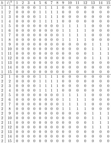
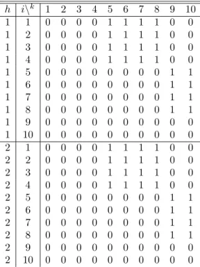
j = 1, 2, . . . , 10) and precedence relations between the welding operations are given in the following table.

Table 4.1: Precedence matrix for Example 1

h i\k ₁ _{2 3} _{4 5} _{6 7} _{8 9} _{10 11 12 13 14 15} 1 1 0 0 0 0 1 1 1 1 0 0 0 0 0 0 0 1 2 0 0 0 0 1 1 1 1 0 0 0 0 0 0 0 1 3 0 0 0 0 1 1 1 1 0 0 0 0 0 0 0 1 4 0 0 0 0 1 1 1 1 0 0 0 0 0 0 0 1 5 0 0 0 0 0 0 0 0 1 1 1 1 0 0 0 1 6 0 0 0 0 0 0 0 0 1 1 1 1 0 0 0 1 7 0 0 0 0 0 0 0 0 1 1 1 1 0 0 0 1 8 0 0 0 0 0 0 0 0 1 1 1 1 0 0 0 1 9 0 0 0 0 0 0 0 0 0 0 0 0 1 1 1 1 10 0 0 0 0 0 0 0 0 0 0 0 0 1 1 1 1 11 0 0 0 0 0 0 0 0 0 0 0 0 1 1 1 1 12 0 0 0 0 0 0 0 0 0 0 0 0 1 1 1 1 13 0 0 0 0 0 0 0 0 0 0 0 0 0 0 0 1 14 0 0 0 0 0 0 0 0 0 0 0 0 0 0 0 1 15 0 0 0 0 0 0 0 0 0 0 0 0 0 0 0 2 1 0 0 0 0 1 1 1 1 0 0 0 0 0 0 0 2 2 0 0 0 0 1 1 1 1 0 0 0 0 0 0 0 2 3 0 0 0 0 1 1 1 1 0 0 0 0 0 0 0 2 4 0 0 0 0 1 1 1 1 0 0 0 0 0 0 0 2 5 0 0 0 0 0 0 0 0 1 1 1 1 0 0 0 2 6 0 0 0 0 0 0 0 0 1 1 1 1 0 0 0 2 7 0 0 0 0 0 0 0 0 1 1 1 1 0 0 0 2 8 0 0 0 0 0 0 0 0 1 1 1 1 0 0 0 2 9 0 0 0 0 0 0 0 0 0 0 0 0 1 1 1 2 10 0 0 0 0 0 0 0 0 0 0 0 0 1 1 1 2 11 0 0 0 0 0 0 0 0 0 0 0 0 1 1 1 2 12 0 0 0 0 0 0 0 0 0 0 0 0 1 1 1 2 13 0 0 0 0 0 0 0 0 0 0 0 0 0 0 0 2 14 0 0 0 0 0 0 0 0 0 0 0 0 0 0 0 2 15 0 0 0 0 0 0 0 0 0 0 0 0 0 0 0

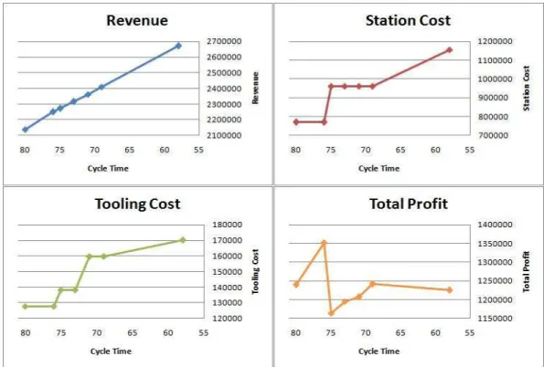
When we solve Example 1 with Algorithm 1, we get different solutions and objective function values corresponding to different cycle times. Figure 4.1 shows the values for the objective function terms and the objective function value as Total Profit for the corresponding cycle times.

As seen in Figure 4.1, revenue, which is the sum of the profits that each product contributes, strictly increases as the cycle times decrease until to γL h

(35)

CHAPTER 4. PROPOSED HEURISTIC ALGORITHM ₂₆

Figure 4.1: Cost and Profit Values for Example 1

values. Station cost is a nondecreasing function as long as the cycle times decrease because lower cycle times require a larger number of stations and it exhibits a stepping structure due to the breakpoints that correspond to particular cycle times.

After giving an insight about the solution of our problem and the nonlinearity of our objective function, we now present our heuristic algorithm that we use for finding initial solutions.

4.1 Heuristic For Finding Feasible Solutions

The heuristic that we introduce in this section consists of several major iterations. The only difference between these iterations are the values of parameter γU

h, the

upper bound on the cycle time for model h, h ∈ G. Using different γU

h values at

(36)

we start with creating a list I of unassigned operations, which initially includes all operations and becomes empty when all of the operations are allocated to the stations. Then, by using predecessor matrix P , for each operation Ohi we create

pred(h, i), a list that includes all predecessor operations of Ohi. In the further

steps of each iteration, while allocating an operation to a station, we need to use the original pred(h, i) lists to ensure that the allocation satisfies precedence constraints, but we also need to update these lists whenever an operation is allocated to a station. Therefore, for each Ohi, we create another predecessor

list dpred(h, i), which is initially a copy of pred(h, i) but is subject to changes in the further steps. The reason for keeping dynamic dpred(h, i) lists is that an operation becomes assignable when its dpred(h, i) list is empty. While assigning the operations to the stations, for each station, we need to keep information about the total time spent and total number of spots performed for a particular model in order to ensure that cycle time and tool life constraints remain satisfied. Therefore, we use loadhj and spothj, which keep the necessary information about

the total time spent and total number of spots performed for a particular model in each station and which are initially equal to τj and 0, respectively.

After these initializations, we start allocating the welding operations to sta-tions. At each step, we allocate only one operation to a station. Therefore, we performPg_h=1nh steps until there is no operation left to allocate, in other words,

I = Ø. At each step, we choose to allocate the operation Ohi with the largest

operation time and whose predecessor operations have all been allocated before. Our selection rule resembles using Longest Processing Time (LPT) rule, which is one of the most popular techniques used in bin packing problems. By allocating the operation with the largest processing time, we aim to have a solution with as few stations as possible, in other words, with as low investment costs as possible. We allocate such a candidate operation to the station with minimum possible index, while ensuring the feasibility of four important constraints. Firstly, the candidate operation should be assignable to that station. Secondly, after allocat-ing the candidate operation, the cycle time for that particular model should not be exceeded. Thirdly, we check if each predecessor operation of the candidate operation has been assigned to the same or to a preceding station. Finally, we

(37)

CHAPTER 4. PROPOSED HEURISTIC ALGORITHM ₂₈

ensure that after allocating the candidate operation, the total number of spots that will be performed at that station between two breaks will not exceed the life of the welding tool at the same station. Once we allocate an operation to a station, we remove it from I, the list of unassigned operations. We update loadhj and spothj for the station that the operation is allocated and remove the

operation from the predecessor lists dpred(h, i) of those other operations for which the allocated operation is a predecessor operation. When the allocation of all op-erations is complete, we calculate objective function value for the corresponding solution.

As mentioned before, our heuristic consists of several major iterations. We start the first major iteration with_bγU

h = γhU values for each h ∈ G. At the end of

each major iteration, we obtain cycle time (fh) values and start the next major

iteration with bγU

h = fh− 1. This setting provides us to obtain different solutions

from each major iteration and we continue this process until _bγU h < γ

L

h for each

h ∈ G. The reason behind this stopping criterion is that achieving a cycle time fh lower than γhL for any model does not contribute any additional profit and

therefore the objective function value does not increase.

In Example 1 that was presented at the beginning of this chapter, the largest objective function value corresponds to the solution in which fh = γh for both

models. But since all objective function terms depend on the values of cycle times, this may not always be the case. In other words, we may obtain larger objective function values with arbitrary cycle times. The following example shows the importance of why we perform a search for different solutions corresponding to different cycle time values over the intervals [γL

h, γhU] for h ∈ G.

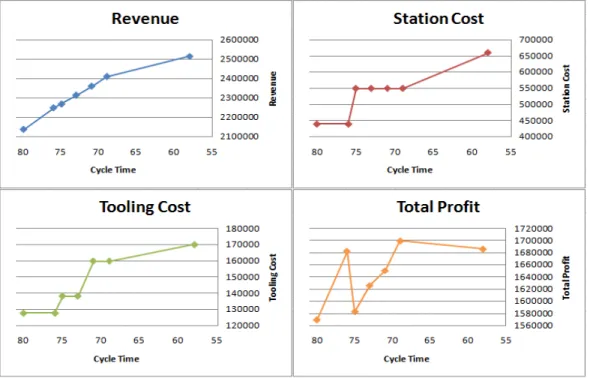
Example 2: Suppose that the company in Example 1 can not sell cars more than the amount that can be produced when the cycle time is 65 seconds instead of 60 seconds for both models (γL

h = 65 for h = 1, 2). Furthermore, the cost of

setting up one station in the assembly line is decreased to $110000 (Vj = 110000

for j = 1, 2, . . . , 10) instead of $192500 in the previous example. All the data provided in Example 1 except these two remain the same. For Example 2, Figure 4.2 shows the values for the objective function terms and the objective function

(38)

Algorithm 1: Heuristic for finding initial feasible solutions

Input: m ∈ IN, g ∈ IN, nh for h = 1, . . . , g, A, P, Whifor h = 1, . . . , g,

i= 1, . . . , nh, Bj and τj for j = 1, . . . , m, γh, γU_h and θh for h = 1, . . . , g.

Output: S, a set of feasible solution(s) begin initialize bγU h = γhU ∀h ∈ G S= Ø while ∃_bγU h such that bγhU ≥ γhL do

Create list I that contains all operations Ohi, h = 1, . . . , g, i = 1, . . . , nh

Create predecessor list pred(h, i) for each Ohi, h ∈ G, i ∈ Nh from P

initialize d

pred(h, i) = pred(h, i), loadhj= τj, spothj = 0 for all h = 1, . . . , g,

i= 1, . . . , nh, j= 1, . . . , m

while I 6= Ø do

Find an operation Ohi∈ I with dpred(h, i) = Ø and maximum thi

Assign Ohi to station Sj with minimum possible index such that

ahij = 1

loadhi + thi ≤ γhU

phik·Pj_l=1xhil+ (1 − phik) ≥ xhkj for each k ∈ pred(h, i) 6300·ψh

max{maxk∈M \j{loadhk},loadhj+thi} · (spothj+ Whi)

+ X

¯ h∈G\h

6300·ψ¯h

maxk∈M{load¯hk} · spot¯hj ≤ Bj

loadhj = loadhj+ thi

spothj= spothj+ Whi

I = I \ {Ohi}

d

pred(c, d) = dpred(c, d) \ {Ohi} for all Ocd∈ I

Let y be the corresponding solution

Find ϕy, the corresponding objective function value

S = S ∪ y

fh ← maxj∈M{loadhj} ∀h ∈ G

bγU

h ← fh− 1 ∀h ∈ G

(39)

CHAPTER 4. PROPOSED HEURISTIC ALGORITHM ₃₀

value as Total Profit for the corresponding cycle times.

Figure 4.2: Cost and Profit Values for Example 2

The two different Total Profit value patterns in Figure 4.1 and Figure 4.2 show that our problem is difficult in the sense that Total Profit is a ‘very nonlinear function’ according to the DICOPT solutions manual. Also, Figure 4.2 clearly shows that there may be multiple peak points of Total Profit function, which means that the global optimum for the objective function value may correspond to particular cycle times in the intervals [γL

h, γhU] for h ∈ G and even for the instances

of NLMIP that can be solved by DICOPT, there is the fact that DICOPT may get stuck in one of the local optima. Therefore, we perform a search for alternative solutions corresponding to different cycle time values over the intervals [γL

h, γ U h]

for h ∈ G. In addition to these facts, we still do not know whether we find the best solution achievable in terms of the objective function value. Hence, in the following section of our study, we will try to strengthen our search methods in order to find better solutions than the ones that we can find with Algorithm 1.

(40)

4.2 Improvement Algorithm

Algorithm 1 presented in Section 4.1 does not necessarily give an optimal alloca-tion of operaalloca-tions in terms of the objective funcalloca-tion value of MIP. In other words, there may be a better allocation of operations that corresponds to cycle times different than the ones that correspond to a solution found by Algorithm 1.

As previously defined, let y ∈ S be a feasible solution that is found by Algo-rithm 1 to our problem. Let my be the number of stations used in the assembly

line in the feasible solution y. As long as the cycle times are larger than the corresponding γL

h values, achieving lower cycle times with less than or equal to

my stations increases the revenue and so the Total Profit, which we aim to

max-imize. Hence, in this section, we present the following problem, in which we use a surrogate objective function to minimize the cycle time of each model to be produced in addition to the overall cycle time denoted by MaxCycleTime.

Minimize MaxCycleTime + g X h=1 fh− γhL Subject to MaxCycleTime ≥ fh ∀h Constraint (2.2) (SP) m X j=1 σj ≤ my Constraints (3.9)-(3.11), (3.13), (3.14) Constraints (2.4)-(2.6) Bj ≥ g X h=1 6300 · ψh · ( nh X i=1 Whi· ehij) ∀j MaxCycleTime ≥ 0, fh, ωh ≥ 0 ∀h, ehij ≥ 0, xhij ∈ {0, 1} ∀h, i ∈ Nh, j, σj ∈ {0, 1} ∀j

In order to achieve better allocations of operations in terms of the objective function value, we reduce our problem to SP. The optimal allocation to SP is still a feasible solution for MIP that is presented in Chapter 3 as shown in the following lemma.

(41)

CHAPTER 4. PROPOSED HEURISTIC ALGORITHM ₃₂

Lemma: Let ¯xbe an optimal solution to SP, then ¯xis a feasible solution to MIP. Proof: In SP, we omit constraints (3.1)-(3.8), (3.15)-(3.17), (3.19)-(3.21), (3.23), (2.8) and (3.24), which are present in MIP. We need constraints (3.1)-(3.8) for linearization of the objective function of NLMIP. Since our objective in SP is different from MIP, omitting these constraints does not affect the feasibility of ¯

x to MIP. We use constraints (3.15)-(3.17), (3.19)-(3.21) and (3.23) in MIP for linearization of constraint (2.7) in NLMIP. Together with constraints (2.8) and (3.24), these constraints ensure that the remaining number of spot welds that a welding tool in station j can perform after tool change time period q is greater than or equal to the number of spot welds it has to perform until the next tool change time period. In other words, we need these constraints to determine the values of zjq variables, which are necessary for calculation of tooling costs in the

objective function. Again, since we have a different objective function and zjq

values are necessary for calculation of tooling costs, omitting constraints (3.15)-(3.17), (3.19)-(3.21), (3.23), (2.8) and (3.24) does not affect the feasibility of ¯xto MIP. 2

Let y ∈ S be a feasible solution that is found by Algorithm 1 to our problem and let my be the number of stations used in the assembly line in the feasible

solution y. We first run SP for my − 1 stations with the same upper bound and

other parameters used in Algorithm 1 that result in the feasible solution y. If the same cycle times in the feasible solution y can not be met by using less number of stations, we run SP again for my stations to improve the cycle times and so

the Total Profit that we want to maximize in the original problem.

Let y ∈ S be a feasible solution that is found by Algorithm 1 to our problem and let ¯y be an optimal SP solution using the same parameters that result in the feasible solution y in Algorithm 1. Let ϕy and ϕy¯ be the objective function

values that correspond to y and ¯y, respectively. Algorithm 2 is a combination of Algorithm 1 and SP.

As mentioned in the previous chapter of our study, the difficulty of our problem results from the fact that our objective function is very nonlinear. In the following example, we will see how DICOPT fails to find the optimal solution and how we

(42)

Algorithm 2: Algorithm for improving heuristic solutions

Input: m ∈ IN, g ∈ IN, nh for h = 1, . . . , g, A, P, Whifor h = 1, . . . , g,

i= 1, . . . , nh, Bj and τj for j = 1, . . . , m, γh, γUh and θh for h = 1, . . . , g.

Output: Best solution begin initialize bγU h = γhU ∀h ∈ G S= Ø, ¯S = Ø while ∃_bγU h such that bγhU ≥ γhL do

Create list I that contains all operations Ohi, h = 1, . . . , g, i = 1, . . . , nh

Create predecessor list pred(h, i) for each Ohi, h ∈ G, i ∈ Nh from P

initialize d

pred(h, i) = pred(h, i), loadhj= τj, spothj = 0 for all h = 1, . . . , g,

i= 1, . . . , nh, j= 1, . . . , m

while I 6= Ø do

Find an operation Ohi∈ I with dpred(h, i) = Ø and maximum thi

Assign Ohi to station Sj with minimum possible index such that

ahij = 1

loadhi + thi ≤ γhU

phik·Pj_l=1xhil+ (1 − phik) ≥ xhkj for each k ∈ pred(h, i) 6300·ψh

max{maxk∈M \j{loadhk},loadhj+thi} · (spothj+ Whi)

+ X

¯ h∈G\h

6300·ψ¯h

maxk∈M{load¯hk} · spot¯hj ≤ Bj

loadhj = loadhj+ thi

spothj= spothj+ Whi

I = I \ {Ohi}

d

pred(c, d) = dpred(c, d) \ {Ohi} for all Ocd∈ I

Let y be the corresponding feasible solution S = S ∪ y

Solve the SP model with the same parameters and find ¯y, the corresponding SP solution ¯ S = ¯S∪ ¯y fh ← maxj∈M{loadhj} ∀h ∈ G bγU h ← fh− 1 ∀h ∈ G

Find ϕy and ϕy¯ for each y ∈ S and ¯y∈ ¯S

Best← argmax_y∈S,¯_{y∈ ¯}_S{max{maxy∈Sϕy,maxy∈ ¯¯ Sϕy¯}}

(43)

CHAPTER 4. PROPOSED HEURISTIC ALGORITHM ₃₄

improve our heuristic results by adding the surrogate problem.

Example 3: Suppose that the company in Example 1 has an available space in their production area only for four stations (m = 4). Suppose further that both models require 10 spot welding operations (nh = 10 for h = 1, 2) and the

number of spot welds required to perform these operations are 10, 8, 8, 7, 10, 9, 8, 7, 10 and 9, respectively. Except precedence relations, all the data provided in Example 1 remain the same. Precedence relations for operations are given in Table 4.2.

Table 4.2: Precedence matrix for Example 3

h i\k ₁ _{2 3} _{4 5} _{6 7} _{8 9} ₁₀ 1 1 0 0 0 0 1 1 1 1 0 0 1 2 0 0 0 0 1 1 1 1 0 0 1 3 0 0 0 0 1 1 1 1 0 0 1 4 0 0 0 0 1 1 1 1 0 0 1 5 0 0 0 0 0 0 0 0 1 1 1 6 0 0 0 0 0 0 0 0 1 1 1 7 0 0 0 0 0 0 0 0 1 1 1 8 0 0 0 0 0 0 0 0 1 1 1 9 0 0 0 0 0 0 0 0 0 0 1 10 0 0 0 0 0 0 0 0 0 0 2 1 0 0 0 0 1 1 1 1 0 0 2 2 0 0 0 0 1 1 1 1 0 0 2 3 0 0 0 0 1 1 1 1 0 0 2 4 0 0 0 0 1 1 1 1 0 0 2 5 0 0 0 0 0 0 0 0 1 1 2 6 0 0 0 0 0 0 0 0 1 1 2 7 0 0 0 0 0 0 0 0 1 1 2 8 0 0 0 0 0 0 0 0 1 1 2 9 0 0 0 0 0 0 0 0 0 0 2 10 0 0 0 0 0 0 0 0 0 0

In this example, the best objective function value that is achievable by Al-gorithm 1 is 1640022 and in this solution, the number of stations used in the assembly line is equal to 3 and cycle times for both models are equal to 73. How-ever, when we run SP, we see that with 3 stations, a cycle time of 69 is achievable for both models. Such a decrease in the cycle time results in more production and so in more revenue. Hence, the best objective value achievable increases to 1735082 by Algorithm 2. Furthermore, the best solution found for this instance by DICOPT has an objective function value of 1702947, which means that DICOPT

(44)

got stuck in one of the local optima of the objective function. Moreover, this relatively small instance of our problem can be solved to optimality by CPLEX in approximately 20 minutes and the optimal value is the same with the one that we find by Algorithm 2. But for this instance, Algorithm 2 finds the optimal solution just in a few seconds.

In this chapter, we have given our proposed heuristic algorithm together with some examples and numerical results. In the next chapter, we will see an overview of the implementation of our tool change decisions to a real-life assembly line problem. In Chapter 6, we will test the performance of our heuristic on some instances of our problem and compare the performances of our heuristic and DICOPT and CPLEX solvers.

(45)

Chapter 5 Implementation

In this chapter, we will give some details about the tool change decision policy that we proposed to solve the real-life assembly line problem that we faced in the project that we had formerly conducted at one of the leading automotive companies in Turkey. As mentioned before, while defining our problem and con-straints in our study, we were inspired by this project. Our aim in the project was to increase the efficiency of an assembly line that performed spot welding op-erations and produced body components for different models of cars. The most important problem of the assembly line was that some tool changes coincided to the times when the assembly line was supposed to be operating. Therefore, in order to perform tool changes, the assembly line was stopped and this resulted in loss of production. In their previous assembly line balancing problems, the com-pany has allocated almost 10% of their available capacity to the line stoppages due to the tool changes. To eliminate such tool change related line stoppages, we developed a decision support system that indicated at which break each of the welding tools in the assembly line should be replaced with a new one. All the relevant information about operation allocations, number of spot welds that each tool must perform and cycle times for each model was provided to us by the company. However, since the assembly line was operating for a long time, we did not have a chance to revise the allocation of welding operations to the stations because it would take a long time to recode the robot operations and

(46)

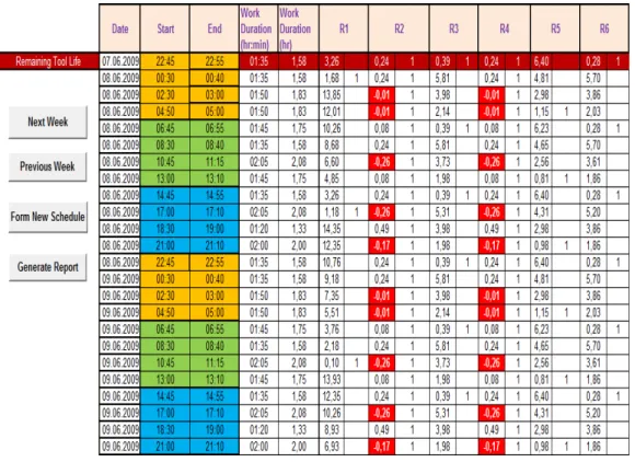
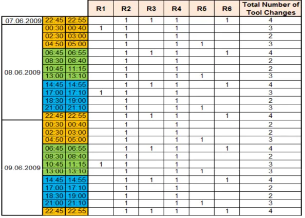
movements and to perform production simulation studies. Therefore, we were able to apply the results of our tool change analysis only to the current system, without changing any operation allocation. Figure 5.1 is a screenshot of one of the modules that we had in our decision support system.

Figure 5.1: Tool change schedules for spot welding tools

Figure 5.1 shows a part of a weekly tool change schedule for spot welding tools. The four buttons on the left are used for returning back to the tool change schedule of the previous week, advancing to the next production week and forming the tool change schedule and generating a tool change report. The dates and the starting and ending hours of each break are given. The work duration column shows the production time between the current break and the next break. R1, R2, R3, R4, R5 and R6 represent the spot welding tools at six different stations. Under these columns, the remaining life of welding tools after each break is given. If the number ’1’ occurs in any cell of these columns, it means that the welding tool has to be changed with a new one at the corresponding break because the remaining life of the tool is not enough for that tool to be used for production

(47)

CHAPTER 5. IMPLEMENTATION ₃₈

until the next break.

If the remaining life of a tool after a particular break is negative and hence the corresponding cell is highlighted (i.e., filled in red), it means that the life of such a tool has expired at some time before the break. Although the tool change decisions are made to eliminate such occurrences and hence tool change related line stoppages, it did not work for all the spot welding tools in the current sys-tem. This might occur for two reasons. In initial allocation of the operations, there might be some spot welding tools with a very frequent usage such that the tool life might be shorter than the available time period. Another reason is that our decision support system uses real time data and once it is executed, it obtains the current time and the remaining number of spot welds that each tool can perform from Welding Management System (WMS), version 2.94, which is a software developed for welding operations by Gf Welding S.p.A. company. Therefore, there might be some deviation between the actual number of compo-nents being produced and the expected demand information that we have used in our formulation due to the unexpected events leading to line stoppages such as the tips of the welding tools may cling on a part during a welding operation, the grippers used for transportation of parts through the assembly line may not close properly or the censors may not recognize or may miscognize a part. For example, although the welding tools R2 and R4 are changed at every break, they still sometimes cause the assembly line to stop between two particular breaks. The reason for such stoppages was that the number of spots that the welding tools R2 and R4 had to perform between two particular breaks as a result of the predetermined operation allocations sometimes exceeded their tool lives in terms of the total number of spot welds that they can perform. Therefore, it can be derived that tool change related stoppages in assembly lines cause from alloca-tion of operaalloca-tions which are determined without considering the limited lives of tools that are used for production. Hence, this is the reason why we determine operation allocations and tool change decisions jointly in our study.

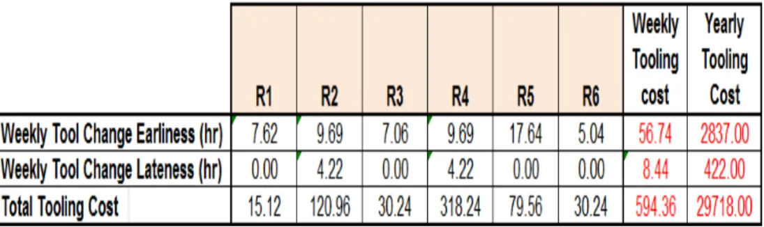
Another useful property of our decision support system is that one can see the corresponding tooling cost that is incurred for particular tool change schedules. Figure 5.2 shows the weekly and yearly tooling costs for a particular tool change