Modelling and control of a wind energy conversion system

Modelling and control of a wind energy conversion system

BEHCET M. SARIBATIRt and MESUT E. SEZER:/:

The dynamical model of a novel low power wind energy conversion system consisting of a' wind turbine, an induction generator, a PWM a.c. inverter and a d.c. battery group is obtained. A feedback control law is developed to provide optimum power conversion and arbitrarily fast responses at steady-state. The feedback does not require measurement of the wind speed and therefore is suitable for real applications. The stability of the closed-loop system is analysed using a Liapunov-type practical stability criterion, and it is shown that the system remains stable for wind speed variations that are not both large and fast at the same time. Digital computer simulation studies on a I kVA test system verify the theoretical results.

1. Introduction

The oil crisis of the early 1970s led to an increasing emphasis on producing electrical energy from other sources. Of these, wind energy seems to be a promising alternative to oil, mainly because it does not cause environmental contamination, and at most sites its seasonal availability shows a good correlation with the seasonal demand for energy. Because of these advantages, wind energy conversion systems are already being used in several applications. However, since wind is not a reliable source of energy, in critical applications wind energy conversion systems are usually backed up with other energy sources such as diesel engines, solar systems, or d.c. battery groups (Akerlund 1982, Tsitsovits and Fresis 1983).

In low power applications, as in telecommunication and radiolink systems, d.c. battery groups provide sufficient back up. In such systems, normally the wind power is used both to supply the load and to charge the batteries, but when the wind power is not sufficient, the load is supplied by the battery. The d.c. voltage required to charge the batteries is usually obtained by rectifying the output of an a.c. generator, which is less expensive, and needs less maintenance than a d.c. generator.

At present, the general trend is to use an a.c. synchronous generator with a diode bridge connected to its stator, where the amount of generation is controlled by varying the field excitation of the generator using a d.c. chopper. A major drawback of such a configuration is that, because of the necessity for operating the generator at different frequencies depending on the wind speed, at low frequencies the magnetic flux density required to obtain the desired d.c. voltage becomes excessively high. This causes saturation of the magnetic parts of the machine, resulting in a considerable reduction in efficiency of the system. Although this can be avoided to some extent by using specially designed machines such as air-cored generators (Eriksson and Ottosson 1983), such special designs increase the cost of the system and introduce difficulties in replacement of the generator. A second disadvantage of using a synchronous generator shows itself in meeting the optimum power conversion

Received 13 July 1986.

t

Department of Electricaland Electronics Engineering, Middle East Technical University, Ankara, Turkey.

328 B. M. Saribatir and M. E. Sezer

condition, which is the main objective of a wind energy conversion system. To optimize the generated power, the speed of the machine should be kept at a certain proportion of the wind speed. This can only be achieved either by measuring the wind speed, which is a difficult task, or by employing a kind of adaptive control mechanism, which again requires complicated measurements and on-line computations (Eriksson and Ottosson 1983). Finally, since the power flow through the diode bridge is unidirectional, the synchronous machine cannot be operated as a motor when required. This necessitates the use of a complicated turbine blade structure to regulate the response of the system, especially at start-up.

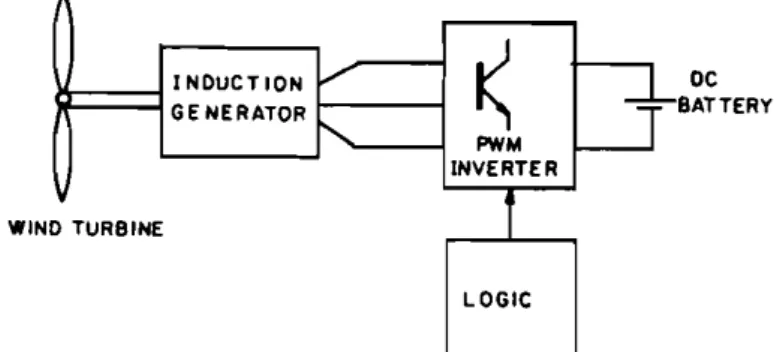
An alternative to using a synchronous generator as the main energy conversion device is to employ an induction generator. Theoretically, the speed of an induction generator can be varied over a wide range to provide maximum power conversion at various wind speeds. The main objective of our paper is to investigate how this advantage of the induction generator can be exploited. For this, we consider the configuration shown in Fig. I, which consists of a wind turbine, an ordinary squirrel-cage induction machine, a PWM inverter, and a d.c. battery group. In this set-up, since all the reactive power required by the induction machine is supplied by the inverter, there is no danger of losing the generator excitation, which may occur when the machine is excited by shunt capacitors as in many other wind energy conversion systems. The amount of d.c. generation is controlled by the frequency and magnitude of the fundamental output voltage of the inverter. By changing the frequency and the magnitude of the output voltage proportionally using a commercial motor control chip specially designed for this purpose (Starr and van Loon 1980), the generator is prevented from being driven into saturation. This eliminates the need for a specially designed machine. X::==lINDUCTlDN JI GENERATOR

1---.,

WIND TURBINE

~

PWM INVERTER LOGIC

Figure I. Wind energy conversion system employing an inverter-fed induction generator. The outline of the paper is as follows. In § 2 we explain briefly the operation of various parts of the system, and obtain an approximate dynamical model based on some mild simplifying assumptions. Using this model, we derive a simple feedback control rule in § 3, which guarantees maximum power conversion in the steady-state. The feedback control requires only the measurement of the turbine shaft speed, and is therefore extremely easy to implement in a real application. In this section, we also show that the speed of response of the system can be adjusted as desired by an additional feedback from the acceleration of the shaft. In § 4, we investigate the stability of the closed-loop system using a Liapunov-type practical stability criterion. We show that, with the wind speed represented as a perturbation superimposed on a

nominal constant value, the system remains practically stable in a region about the equilibrium corresponding to the nominal wind speed, unless the variations in the wind speed are not both large and fast. We also derive upper bounds for the magnitude and rate of wind speed variations for practical stability of the system. Finally, in § 5, we briefly summarize the results of a digital computer simulation of a I kva test system both for deterministic wind speed variations, to verify the results of our theoretical analysis, and also for stochastic variations, to get a better idea about the behaviour of the system under more realistic conditions.

2. Dynamical model of the system 2.1. PWM inverter

The d.c. generation phenomenon in an inverter-fed induction machine has long been observed in motor control applications (Novotny et al. 1977, Melkebeek and Novotny 1983), but has never been used for the purpose of generating d.c. power by an induction machine driven by an external source such as a wind turbine.

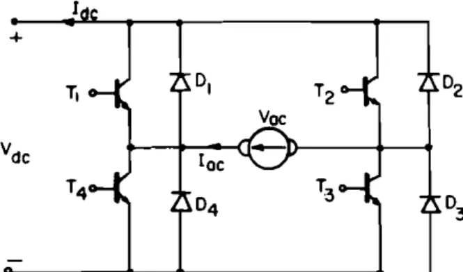
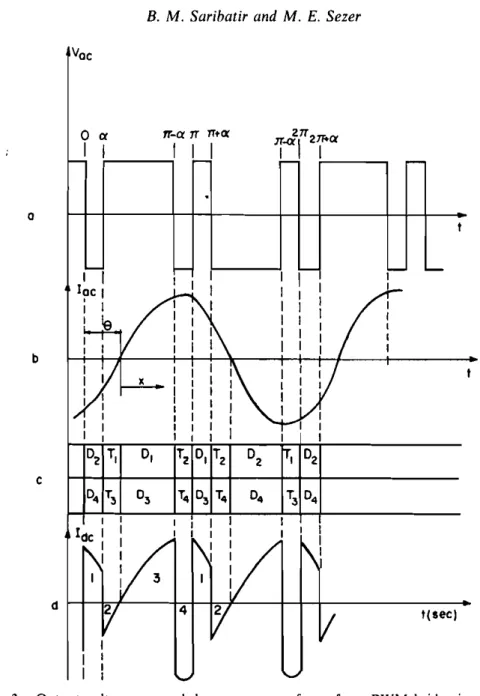
The basic configuration of a PWM inverter feeding an induction machine is shown in Fig. 2. For a simple PWM voltage waveform 1';..,. and a sinusoidal machine current Ia.'. as shown in Fig. 3(a) and Fig. 3(b), the d.c. current through the constant voltage source, corresponding to a conduction sequence of the transistors and the freewheel-ing diodes shown in Fig. 3(c), has the waveform in Fig. 3(d). By a simple analysis of the voltage and current waveforms in Fig. 3, the amount of generated d.c. power can be computed as (Saribatir 1985)

r,

= V.I,

cos

e

(I)

where

V.

and

I,

are the r.m.s. fundamental stator voltage and current and

e

is the phase angle between the two. In practice, a high performance PWM inverter designed for motor control applications has a switching frequency well above the fundamental frequency, so that the machine current can be assumed to be sinusoidal for all practical purposes. Thus, (I) is indeed a valid expression for the generated power.

2.2. Induction generator

When the system has a sufficiently large inertia so that the variations in the shaft speed are not fast compared to the electrical time constants of the machine, the

steady-+

T1

°2

Vdc T4

°3

Figure 2. Transistorized single phase bridge inverter.

330 B. M. Saribatir and M. E. Sezer V_oc o

o

Cl IT-aIT 1TtOC

_I ;..-'

---i'

U

ZIT IT.()(

I

Z1t+Cl 1- ;-,_ _--, b c

J{

I:I

f--L-

!:

I I \I -W

.r

I : I I : I I I I I I I : : : I I I I I I I I I I

I~i~:

I 11\:

Vi

1

I I :5 I I

L

V

4

l!

v

!(sec)

Figure 3. Output voltage, a.c. and d.c. current waveforms for a PWM bridge inverter with sinusoidal output current.

state approximate equivalent circuit shown in Fig. 4 provides an adequate model for the induction generator for a sinusoidal machine current. Using (I) and the equivalent circuit in Fig. 4, the d.c. power generated by a three-phase induction machine can be approximated, for small values of the slip s,as

(2) where r, is the rotor resistance. The minus sign is introduced to obtain a positive

quantity for the power as the slip takes negative values.

It is observed from (2) that the same power is generated for infinitely many combinations of the stator voltage

V,

and the slip s. It can easily be shown that to maximize the generator efficiency, the slip should be kept as small as possible (which is also required for the expression in (2) to be a better approximation of the actual

rr

Figure4. Steady-state equivalent circuit of an induction generator.

generated power). On the other hand, increasing the stator voltage beyond a certain limit results in saturation of the machine. A reasonable compromise is to keep the stator voltage-to-frequency ratio at the rated voltage-to-frequency ratio of the machine. Thus, the stator voltage at a given frequency j, is chosen as

v,

= (Vo/fo)!. (3)

where V_oand fo are rated stator voltage and frequency of the machine.

Finally, for small values of the slip, the stator frequency can be approximated by

f,=

Nw (4)

where w is the turbine shaft speed and N is a constant that takes into account the

number of poles and the mechanical coupling ratio of the machine. Thus, substituting (3) and (4) into (I), the expression for the generated power becomes

(5) 2.3. The wind power and turbine characteristics

In this paper, the amount of wind power which is converted into mechanical power by the turbine will be given by the following relation, which has already been used in some other works (Anderson and Bose 1983),

(6)

where K is a constant, v is the wind speed and c is the turbine efficiency coefficient. This coefficient is a function of the tip speed ratio, defined as the ratio of the speed of the tip of the blades to the wind speed as

,1.=Rw]»

(7)

where R is the radius of the turbine. The efficiency coefficient c_pis usually represented graphically, but can be approximated analytically as (Anderson and Bose, 1983)

Cp(A)

=

a(b/,1.- 1)exp (- c/).) (8)

where a, band c are parameters related to the mechanical construction of blades. The optimal value of the tip speed ratio, at which the efficiency coefficient cp attains its maximum, can be computed from (8) as

,1.0= cbj(b

+

c)

(9)

Thus, in order to extract maximum power from the wind at any speed v,the shaft speed should be kept at a value w

=

Aov/R if possible.

332 B.M. Saribalir and M. E. Sezer 2.4. Overall dynamical model

Since the viscous friction torque is small compared to the generated torque and the variations in the shaft speed are not fast, the effects of friction and the stiffness of the shaft on the dynamic behaviour of the system can be neglected. Thus, assuming that all the net power in the turbine/generator assembly is used to accelerate the shaft,

( 10)

whereJ is the overall inertia of the system. Substituting the expressions for p.and Pw

given in (5) and (6) into (10), a dynamical model of the overall system is obtained as (11)

In(II), we identify wor

A

as the controlled variable (whichever is more convenient for a particular purpose),sas the control input, and v,which does not appear explicitly in (II), but is included implicitly in

A,

as the disturbance.

3. Control structure

The objective of the control is to adjust the slip sin the dynamical model given by (I l] such that the tip speed ratio is regulated at its optimal value .1._{0 ,}Since the system is highly non-linear, regulation of Aagainst arbitrary variations in the wind speed is extremely difficult, if not impossible. However, as the first step of control design, maintaining the optimal tip speed ratio under steady-state operating conditions, i.e. when the wind speed is constant, should be aimed for.

At steady-state, IV= 0, and (II) reduces to

(12) from which we obtain a linear relation between the slip and the shaft speed as

(13) where

( 14)

Relation (13) provides a simple feedback law which guarantees optimal steady-state operation. This can better be seen by substituting (13) and (14) into (11), which yields

(15) Indeed, for a constant wind speed

v

=

v"

w

=

Aovc/R is a solution of the differential equation in (15) corresponding to J.

=

J._o.

Itshould be noted that the feedback law in (13) involves only the shaft speed, and is therefore extremely easy to implement. This is probably the greatest advantage of the configuration we consider in this paper over other wind energy conversion systems.

Although the feedback law given by (13) is derived with the objective of keepingJ.

at .1.₀ under steady-state conditions, it also provides some regulation on J. against stepwise changes in the wind speed, as we discuss below.

Let (15) be rewritten as

where

(17)

A plot of f().) is shown in Fig. 5, from which we identify two roots at ),

=

i'l and

). =

A_z

=

A_o.When the wind speed is constant atv

=

v"these roots define two equilibrium points of the system as w

=

w,

=

A,vc/R

and w

=

W_z

=

)'zvc/R. Obviously, w

=

W3

=

0

is a third equilibrium point.

The behaviour of the system for constant wind speed can now be investigated with the help of Fig.5.Suppose that, initially, the tip speed ratio has the value A

=

A;= Rw.to; corresponding to an initial shaft speed w

=

W;.

(a) IfA;>A2 ,thenf(A) <0and w decreases with time, corresponding to a decrease

in A. Eventually, A reaches A2 , and the optimal operating conditions are

recovered.

(b) If )" <A;< )'z,then f(A)> 0, and this time wand A increase with time. Again,

the system comes to a rest when),

=

i'2

=

)'0'

(c) IfA;<AI,thenf().) <0,and w decreases to W3,and the system comes to a stop,

Ol---,~---'Ir_---~

Figure 5, Plot off().) against ).,

This discussion shows that, when the wind speed is constant, and A>)'1 initially, then the feedback law given by (13) brings the system back to the optimal operating point, and thus guarantees a stable operation, However, the dynamical performance of the system may not be satisfactory due to either a very large or very small inertia of the system, This can better be seen by examining (16) more closely, which reveals that, with the wind speed constant, the acceleration of the shaft at any speed is determined completely by the inertia of the turbine, Hence, the feedback in its present form does not provide any improvement in the speed of response of the system, On the other hand, if some information about the rate of change of the shaft speed is included in the feedback law, this information can be used to help the turbine to speed up or to slow down more quickly to keep pace with the wind speed variations. In other words,ifan increase in the shaft speed is detected, which indicates an increase in the wind speed, then, by reducing the generation, more of the wind power can be used to accelerate the shaft faster so that the tip speed ratio does not stray far from the optimal value, In

334 B. M. Saribatir and M. E. Sezer

such a case, the induction machine may even be operated as a motor. This can easily be managed since the power flow through the inverter is bidirectional. Of course, in the reverse situation, when the turbine shows a tendency to slow down as a result of a decrease in the wind speed, then, by increasing the generation, some of the kinetic power of the shaft is transferred to the battery to help the slowing down of the turbine. Simulating the system on a digital computer for several wind speed profiles, it has been observed that the dynamical performance of the system could be changed as desired if the feedback law given by (13) is modified by including a term concerning the acceleration of the shaft as

(18) where k₂is a constant. The form of the additional feedback is no coincidence. Indeed, substituting (18) into (II), the closed-loop model given by (16) is modified into

(19) where

(20) The modified model in (19) has the same form as that in (16), and the equilibrium points of the system under dynamic feedback are the same as before. The only effect of the additional feedback is to change the equivalent inertia of the system. The value of the equivalent inertia can be made arbitrarily small or large by selecting the feedback constantk, appropriately. Thus the speed of response of the system can be changed as desired.

Finally, it should be pointed out that if the friction(D)and stiffness(k)of the shaft are taken into account, then by modifying the feedback law in (18) as

(18') optimum steady-state operation and arbitrary speed of response can be recovered. How-ever, in general, Dand F are sufficiently small and can be omitted in real applications.

4. Stability analysis

Since the dynamical model of the closed-loop system is highly non-linear, it is not possible to obtain an analytical solution of the dynamic system even for simple deterministic variations in the wind speed. Although the analysis of the system for step changes in the wind speed gives an idea about the roles of the critical values )., and )'2' it is of very little practical value because actual wind speed variations are very complicated. Furthermore, since the system does not have an equilibrium point for a varying wind speed, it is also not possible to apply the standard Liapunov method directly. Fortunately, however, a variation of Liapunov's method concerning the stability of solution sets can be used to derive conditions on the wind speed variations that ensure an acceptable behaviour of the resulting solutions. In the following, we first summarize the concept of so-called practical stability (La Salle and Lefschetz 1961, Michel and Miller 1977), and then discuss how this concept can be applied to our system.

Consider a dynamic system represented by

where u

=

u(t) is an external input to the system and x is the state vector. Assume that

the system in (21) possesses a unique solutionx(t, xo, u) for every initial state x(O)= xo,

and every input ubelonging to a certain class 0/1, but the existence of an equilibrium point is not required.

Let .'1'1 and .'1'2 denote two open subsets in the state space, such that

g,

c .'1'2.The system represented by (2\) is said to stable with respect to {g"

S'2}

_{if Xo E'.'I'1 implies} that _{x(t, x o, u) E'.'I'2 for all t}>0 and for all u E'0/1 (Michel and Miller \977). To investigate the stability with respect to {g".'I'2}' we consider a scalar function V(x)

with continuous partial derivatives for all x such that V(xtl

<

V(X2) for all XI E'.'I',

and X2 E' .'1'2 - .'1'1.IfV(x)

<

0 for all x E'

92 -

.'1'1 ,then every solution of (21) starting in the region

g,

remains in .'1'2 (LaSalle and Lefschetz 196\).

To apply the concept of practical stability to the dynamical model given by (19), we first assume that the wind speed is described as

v=vc[I +u(t)] (22)

where V_c is a constant, the nominal value of the wind speed, and u(t) represents the

variations in the wind speed normalized by the nominal value. Then, defining a new variable as x= _(v/vc))'- A₂= [I

+

u(t)]). - A₂= _{(Rw/v c) - )'2} we transform (19) into and choose (23) (24) (25) V(x)= -

fa'

fly

+

A2 )dy

We note that for arbitrary intervals

g,

and .'1'2 on the real line satisfying line satisfying .'1', c

92

= ()., - )'2,00), V(xtl< V(x2 ) for all XI E'.'I', and X2 E'.'I'2 -

g,

as can easily

be verified with the help of Fig. 5. At this point, rather than first fixing .'1', and

92

and then trying to find an upper bound on magnitude of u(t) to satisfy the stability

condition V(x)<0, x E' .'1'2 - g" we aim at determining .'1'1 and .'1'2 such that the stability condition is satisfied with the least restrictive bound on u(t). For this, we

assume that

lu(t)1<e

and compute

V(x)= -(vc/RJeq)f(x

+

_A2)f [(x

+

A2)/(1

+

u)](x

+

A2)2

Now letting

.'1',=(-<5,,<52), .'I'2=(AI-A 2+<53,<54)

where <5j are arbitrary positive numbers satisfying

AI - A

2

+

<53

<

-<51

<

°

<

<52

<

<54

(26)

(27)

(28)

(29)

it can be shown with the help of (27) and Fig. 5 that V(x)

<

°

for all x E' .'1'2 -

g,

provided

336 B.M. Sarihatir and M. E. Sezer

To maximize Emax subject to the inequalities (29) and (30), we choose <5 1

=

<5 2

=

[A2().2 - )'1 - 2j1.)·2!(AI

+

)'2)]

<53

=

Al(A2 - ).tl!()·I

+

A2 )

<54> _{<5 2}

where II is an arbitrary small positive number, which yield Emax

=

[A2(1 - 2j1.) - AI]!(A,

+

A2)

(31)

(32) Using straightforward computations it can be shown that, for a normalized variation in the wind speed bounded by the quantity in (32), the tip speed ratio satisfies

(33) as expected. A more interesting observation is that Ema x given in (32) is the largest possible upper bound on u(t) that can be obtained with no other information on the

nature of the wind speed. Indeed, this bound guarantees practical stability of the system for a step change from

Vmi"

=

vc(1 - Ema x ) to Vma x

=

vc(1

+

Em ax )

However, the ratio

is the maximum allowable per cent step change in a constant wind speed as can easily be verified using the argument in the preceding section.

On the other hand, it is observed from digital computer simulation studies on a test system that larger variations in the wind speed can be tolerated if the variations do not occur too quickly. This observation indicates that the class of tolerable wind speed variations can be enlarged if additional information about the change of wind speed can be made use of in the stability analysis. To investigate this possibility, we define a new state variable

z

as

and transform the model in (19) into

i

=

v(z

+

_A2)[(Z

+

_A2)f(z

+

_{A2)/RJ ,q- li!v}2]

(35)

(36)

(37)

(38a)

(38b) Choosing the same Liapunov function given in (25) but with the argument x replaced by z, and following similar reasoning as for the previous stability analysis, it can be shown that if

then V(z)

<

OforZm - <5 2

<

z

<

z.,

+

<5 1and for z ,

<

Z

<

Z2,where u is an arbitrary small

positive number,

Zm= arg max {(z

+

)'2)f(z

+

A2l),

A, -

A2

< z<0

M = (zm

+

)'2)f(zm

+

)'2) <5 1and _{<5 2}are defined such that

(z

+

A2)f(z

+

)'2)

<

M - j1.

for Zm - <5₂

<

Z

<

Zm

+

<5" and z, and Z2 are defined such that

(38c)

for 0

<

Zt

<

Z

<

Zz.Thus, inequality (37) guarantees practical stability of the model in (36) with respect to

{?"

.'I'z} with?,

=

(zm

+

.5

" z.],

.'I'z

=

(zm - .5z, zz). Expressing the inequality in (36) in a weaker form as

(39) we observe that slowly varying wind speeds are better tolerated. Also, the maximum allowable rate of change in the wind speed can be made arbitrarily large by making the equivalent inertia of the system sufficiently small by increasing the gain of the feedback from the acceleration of the shaft. However, a very small equivalent inertia is not desirable for several practical reasons. Firstly, a small inertia means increased sensitivity to noisy variations in the wind speed. Secondly, it forces the turbine to follow the rapid changes in the wind speed, which requires frequent switching in the mode of operation of the induction machine between generating and motoring. This, however, not only results in a non-uniform power generation, but also increases the losses in the system, causing overheating and reducing the reliability.

S. Digital computer simulation of a 1 kva system

The optimum power transfer criteria stated in the previous sections give an idea about the selection of the feedback parameters. However, since these criteria have been obtained by making some simplifications, before implementing the feedback law in an actual system it is very useful to perform a detailed digital computer simulation of the system to observe its performance in a real environment. For example, the effect of stochastic variations in the wind speed on the operation of the system can easily be simulated for several combinations of the feedback parameters to make a realistic choice. Such a simulation can also be performed many times for different values of the system parameters to determine the sensitivity of the overall system to parameter changes. This is quite important since the stator and rotor resistances of the induction generator vary with temperature.

In this section, we report the results of a digital computer simulation of a I kVA system.

5.1. System parameters

The wind turbine that is supposed to be used in the system has three blades on a vertical axis with a radius of R= \·5 m. The total inertia of the system is about J

=

100 kg m '. The input mechanical power is given by (6) and (8) where K

=

3·95,

a

=

45·85, b

=

4·7 and c

=

14·4, and the optimum tip speed ratio for this particular turbine is computed to be A_o

=

3·55.

The inverter is a fully transistorized three phase PWM inverter whose d.c. terminals are connected to a 48 Vd.c.battery group. The rated fundamental a.c. output

voltage of the inverter is about Vo

=

18 V,.m.s. (line-to-neutral) with a frequency of fo

=

50 Hz. Hence, the output voltage at any frequency f, can be found from (3) as

V,

=

0·36f,.

The induction generator is considered to be a three-phase 1kVA squirrel-cage induction generator whose stator can directly be connected to a 18 VLm.s., 50 Hz source. If the magnetizing branch of the equivalent circuit is omitted, other circuit parameters may be given as rs

=

r,

=

0·05nj<1land x,

=

x,

=

O· 20nj<1l.The constantN which relates the stator frequency to the angular speed of the turbine is taken to be

338 B. M. Saribatir andM. E. Sezer

5.2. Feedhack parameters

With the above choice of the system parameters, the feedback parameter k1can be computed from (14) as k1= 1·95X 10-3s. However, the relation between the slip and

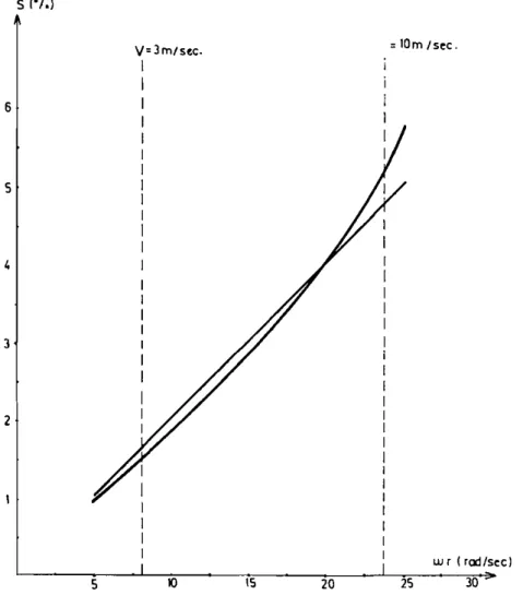
the shaft speed to operate the actual system at the optimal tip speed ratio under constant wind speed is actually a non-linear one as represented by the curve in Fig. 6.

5 ('I.) V=3m/stc. = 10m tsec . J I 6 I I I I J 5 I I I I I I I I I I 3 I I I I 2 I I 5 10 IS 20 25 LlJr ( raj/secJ 30

Figure 6. Slip plotted against turbine speed for optimum wind power input.

A linear approximation to this curve for wind speeds below 10m s -, (at which the rated output power is obtained) has a slope of2·05 x 10-3_{s, which is taken to be the} actual value ofk, in the simulation studies. For this value of k1 , the roots of f().) are computed numerically to be ).,

=

2·06 and)'2= 3·5.Itcan be seen that the second root is approximately equal to the optimum value of the tip speed ratio.

The slight difference between A2 and )'0 obviously results from choosing the velocity feedback gain k, to be slightly different from the value computed from (14).It is appropriate to note at this point that such a different choice may be made intentionally to improve the stability of the system at the expense of optimal operation. Indeed, as can clearly be seen from Fig. 5, choosing a smallerk , raises the

f(J.) curve, resulting in a smaller )., and larger)'2'Obviously, a smallerAI means

mor~

tolerance to wind speed variations, indicating improved stability. However, a value of ,1.2 larger than)'0 means a suboptimal operation at steady-state. Thus, the choice ofk1 provides a compromise between stability and optimality.

The choice of the acceleration feedback gain k2 is not as straightforward as the

choice of kl , and should be based on simulation studies to reach a compromise

between stability, speed of response and smoothness of power generation. In the simulation, three different values of k_{2 ,} namely, k2= 0, k2= 1·5 and k2= 2,

corre-sponding to respective equivalent inertias of Je q= 100kg m", Je q = 43 kg m

2

and Jeq

=

23 kg m', are considered.

5.3. Simulation results

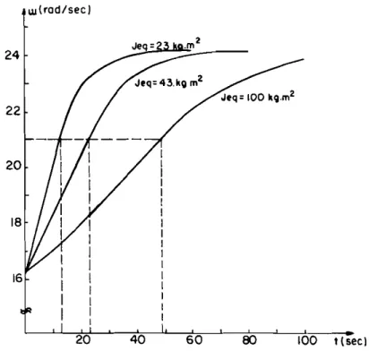
The first simulation is concerned with the response of the system to step variations in the wind speed. Figure 7 shows the shaft speed variations for a step change in the wind speed from an initial value v,

=

7 m s -1 to a final constant value Vf

=

10m s - , for three different values of the equivalent inertia.Itis assumed that prior to the step change in the wind speed, the system is at steady state with an initial shaft speed

w,

= )'2v;/R = 16·3 rad s-'. From Fig.7 it is observed that the systems with

Je q= 43 kg m' and Je q = 23 kg m

2 _{respond approximately two and four times faster}

than the system with Je q= 100 kg m2 (the three systems reach the same shaft speed

of 21 radS-1 at t, = 13 s,t₂= 23 sand t₃= 49 s, respectively). This indicates that the effective time constant of the system is proportional to the equivalent inertia, thus verifying the assertion that the speed of response of the system can be adjusted as desired by varying the value of the feedback parameter k_{2 .} Note that in these

w(rod/sec)

60 00 100 t(sec)

Figure 7. Responseof the systems to a step change in the wind speed for differentvalues of the equivalent inertia.

340 B.M. Saribmir and M. E. Sezer

simulations the final wind speed v(is chosen below the allowable maximum value determined from (34). Indeed, in another simulation it has been observed that for

v(

=

12 m s -1, the shaft speed continuously drops from the initial value to zero

independently of the equivalent inertia, indicating instability.

A second simulation is performed for a deterministic wind speed given as v(t)

=

7

+

3 sin Ft, for which the normalized variations exceed the allowable bound

emu,

=

0,26obtained from (32). In this case, stability of the system should depend

criti-600 Jeq=43k9m2

/

01--_--'--_-'-_----'--_---'-_----'_ _.1...-_-'---_---'---_----'--_----'-_ _ Jeq= 23kgm2 / JeQ=43 kgm2 14 10 u

..

on

....

E >

o

20 40 60 80 I (sec) 100

cally on F and J,q' For J,q = 43 kg m2, the maximum allowable frequency can be

computed with the help of (39) asFmax

=

0'006 rad s -1. Indeed, it is observed that for

F

=

0·005 rad s- I , a value which is very close to the limit value, the system shows a stable operation; while for F

=

0·05 rad s -1, it collapses.

Finally, to observe the system behaviour in a more realistic environment, a third group of simulations has been performed for stochastic wind speed variations which are represented by a gaussian first order autoregressive time series with a mean of 7 m s -1, a standard deviation of 1·05 m s - 1 and an autoregressive time constant of

10 s. The simulation results are shown in Fig. 8, which shows that the shaft speed follows the wind speed variations more closely as the equivalent inertia gets smaller, indicating a faster response. Although at first glance this seems to be a desirable property, an investigation of the output power variations shown in the same figure indicates that it may not be so desirable for the healthy operation of the generator and the inverter. By comparing the plots and computing the total energy pumped into the battery over a fixed period of time, it is concluded thatJ,q

=

43 kg m2

,corresponding

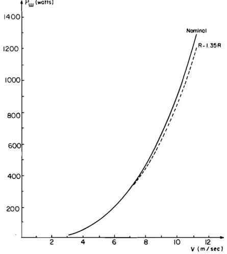
to k₂= 1'5, is a reasonable choice, providing stable operation for a sufficiently large class of wind speed variations without causing too much fluctuation in the generated power. P_w(watts) 1400 Nominal 1200 1000 800 600 400 200 2 8 10 12 V (m/sec)

Figure 9. Input wind power plotted against wind speed for two different values of machine resistance.

342 B. M. Saribatir and M. E. Sezer

5.4. Sensitivity to parameter changes

The parameters of induction generators of the same rating from different manufacturers are different. Hence, the feedback parameters of the control loop have to be adjusted when the generators in the wind energy conversion systems described in this paper are replaced with new ones. This does not cause much trouble since in practice the generators need not be replaced too frequently. However, the parameters of the generators may also change with temperature during operation. The values of the resistances increase as the generator is operated and heated up. This may require continuous adjustment of the parameters to maintain optimal operating conditions at steady-state.

The effect of a change in the rotor resistance on the net power extracted from a steady wind can be examined with the help of Fig. 9, which shows wind power plotted against wind speed for two different values of machine resistances. The values of resistances correspond to the values at 20°C and 110°C. Since there is only a very slight difference between the curves in Fig. 9, we can safely assume that temperature variations do not cause significant deterioration in the performance of the system.

6. Conclusions

In this paper, a novel wind energy conversion system has been introduced. The main features of this system are briefly summarized below.

(a) It is very suitable for small to medium scale electrical power generation for isolated applications such as distant telecommunication and radiolink supplies.

(b)Since the generated power is converted into d.c., no control on the frequency and voltage of the induction machine is required. Such controls, however, can be used to optimize the performance of the system.

(c) The inverter between the generator and the battery group not only facilitates easy control of the stator voltage and frequency, but also provides a bidirectional power flow between the two allowing the induction machine to be operated as a motor if necessary to improve the dynamical performance. Italso eliminates the need for complicated turbine blade structures required to start the system from a standstill.

(d) There is no excitation problem of the induction generator. All the reactive energy is supplied by the inverter.

On the other hand, the main disadvantage of the system is that it requires an inverter for power conversion. Inverters are the most expensive electronic power converters. However, the increased production of high speed bipolar transistors and power FETs in large quantities is continually reducing inverter prices. Nowadays, transistorized inverters with a power rating of 50 kVA are available from the stock of various manufacturers at a reasonable price. Hence, they are very suitable in applications where the rating of the generator is only several horse power. In this - range, the total cost of the power circuitry consisting of a standard induction machine and an inverjer is expected to be less than that of an alternative system consisting of a bridge reciificr,: a d.c. chopper and' a specially designed air-cored' synchronous generator. As a result, induction generators, which are commonly used to generate a.c. power in wind energy conversion systems, also look very suitable for d.e. power generation.

REFERENCES AKERLUND, 1., 1982,Ericsson Rev., 59, 40.

ANDERSON, P. M., and Boss; A., 1983,I.E.E.E. Trans. Power Appar. Syst., 102,3791.

ERIKSSON, M., and O'rrossox,J., 1983,Ericsson Rev.,60,159.

LASALLE,1. P., and LEFSCHETZ, S., 1961,Stability by Liapunou's Direct Method With Applica-tions (New York: Academic Press).

MELKEBEEK,1. A. A., and NOVOTNY, D.

w.,

1983,I.E.E.E. Trans. Power Appar. Syst., 102, 2725. MICHEL, A. N., and MILLER, R.K.,1977,Qualitative Analysis of Large Scale Dynamical Systems

(New York: Academic Press).

NOVOTNY, D.

w.,

GRITTER, D.J.,and STUDTMANN, G. H., 1977,I.E.E.E. Trans. Power Appar. Syst., 96, 1117.

SARIBATIR,B.M., 1985, Modelling and control of a wind energy conversion system consisting of a wind turbine and an inverter-fed induction generator. Ph.D. thesis, Middle East Technical University, Ankara, Turkey.

STARR, B.G., and van LOON, J.C. E, 1980,Electronic Components Appl.,2, 219. TSITSOVITS, A.J.,and FRESIS, L. L., 1983,Proc. lnstn elect. Engrs, Pt A, 587.