REAL-TIME PREDICTION BASED SNOW
AND RAIN ACCUMULATION IN VIRTUAL
ENVIRONMENTS
a thesis submitted to
the graduate school of engineering and science
of b˙ilkent university
in partial fulfillment of the requirements for
the degree of
master of science
in
computer engineering
By
Nail Akıncı
September 2016
REAL-TIME PREDICTION BASED SNOW AND RAIN ACCUMU-LATION IN VIRTUAL ENVIRONMENTS
By Nail Akıncı September 2016
We certify that we have read this thesis and that in our opinion it is fully adequate, in scope and in quality, as a thesis for the degree of Master of Science.
B¨ulent ¨Ozg¨u¸c (Advisor)
Tolga C¸ apın (Co-advisor)
U˘gur G¨ud¨ukbay
Yusuf Sahillio˘glu
Approved for the Graduate School of Engineering and Science:
Levent Onural
ABSTRACT
REAL-TIME PREDICTION BASED SNOW AND RAIN
ACCUMULATION IN VIRTUAL ENVIRONMENTS
Nail Akıncı
M.S. in Computer Engineering Advisor: Prof. Dr. B¨ulent ¨Ozg¨u¸c Co-Advisor: Assoc. Prof. Dr. Tolga C¸ apın
September 2016
Although weather effects have been developed thoroughly in offline renderings, their computational cost exceed current hardware to run them in real-time. Therefore, less expensive methods are developed. Still, in many real-time ap-plications weather conditions are prepared by artists for each environment in-dependently because developers do not want to compromise performance over simulated weather. The main reason of this is current developed algorithms use most of the graphical processing power just for weather effects in a relatively small scale scene. At the end, they become unusable in real scenario, because weather conditions are only one part of the overall system. Therefore, in current approach, all weather conditions are executed based on predictions, where its computational cost is negligible under 0.5 ms on current generation hardware. Predictions are done based on many factors such as orientation, height and position on terrain and global wind and sun direction. Appearance of weather conditions are generated from original textures of the objects then compared and re-adjusted to achieve similar values of real life scanned Bidirectional Reflectance Distribution Function (BRDF) data. All computation is done on Graphics Processing Unit (GPU) to be used with Physically Based Rendering (PBR) approach. Even though all changes are made based on prediction and textures are generated, at the end, results are comparable to weather conditions in real life.
¨
OZET
SANAL ORTAMLARDA GERC
¸ EK ZAMANLI TAHM˙IN
BAZLI KAR VE YA ˘
GMUR B˙IR˙IKMES˙I
Nail Akıncı
Bilgisayar M¨uhendisli˘gi, Y¨uksek Lisans Tez Danı¸smanı: Prof. Dr. B¨ulent ¨Ozg¨u¸c Yardımcı Danı¸sman: Do¸c. Dr. Tolga C¸ apın
Eyl¨ul 2016
C¸ evrimdı¸sı hesaplanan hava durumu efektlerinin olduk¸ca detaylı olarak ara¸stırılmasına ra˘gmen, g¨un¨um¨uz donanımında ger¸cek zamanlı ¸calı¸stırmak m¨umk¨un degil. Bu y¨uzden daha az hesaplamalı y¨ontemler geli¸stirildi. Buna ra˘gmen, ger¸cek zamanlı programlarda hava ko¸sulları, her mekan i¸cin sanat¸cılar tarafından tek tek hazırlanıyor, ¸c¨unk¨u yapımcı ¸sirketler, simulasyon i¸cin eks-tra performans kaybetmek istemiyorlar. Bunun asıl sebebi ise g¨un¨um¨uzdeki al-goritmaların, k¨u¸c¨uk sahneler i¸cin bile hesaplama g¨uc¨un¨un b¨uy¨uk kısmını kul-lanıyor olmalarıdır. Sonu¸c olarak, hesaplamalar gere˘ginden fazla kaynak kul-landı˘gı i¸cin tercih edilmiyorlar. Bu tezde kullanılan y¨ontemde hava ko¸sulları tahmine dayalı hesaplanıyor, bu y¨uzden toplam hesaplama s¨uresi 0.5 milisaniye-den daha az bir seviyede oluyor. Hava durumundan olu¸san birikmelerin tah-mini; sahnedeki objenin oryantasyonu, yery¨uz¨u, y¨ukseklik, pozisyon, g¨une¸s ve r¨uzgarların y¨on¨une g¨ore de˘gi¸siyor. Hava ko¸sullarının etkisi, objelerin orjinal kaplamalarından olu¸sturuluyor ve daha sonra ger¸cek hayattan taranan veri, ˙Iki Y¨onl¨u Yansıma Yayılım Fonksiyonu (˙IYYF) do˘grultusunda kar¸sıla¸stırılıp d¨uzeltiliyor. T¨um hesaplamalar Grafik ˙I¸slem Birimi’nde (GIB) Fiziksel Bazlı G¨orsel Hesaplama (FBGH) y¨ontemi ile kullanılmak ¨uzere i¸sleme sokuluyor. Hava ko¸sulundaki t¨um degi¸simlerin tahmine dayalı olmasına ve objelerin orjinal kapla-malarından olu¸sturulmasına ra˘gmen, sonu¸clar ger¸cek hava ko¸sullarına yakla¸sık bir g¨or¨unt¨u olu¸sturuyor.
Anahtar s¨ozc¨ukler : Hava Durumu Sim¨ulasyonu, Ger¸cek Zamanlı, Birikme, Tah-min Bazlı.
Acknowledgement
First of all, I would like to thank Prof. Dr. B¨ulent ¨Ozg¨u¸c for his guidance and sensibility in my hardest times throughout my master’s program. I am grateful to Assoc. Prof. Dr. Tolga K. C¸ apın for his co-supervision. I would like to express my gratitudes to Prof. Dr. U˘gur G¨ud¨ukbay and Asst. Prof. Dr. Yusuf Sahillio˘glu for kindly accepting and evaluating my thesis.
Contents
1 Introduction 1
1.1 Motivation and Scope . . . 1
1.2 Main Features . . . 3
1.3 Thesis Outline . . . 4
2 Background and Related Work 5 2.1 Physically-based Shading . . . 5
2.1.1 Diffuse Shading Model . . . 6
2.1.2 Roughness Shading Model . . . 7
2.1.3 Metalic-ness Shading Model . . . 8
2.2 Related Work . . . 8
3 The Proposed Approach: Shader Functions 11 3.1 Shader Functions . . . 11
CONTENTS vii
3.2.1 Inclination Function . . . 14
3.2.2 Sun Direction Function . . . 15
3.2.3 Wind Direction Function . . . 16
3.2.4 Height Function . . . 18
3.2.5 Displacement Function . . . 19
3.2.6 Terrain Orientation Function . . . 21
3.2.7 Weather Transition Function . . . 22
3.3 Wetness Function . . . 23
3.4 Detail Mask Function . . . 26
3.5 Frost Mask Function . . . 29
4 Evaluation 32 4.1 Rendering Quality . . . 32 4.2 Performance . . . 33 5 Results 36 5.1 Environments . . . 36 5.1.1 Snowy Environments . . . 37 5.1.2 Rainy Environments . . . 43 6 Conclusion 49
CONTENTS viii
List of Figures
3.1 Transitions of snow cover without displacement. . . 15
3.2 Impact of the sun direction. . . 16
3.3 The wind blow phenomena on snow. . . 18
3.4 The effect of the height function on the terrain. . . 19
3.5 Impact of the displacement function. . . 20
3.6 The position on the terrain affects the direction of the snow coverage. 21 3.7 The moss is covering a rock, note that edges of the moss seem natural. . . 23
3.8 The effect of wetness function. . . 25
3.9 The effect of the detail mask function. . . 28
3.10 The effect of the frost mask function. . . 29
3.11 Progression of the frozen river. . . 31
4.1 Performance test: Scene 1. . . 33
LIST OF FIGURES x
4.3 Performance test: Scene 3. . . 34
5.1 A summer scene without any weather functions. . . 36
5.2 Natural snow cover on rocks. . . 37
5.3 Progression of the snow coverage on terrain. . . 39
5.4 Snowy mountains. . . 40
5.5 The detail mask function is covering the terrain with snow. . . 40
5.6 The wind blow effect on the terrain. . . 41
5.7 The frozen road. . . 42
5.8 A snowy scene with particle effects. . . 43
5.9 The same scene with both dry and rainy weather conditions. . . . 44
5.10 When rain stops, mosses start to fade from rocks and accumulated water starts to evaporate from the ground. . . 45
5.11 Transitions of the moss cover on rocks. . . 46
5.12 Water accumulates on the ground, when it is raining. . . 47
List of Tables
4.1 Measured reflectance values of snow, green grass and ocean ice from “Art and Rendering of Remember Me” GDC Vault 2013 [1]. 32
4.2 Specifications of A: high performance, and B: medium performance
computers. . . 33
4.3 Average frame time in milliseconds for Scene 1. . . 33
4.4 Average frame time in milliseconds for Scene 2. . . 34
Chapter 1
Introduction
1.1
Motivation and Scope
Weather conditions change the appearance of the environment drastically and people see their impacts on nature rather frequently. Therefore, each weather condition has a special attention in computer graphics. Weather simulations have been developed extensively in offline virtual environments but their usage is very limited in real-time platforms. Although less expensive methods are developed to be used for real-time, developers still do not prefer to use them on their software. Increasing Graphics Processing Unit (GPU) power makes it possible to run some simulations but their usage of GPU is on the higher side and when combined with an actual scene, their impact on rendering become rather substantial.
In real-time environments having good frame rates is crucial and developers are unwilling to loose significant performance for weather effects. Therefore, creation of weather effects for real-time environments still rely on artists. Most of the times, all weather conditions are statically modelled and textured, only sprite particles are used for rain and snowfalls, however, their impact on environment remain rather limited. Moreover, production cost of creating weather effects become same as making a whole new environment. In the current approach,
both snow and rain weather conditions can be executed dynamically without any artistic effort.
The main goal of this thesis is to find good looking approximations that run very fast rather than complex physically correct simulations. Snow, rain and moss accumulation are all done based on some predictions such as; orientation, height and position on the terrain, and global wind and sun direction. Good predictions result in natural looking accumulation on surfaces, therefore, different types objects on the scene may use different sets of predictions for snow and rain coverage. All weather changes are done on GPU and weather effects are calculated only for the current viewpoint.
In the current system, there are only three elements to control weather con-ditions and their environmental impacts; temperature, precipitation and wind. Transitions from all weather conditions are done smoothly and based on real life observations.
In recent years, as the GPU power increases, developers started to use more realistic Physically-based Shaders (PBS) to realistically represent surfaces in real-time environments. In the current implementation, materials of weather condi-tions are mostly generated from original textures of objects, this gives more varied appearance and uses less memory.
In this approach, all values related to weather conditions are adjusted and trimmed down to match real life scanned Bidirectional Reflectance Distribution Function (BRDF) data. This makes renderings of weather conditions much more realistic.
At the end, the main motivations of the current approach are getting; minimum overhead to render the scene compared to original, remarkable impacts from weather all conditions and smooth realistic transitions.
1.2
Main Features
The main features of the current system are as follows:
• The real-time dynamic weather environment generation is realized by using only shaders.
• Generated results are evaluated and re-modelled using real life BRDF data, therefore they look realistic.
• Dynamic transitions between sunny, snowy and rainy environments are im-plemented. Even transitions from extreme weather conditions can be done smoothly.
• Impacts of weather effects on the environment are based on accumulation and highly visible.
• Efficient implementation makes GPU usage very low memory and total computational overhead of shaders are under 0.4 ms in a current generation hardware.
• All shaders are implemented as complementary functions that can be used with PBS.
• All weather effects and transitions are controlled by using three variables; temperature, precipitation and wind direction. The resulting weather con-dition is smoothly transitioned.
1.3
Thesis Outline
In the next chapter, Physically Based Shaders (PBS) that are used in the cur-rent implementation are referred then related literature is covered for real-time weather effects. In Chapter 3, the weather prediction function and its details are examined. In Chapter 4, evaluation and performance metrics are explained. Chapter 5 analyses different weather conditions and evaluates visual quality of generated results by comparing to real life BRDF data and behavior of weather conditions by comparing to real life phenomena. Finally, we summarize our re-search and draw conclusions in Chapter 6.
Chapter 2
Background and Related Work
2.1
Physically-based Shading
During the last four years, as GPUs became fast enough to handle more com-plex shading models, instead of Phong Model [2] that is used for more than a decade, developers started to use more realistic Physically-based Rendering (PBR) Shaders to realistically represent surfaces in real-time environments.
Although Phong Model represents shading by taking into consideration of light, object and observer, real objects that act like Phong are rather limited. Therefore, more sophisticated models are developed that takes into account of microscopic properties of real life materials.
PBR has been used in offline rendering for two decades and improved quite well to represent real life materials. Currently, many real life objects can be laser scanned to fit in PBS formula to remove artistic mistakes when creating virtual environments. That were done in previous shading models.
The Bidirectional Reflectance Distribution Function (BDRF) describes the relationship between incoming and reflected light. It can be measured from real life materials and Disney used a set of captured data from Mitsubishi Electric
Research Laboratories (MERL) Matusik et al. in 2003 [3], to evaluate their BRDF shaders [4].
Disney has been one of the most influential pioneers of PBR and their research has an impact on many other companies. In this research, shading model of Un-real Engine 4 is used, which is inspired by current model of Disney and optimized to run better in real-time. Details of diffuse, roughness and metalic-ness models are explained in the following subsections [5].
We use Unreal Engine 4’s base PBR Shader Model and added all weather effects as a post-process Shader Function not to violate and change any properties of the original shader; most importantly, energy conservation of PBS. Although understanding Unreal Engine 4’s PBR model is not essential to understand this thesis, it is part of the underlying infrastructure, therefore it is summarized in the next section.
2.1.1
Diffuse Shading Model
According to Burley, Lambert diffuse model is dark at the edges, when compared to real data, thus they create novel diffuse function [4].
fd= baseColor π (1 + (FD90 − 1) · (1 − cos Θl) 5) · (1 + (F D90− 1) · (1 − cos Θv)5), FD90 = 0.5 + 2 · roughness · cos2θd. (2.1)
Equation 2.1 also takes roughness into account and creates some Fresnel reflec-tion at grazing angles [4]. Unreal uses Equareflec-tion 2.1, but at the end of evaluareflec-tion, they normalize its reflectance value to ensure energy conservation [5].
2.1.2
Roughness Shading Model
In Unreal, Cook-Torrence [6] microfaced specular shading model is used, as in Equation 2.2:
f (l, v) = D(h) F (v, h) G(l, v, h)
4 (n · l) (n · v) . (2.2)
Specular D
Disney uses GGX/Trowbridge-Reitz Specular model, and it creates more natu-ral results over Blinn-Phong when compared to real data [4]. D is microfacet normal distribution function (NDF) and it determines the size and shape of the highlight [4]. Specular D is calculated in Equation 2.3:
D(h) = α
2
π ((n · h)2 (α2− 1) + 1)2. (2.3)
Specular G
G represents geometry attenuation, and Unreal uses Schlick Model [7], but changed the k value according to Equation 2.4:
k = (Roughness + 1) 2 8 , G1(v) = n · v (n · v) (1 − k) + k, (2.4) G(l, v, h) = G1(l) G2(v).
Specular F
In this function, F represents Fresnel reflectance and it is the reflection at grazing angles. Unreal uses Schlick’s [7] approximation, but they change the power to Spherical Gaussian [8] to make it more efficient as in Equation 2.5:
F (v, h) = F0+ (1 − F0) 2(−5.55473((v·h)) −6.98316)((v·h)). (2.5)
2.1.3
Metalic-ness Shading Model
Metal surfaces have slightly different shading model. It does not have diffuse component but its diffuse calculation is used as F0 in Specular F calculation.
Metalic-ness variable needs to be set either off (0) for dielectric and on (1) for metallic surfaces [4].
2.2
Related Work
Although weather effects have been developed extensively in offline virtual en-vironments, real-time weather effects mostly rely on artists and their ability to model and texture weather effects, rather than appropriate model for automatic generation. The reason behind this is that, there is a tight competition in real-time applications and performance is crucial to get an advantage, therefore most of the times simulated weather effects does not justify their cost in terms of per-formance and developers prefer to invest its cost in other areas to improve visual aesthetics.
Fearing et al. [9] present a two phased method to solve snow cover in virtual environments; accumulation and stability. Their accumulation model determines how much snow a surface receives and they determine accumulation by shooting particles from each surface to sky. Stability model redistributes snow cover from
unstable areas to make it stable. Although it generates snow cover realistically, it is not possible to run it in real-time.
Haglund et al. [10] store 2d matrix for terrain which is essentially a trian-gulated surface with same shape as terrain and for each particle hit it on the surface, it raises its height value above the original terrain. They use different triangulation patterns to create various styles of accumulations.
Ohlsson et al. [11] use a method similar to shadow mapping algorithm to determine where snow can fall on the ground or any object. They propose a prediction function to determine snow accumulation in Equation 2.6 as follows:
fp(p) = fe(p) · finc(p), (2.6)
where p is the point of interest, fp is the prediction function, fe is the exposure
component, fincis the component giving the snow contribution due to inclination.
The exposure component fe is in the range [0, 1] and it is based on occulusion
map. fincis based on angle of the surface with respect to sky. If a surface is facing
directly towards to the sky, it gets value of one, if it is 90 degrees inclined, it gets value of zero. Therefore, the interpolation is performed according to Equation 2.7:
finc=
(
cos θ + n, 0 <= θ <= 90
0, θ >= 90 , (2.7)
where θ is angle between sky and surface, n is noise value, to create variation on the surface. Thickness is achieved by displacing vertices on objects that are exposed to snow from the prediction function.
Snow colour function modifies the normal of the surface to get glittering effect of the snow in Equation 2.8:
Nα = N + αn − dE, (2.8)
where N is the original normal, α is a scalar value indicating how much distortion should be applied, n is a normalized vector containing three noise values, dE is a
vector containing a scaled value of the exposure derivatives in respective direction of screen space.
At the end, the snow equation becomes linear interpolation from surfaces with-out snow to surfaces with snow as in Equation 2.9:
C = fp· Cs+ (1 − fp) · Cn, (2.9)
where Csis the snow colour calculated with the distorted normal, Cnis the surface
colour without snow.
Ohlsson’s method to cover snow on objects is very light in terms of computa-tional cost, however, it needs to calculate shadow map for snow coverage except from real shadows each frame and that is the bottleneck of the method. Because computing shadows in real-time environment is one of the most time consuming operations, more than one shadow map calculation is mostly undesirable.
Finally, Moriya et al. [12] improve Ohlsson’s method by adding pre-computed wind vectors and edge map. According to Moriya, pre-computed wind vectors make snow cover more natural and edge map makes snow cover on the edge of objects smoother. However, extra pre-processing makes this method less usable and since it is pre-computed, dynamic wind is not possible. Another negative aspect is using extra texture maps that are unique for each object. It makes this method use double the texture memory than the scene normally needs.
Chapter 3
The Proposed Approach: Shader
Functions
3.1
Shader Functions
In this chapter, details of the proposed approach are explained. In the current approach all weather effects and transitions are computed by GPU shaders using prediction functions. For the current implementation one of the most important aims is integrating all weather effects without breaking or changing the original shaders that are used to render the scene. Whole implementation is intended to use as post process function to get desired effect therefore, all weather shader functions are called after original PBR shader calculation. This approach makes weather effects independent from scene and makes shaders possible to work on every scene with ease.
Another important aspect is performance, in contrast to offline computation in real-time environments, it is either too costly or most of the times even not possible to use in real simulation. For game companies, even small negative impact on performance makes simulated weather effects undesirable or still not worth us use. Thus, still in many companies weather effects are designed by
artists. In the current implementation, instead of simulation, weather transitions are realized by prediction functions therefore, their cost is negligible under one millisecond in current hardware. The whole process is completely automatic, no extra artistic effort is required and even dynamic weather changes are possible.
When all assets are prepared for a summer environment, it becomes ready for all weather conditions. This can make huge time and money savings for produc-tion company because modeling and texturing for multiple weather condiproduc-tions are both time consuming and expensive.
Even if dynamic weather change is not desirable for a scene, there are two useful situations that can be beneficial. While creating a real-time scene, it is also possible to try different weather conditions on the fly to test various ambiences. Moreover, if all assets are created for a summer scene, it increases reusability of assets across different scenes.
All weather condition renderings are compared with measured real life scanned data from “Art and Rendering of Remember Me” GDC Vault 2013 course notes [1], and re-corrected to make sure they look realistic.
Compared to Ohlsson’s [11] method, it is very fast because extra high resolu-tion shadow mapping process is not involved. Ohlsson’s approach can be quite more costly especially in large scenes. Because, in real-time lighting, quality of shadow mapping is reduced significantly for distant objects to reduce computa-tion cost. If low resolucomputa-tion mapping is used for distant objects, this may cause loss of detail and some popup artifacts on snow. However, if extra detailed shadow maps are used, it may affect performance drastically.
The main motivations of the current approach are getting minimum overhead to render the scene compared to original, remarkable impacts from all weather conditions and smooth realistic transitions.
In the current system, there are only three variables to control weather condi-tions: temperature, precipitation and wind. All weather transitions are performed
automatically. Precipitation and temperature controls snow and rain blend fac-tors in shader.
Weather transitions work like in real life, however all process can be sped up to observe the weather phenomena easier. Temperature unit is Celsius. Precipi-tation value is in the range [0, 1], zero is no rain and one means heavy rainfall. If temperature is less than or equal to zero rain becomes snowfall. Cold weather speeds up snow accumulation process, similarly hot weather speeds up the melt-ing process of snow. Wind is global and changmelt-ing its direction has impact on all objects in the scene. Its frequency is coming from two overlapping panning noise textures, each with different directions. Adding extra noise to the directional wind makes it feel more natural.
3.2
Weather Prediction Function
The weather prediction function determines places that are likely to be affected by snow and their amount while it’s snowing, similarly, rain accumulation on ground and moss cover on rocks while it’s raining. The prediction function for-mulation consists of several sub-functions with different weights and is as follows in Equation 3.1:
fp(p) = finc(p) · w1fsun(p) · w3fheight(p) + w4fterrain(p) + w2fwind(p), (3.1)
where finc is the inclination of the surface, fsun is the sun direction, fwind is the
wind direction, fheight is the impact of height, fterrain is the terrain orientation,
The only sub-function that does not have weight is the inclination of the surface because it is the main factor that determines coverage of the current weather condition.
There are two functions that are commonly used: Clamp and Lerp. Although, they are readily available on shading languages, for clarity their definitions are given below:
Clamp(α) = α, 0 < α < 1 1, α >= 1 . 0, α <= 0 (3.2)
The clamp operation (Equation 3.2) is used to make sure all resulting operations stay in between [0, 1] because current PBS model does not work as intended, if values are out of range.
Lerp(α, β, p) = α · (1 − p) + β · (p). (3.3) Equation 3.3 describes the linear interpolation of α and β, p is the interpolation parameter.
3.2.1
Inclination Function
There are several environmental factors that affect the prediction function. The first one is world space orientation. In real life, weather condition tends to affect top of the object more than sides. World space orientation helps shader determine vertices that are facing upwards to make them affected more by weather condition. It is similar to Ohlson’s inclination formula [11] but it behaves correctly when the object has a normal map on it (Equation 3.4).
fi1(p) = N • (0, 0, 1),
fi2(p) = (T N • (0, 0, 1)) · intensity, (3.4)
finc(p) = Clamp(fi1 + fi2)
3
,
effect of the normal map texture into equation and finc(p) is the resulting
equa-tion. In finc(p), 3rd power is taken to make resulting weather transition smoother.
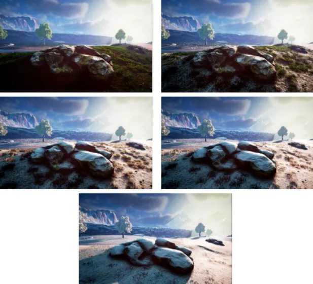
Figure 3.1: Transitions of snow cover without displacement.
Image sequences that show snow transition on rocks, can be seen in Figure 3.1.
3.2.2
Sun Direction Function
In real world, snow covers that are facing towards sun tend to melt faster than snow covers that do not see sunlight. Similarly, in a rainy environment, mosses on rocks tend to grow on the side that sees least amount of sunlight because, sun
makes mosses dry and inhabitable. Equation 3.5 imitates the mentioned event.
fs(p) = Clamp((N • SunDirection) + SunIntensity). (3.5)
Although it seems like a minor detail, overall impact of the sun to the environment cannot be ignored. The influence of the sun to snow and mosses can be observed in the following images Figure 3.2:
(a) The snow accumulation without the
sun direction function (b) Impact of the sun on the accumulation
(c) Same rock in (b) from behind
Figure 3.2: Impact of the sun direction.
3.2.3
Wind Direction Function
Global wind has a huge role to get impression of blizzards. Even though wind is directional, to make it more randomized panning noise texture is used with two different phases.
To use the texture map with specific UV coordinates, one must use the fol-lowing function in shading languages: texture(myTextureSampler, UV) Therefore, this notation will be used to make the wind map generation equation more clear.
Panner(h, v, time) is a function that pans uv coordinates h unit horizontally and v units vertically (time in seconds).
The wind flow equation is as follows:
fpan(h, v) = texture(FlowTexture, Panner(h, v, time)),
fWindDirection(d) = fpan(d.x, d.y) + 0.5 · fpan(d.y, d.x).
(3.6)
Equation 3.6 generates directional wind parallel to the ground. Even though two phased noise map is used to create a randomized flow, the main controller is still the input direction.
The wind influence equation is as follows:
fw(p) = Clamp(N • fWindDirection(Direction · p) + WindIntensity). (3.7)
Equation 3.7 applies wind only to the snow covered parts of the object. The more the object has snow, the more visible the wind become because as the snow gets thicker, upper parts remain softer and have more tendency to be affected by wind. The resulting images can be seen in Figure 3.3.
Figure 3.3: The wind blow phenomena on snow.
3.2.4
Height Function
The height function adds more snow to objects that have more altitude compared to the ones having low altitude. The aim of this function is to make mountains have more snow than the ground level (Equation 3.8).
fheight(p) = Clamp((ObjectPosition.Z − MinHeight)/(MaxHeight − MinHeight)).
(3.8) In Equation 3.8, MinHeight and MaxHeight are determined by the ground level and peak position of the terrain. However, offsetting M inHeight to a higher position can make the ground level not impacted by snow. This may be desirable if the ground level is beach and developers want to simulate snow only on the higher locations. Figure 3.4 shows the impact of the height.
Figure 3.4: The effect of the height function on the terrain.
Equation 3.9 gives the inverted value of the function for moss cover in Equation 3.8:
fheightinv(p) = 1 − fheight(p). (3.9)
According to Equation 3.9, more pressure in air brings more damp and better habitat for moss. Therefore, it is more likely to have moss at lower altitude.
3.2.5
Displacement Function
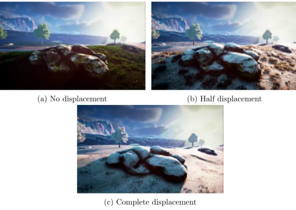
The displacement of snow is determined by the weather prediction function, how-ever more variation is added by using an extra low contrast noise. The displace-ment function is as follows Equation 3.10.
fd(p) = (Clamp(NoiseMap + 0.75) · fp(p) · MaxSnowHeight) • N . (3.10)
High contrast noise may cause holes on the snow surface therefore, brightness of the NoiseMap is increased by 0.75 and clamped to make it overall closer to less contrasted white value. MaxSnowHeight determines snow height in terms of centimeters. It can be adjusted for different objects in the scene so that some objects are covered with less snow. In the test scene, all objects use 25 cm
(a) No displacement (b) Half displacement
(c) Complete displacement
Figure 3.5: Impact of the displacement function.
MaxSnowHeight. Figure 3.5 shows the effects of the displacement compared to the non-displaced version.
In the current implementation displacement is added to vertices in the direction of their normal as a position offset and the weather prediction function determines areas that need offsets. At first thought, this idea may cause sharp unnatural displacements. However, in Equation 3.4, 3rd power of the end result is taken and this makes the displacement relatively smooth.
Another option is using this function in conjunction with tessellation, but tessellating an object close to observer cost more than covering the whole scene with snow. Moreover, most of the times its quality compared to offsetting is slight and does not justify its cost. Still, if final product is only targeting for high end computers, it may be usable.
3.2.6
Terrain Orientation Function
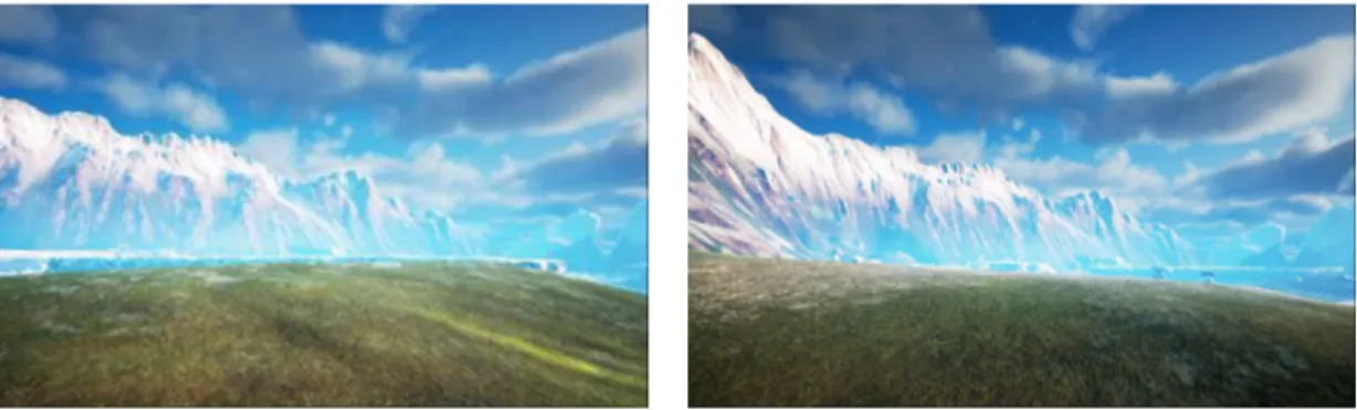
Converting a height map into a slope map requires lot more computation than other functions, therefore it can be used as an optional function to call rather that essential. However, its results affect objects on the terrain in an interesting way. If an object is positioned on an angled surface of the terrain, snow accumulate more on the faces of object that are closer to the terrain than the faces that are far. This makes object blend more with the terrain. The idea of this function comes from snowy mountains, in real life rocks on the high mountains blend with terrain by snow cover. This phenomena can be seen in Figure 3.6:
(a) Rock from downside (b) Rock from upside
Figure 3.6: The position on the terrain affects the direction of the snow coverage.
The first phase is detecting our location on the terrain (Equation 3.11). The scale of the terrain is the only thing needed to detect location of the given object in the shader.
fCoord(p) = WorldPosition/HeightmapScale. (3.11)
In the second part of the Equation 3.12, slopes of the terrain are acquired from height map. The height map consists of only the altitude information, therefore, getting the slope information from the terrain is little tricky. Firstly, the original height map is shifted 0.05 unit horizontally, then its values are subtracted from the original height map. Then a similar operation is performed vertically. Then the cross product of 2 new maps is taken. At the end, similar approach is used to
acquire a normal map from a bump map, but in the current slope map offsetting is more extreme.
fOriginal(p) = texture(Heightmap, fCoord(p)),
fHShift(p) = texture(Heightmap, ((0.05, 0) + fCoord(p))),
fVShift(p) = texture(Heightmap, ((0, 0.05) + fCoord(p))),
fSlope = (1, 0, Intensity · (fHShif t(p) − fOriginal(p)))×
(0, 1, Intensity · (fV Shif t(p) − fOriginal(p))).
(3.12)
In Equation 3.13, the slope information is applied to the object.
fTerrain(p) = ((fSlope· (1, 1, 0)) • N ) · (T N • (0, 0, 1)) · intensity. (3.13)
3.2.7
Weather Transition Function
The weather transition function adds noisy edges to snow, ice and moss while in transition stage. As it can be seen in Figure 3.7, noisy edges look more natural and randomized.
Figure 3.7: The moss is covering a rock, note that edges of the moss seem natural.
Equation 3.14 is used in the scene in Figure 3.7 for moss cover effect.
fTransition(p) = Clamp(NoiseMap − 1 + 3p), (3.14)
where NoiseMap is a noise texture and p is progression value that comes from the weather prediction function.
3.3
Wetness Function
The wetness function is applied only if it is raining and it is independent of other weather conditions. For example, it can be both applied to snowy, mossy and frozen objects if following conditions are met in Equation 3.15.
fWetness= Temperature > 0 & Precipitation > 0. (3.15)
The wetness function affects the individual properties of material such as; diffuse, roughness and normal map in different ways. As it can be seen in real
life, wet objects tend to be more darker, therefore diffuse channel of the material is toned down to %70. In the following set of equations, precipitation amount is always denoted as p which is a float value in between 0 and 1. The diffuse formula is given as (Equation 3.16).
fWetnessD(Diffuse, p) = Diffuse · Lerp(1, 0.7, p). (3.16)
In Equation 3.17, roughness of the materials is toned down as the precipitation amount increases because water is a very smooth material.
fWetnessR(Roughness, p) = Clamp(Roughness − p). (3.17)
In the final step of the wetness (Equation 3.18) a panning normal map is added to the original normal map to achieve flowing water effect.
fWetnessN(Normal, p) = Normal + Pan((p · 0.5, p · 0.01)) · (1, 1, 0). (3.18)
The wetness function under different weather conditions can be seen in Fig-ure 3.8.
(a) Dry
(b) Rainy
3.4
Detail Mask Function
The detail mask function can be used to generate details on objects in early stages of snow cover. It is generated from the diffuse map by creating a mask so that darker areas are filled with snow earlier compared to lighter areas. This comes from the assumption that darker areas in the texture are small cavities. At first, the desaturation operation is applied as described in Equation 3.19, because most of the objects are colored, then resulting values are clamped to get the final result.
~
d = (0.3, 0.59, 0.11),
fDesaturate(in, p) = p · ( ~d · in) + (1 − p) · in,
fDetailMask(Diffuse, p) = Clamp(fDesaturate(Diffuse, p)). (3.19)
(b) Darkest areas in (a) are covered with snow
(d) Complete snow cover using only detail mask
Figure 3.9: The effect of the detail mask function.
The detail mask can be also used for an alternative purpose, as a snow texture. Because, when the diffuse channel is desaturated and its brightness is increased then it seems like a snow texture. Even more interestingly, since every object has a unique diffuse texture, snow seems more randomized between different objects. Even though weather condition renderings are generated, their values are calculated in a way to make sure they are very close to real life measured data. Therefore, the resulting textures are clamped to real snow diffuse reflectance value which is 0.9 [1].
3.5
Frost Mask Function
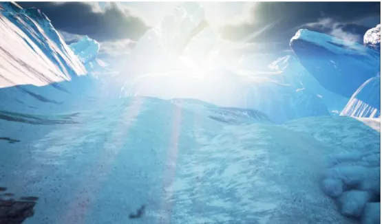
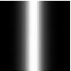
The frost mask is used specifically for rivers to simulate interactive frozen effect from sides to center. Following gradient texture is used to create the interactive frozen effect (see Figure 3.10). The power of this gradient creates necessary animation for the frozen water, in Equation 3.20. Different phases of a frozen river can be seen in Figure 3.11.
Figure 3.10: The effect of the frost mask function.
(a) River before starting to freeze
(c) Side of the river is frozen and its progressing towards to the middle
(d) Whole river is frozen
Chapter 4
Evaluation
4.1
Rendering Quality
The current implementation uses the PBR approach, therefore to evaluate results, real measured data is used from “Art and Rendering of Remember Me” GDC Vault 2013 [1]. Table 4.1 shows the real life scanned values of snow, moss, and ice.
Table 4.1: Measured reflectance values of snow, green grass and ocean ice from “Art and Rendering of Remember Me” GDC Vault 2013 [1].
Material Snow Green Grass Ocean Ice Reflectance Value 0.9-0.95 0.25-0.53 0.5 -0.7
As it can be seen in Table 4.1, resulting color values in shaders are enforced to stay in between targeted values.
4.2
Performance
In the test phase, two different computers are used: one with medium and the other with high performance. Specifications of each computer can be seen in Table 4.2.
Table 4.2: Specifications of A: high performance, and B: medium performance computers.
CPU RAM GPU SSD
A AMD Fx 8350 4.2 GHz 16 GB Nvidia GTX980TI 256 GB SSD B Intel Core i7 4700HQ 3.4 GHz 16 GB Nvidia GTX860M 256 GB SSD
The best way to analyze current implementation is testing the same scene with and without weather shaders. In the following tables, both computers run scenes at 1920 times 1080 resolution.
Table 4.3 depicts the results for the scene Figure 4.1. For Computer A, the overhead of using weather shaders in Scene 1 for Computer A is 0.2 ms, for Computer B, it is 0.4 ms.
(a) Without weather shaders (b) With weather shaders
Figure 4.1: Performance test: Scene 1.
Table 4.3: Average frame time in milliseconds for Scene 1.
Computer Without shaders With shaders
A 9.5 ms 9.7 ms
Table 4.4 depicts the results for the scene Figure 4.2. For Computer A, over-head of using weather shaders in Scene 2 for Computer A is 0.2 ms, for Computer B, it is 0.3 ms.
(a) Without weather shaders (b) With weather shaders
Figure 4.2: Performance test: Scene 2.
Table 4.4: Average frame time in milliseconds for Scene 2.
Computer Without shaders With shaders A 10.1 ms 10.3 ms B 34.4 ms 34.7 ms
Table 4.5 depicts the results for the scene Figure 4.3. For Computer A, over-head of using weather shaders in Scene 1 for Computer A is 0.2 ms, for Computer B, it is 0.5 ms.
(a) Without weather shaders (b) With weather shaders
Table 4.5: Average frame time in milliseconds for Scene 3.
Computer Without shaders With shaders
A 9.3 ms 9.5 ms
B 32.4 ms 32.9 ms
Consequently, in all tests performance cost is far less than the targeted one millisecond for both Computer A and B. For Computer A average execution time is 0.2ms, For computer B average execution time is 0.4 ms.
Chapter 5
Results
5.1
Environments
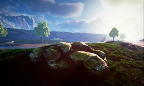
In this section, usage of current method in an actual scene is examined. The summer environment is default and all environmental assets that are prepared for summer, are ready to work. A sample summer scene can be seen in Figure 5.1.
In the following sections, the impact of snow and rain will be examined. How-ever, particle snow and rain effects are removed for better observation.
5.1.1
Snowy Environments
Snow accumulation only occurs in ideal conditions where temperature needs to be less than or equal to zero and there needs to be precipitation. However, it is possible to see snow in temperatures above zero degrees but melting takes place. The frost occurrence is independent from precipitation and less than zero degrees is enough for river to start freezing.
Figure 5.2: Natural snow cover on rocks.
In Figure 5.2, even though the snow texture is generated, it can be seen that snow on rocks seem very natural and randomized. Moreover, snow accumulates less on the surfaces that are directly facing towards sun. Complete equation of the weather prediction function is very suitable to be used with complex shaped meshes such as rocks because all impacts of sub-functions can be observed.
(a) No Snow
(c) Snow starts rising and foliage density starts to decrease
(d) Snow reached its maximum height and foliage density is severely decreased
Figure 5.3: Progression of the snow coverage on terrain.
Currently, foliage uses only detail mask component of the weather prediction function. However, foliage density on the ground decreases as weather becomes more cold and snow starts to rise on the ground. Figure 5.3 depicts the impact of snow on foliage.
Figure 5.4: Snowy mountains.
Figure 5.5: The detail mask function is covering the terrain with snow.
Terrain uses different prediction functions for its different materials. For its cliff and rocky parts, it uses same complete version of the weather prediction function. However, for grassy parts, it uses only detail, height and wind functions, which
is little reduced version of the complete equation. Results of the height function can be observed in Figure 5.4. The detail mask on the terrain can be seen in Figure 5.5. Wind blow effect on terrain can be observed in Figure 5.6. Even though blowing wind phenomena can be seen clearly in an animation, it is hard to see in a still picture. In Figure 5.6, varied color changes on the terrain are blowing wind phenomena.
Figure 5.7: The frozen road.
Although most objects in the scene are affected by the snow displacement, some objects do not. The first one is foliage, due to the fact that in the real-time scenes, foliage use alpha planes rather than detailed leaf meshes, they have very low polygon count and displacement causes artifacts. Furthermore, river and road are also not effected by snow, to observe frost effect clearly. The frozen road can be observed in Figure 5.7 and the frozen river can be observed in Figure 5.8.
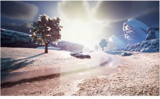
Figure 5.8: A snowy scene with particle effects.
In Figure 5.8, the final result with snow particles is illustrated. In snowy environments, particle effects only run near the observer, with max distance of eight meters.
5.1.2
Rainy Environments
Rain affects environment, if temperature is more than zero degree and there is precipitation in the scene, the wetness function is applied to any scene object regardless of their material. For example, if whole environment is covered with snow and temperature rises, then rain starts, the wetness function also affects the snow on the ground and slowly melts it. In Figure 5.9, rain phenomena can be observed. Most noticeable features of wetness are as follows; it makes diffuse color darker, reduces roughness value and emerges flowing micro normal effect.
(a) Dry
(b) Rainy
Figure 5.9: The same scene with both dry and rainy weather conditions.
If it is raining, after some time, mosses start covering the rocks. Slightly modified version of the weather prediction function is used for moss. Moss grows on the sides of the objects that are exposed to least amount of sun light because it makes moss dry. Similarly, moss tend to grow on lower altitudes, because
having more pressure in the air makes more damp and better living conditions. In Figure 5.10, moss coverage can be observed.
Figure 5.10: When rain stops, mosses start to fade from rocks and accumulated water starts to evaporate from the ground.
In Figure 5.11, the moss texture is generated similar to snow by using detail mask, at the end of detail mask function, its value is multiplied by a green value. PBR values of moss could not be found, therefore adjustments were made for targeted diffuse color and roughness as if they were grass. Therefore, end clamp operation is done to make sure color and roughness values stay in the valid interval.
Figure 5.11: Transitions of the moss cover on rocks.
In Figure 5.12, water accumulation on roads can be seen. The places of accu-mulation are determined by a high contrast noise. The rain accumulates if and only if world space normal of the road is facing upwards and within eight degrees of tolerance.
(a) Dry
(b) Rainy
Figure 5.12: Water accumulates on the ground, when it is raining.
In Figure 5.13, the final result with rain particles is illustrated. In rainy en-vironments, particle effects only run near the observer, with a max distance of eight meters.
Chapter 6
Conclusion
The main goal of this thesis is to achieve good looking weather conditions that have minimal overhead rather than complex physically correct simulations. Con-sidering performance, extra cost to render weather functions are less than 1 ms on both tested systems. Loosely coupled integration allows this technique to be used in any real-time engine that supports PBR without breaking down the original rendering system and previously created environments.
Considering simulation results, the weather prediction function generates nat-ural looking accumulation as if they were physically simulated for both snowy and rainy environments. Using diverse factors in prediction brings desired ran-domness to an environment. Even though generated textures are used for snow and moss, their values are adjusted to be as close to the real life values.
There are several drawbacks to use the current prediction model. In the current system, all objects in the scene need to be scanned to determine objects that are in closed areas. This operation is done by raycasting to the skybox. If the raycast is unable to hit the sky, the original shader is loaded to the object. This operation is executed while loading a scene, therefore it has no impact to the performance. Additionally, more detailed prediction models can be used, because current performance overhead is very low and there is still much room for more
complex prediction models.
There are several potential future extensions that can improve the current ap-proach. Firstly, Distance Field Ambient Occlusion (DFAO) data can be used in the weather prediction function. DFAO is a new real-time ambient occlusion ren-dering technique that is capable of creating large occlusion shadows. Therefore, it can be used to detect areas that are less likely to be affected by snow. For instance, large trees can create areas near their roots which are less affected by snow and rain.
Secondly, implementing more realistic particle emitters for snow and rain can improve the overall mood of the scene. Real wind patterns can be analyzed and better emitters can be implemented.
Bibliography
[1] S. Lagarde and L. Harduin, “The art and rendering of Remember Me,” GDC Europe Vault Course Notes, 2013.
[2] B.-T. Phong., “Illumination for computer generated pictures,” Communica-tions of the ACM, vol. 18, no. 6, pp. 311–317, June 1975.
[3] W. Matusik, H. Pster, M. Brand, and L. McMillan, “A data-driven re-flectance model,” ACM Transactions on Graphics, vol. 22, no. 3, pp. 759–769, July 2003.
[4] B. Burley, “Physically-based shading at Disney,” SIGGRAPH 2012 Course Notes, 2012.
[5] B. Karis, “Real shading in Unreal Engine 4,” SIGGRAPH 2013 Course Notes, 2013.
[6] R. L. Cook and K. E. Torrance, “A reflectance model for computer graphics,” Computer Graphics (SIGGRAPH 81 Conference Proceedings), vol. 15, no. 3, pp. 307–316, July 1981.
[7] C. Schlick, “An inexpensive BRDF model for physically-based rendering,” Computer Graphics Forum, vol. 13, no. 3, pp. 149–162, 1994.
[8] S. Lagarde, “Spherical Gaussian approximation for Blinn-Phong, Phong and Fresnel,” Computer Graphics Forum, June 2012.
[9] P. Fearing, “Computer modelling of fallen snow,” In Proceedings of the ACM SIGGRAPH, pp. 37–46, 2000.
[10] H. Haglund, M. Andersson, and A. Hast, “Snow accumulation in real-time,” In Proceedings of the SIGRAD, pp. 11–15, 2002.
[11] P. Ohlsson and S. Seipel, “Real-time rendering of accumulated snow,” In Proceedings of the SIGRAD, pp. 25–32, 2004.
[12] T. Morriya and T. Takahashi, “Real-time computer model for wind-driven fallen snow,” In Proceedings of the ACM SIGGRAPH ASIA, pp. 15–18, 2010.