KAD˙IR HAS UNIVERSITY
GRADUATE SCHOOL OF SOCIAL SCIENCES
THE EFFECT OF MONETARY POLICY ON FOREIGN TRADE BALANCE IN TURKEY, IN PARTICULAR THROUGH CREDIT CHANNEL
GRADUATE DISSERTATION
G ¨URB ¨UZ KIRAN
THE EFFECT OF MONETARY POLICY ON FOREIGN TRADE BALANCE IN TURKEY, IN PARTICULAR THROUGH CREDIT CHANNEL
G ¨URB ¨UZ KIRAN
Submitted to the Graduate School of Social Sciences in partial fulfillment of the requirements for the degree of
Doctor of Philosophy in
ECONOMICS
KADIR HAS UNIVERSITY April, 2017
ABSTRACT
THE EFFECT OF MONETARY POLICY ON FOREIGN TRADE BALANCE IN TURKEY, IN PARTICULAR THROUGH CREDIT CHANNEL
G¨urb¨uz Kıran
Doctor of Philosophy in Economics Advisor: Asst. Prof. Dr. Sabri Arhan Ertan
April, 2017
The paper is about the possible effect of monetary policy on the post 2001 lending boom, and the related current account deficit in Turkey. In the analysis, VAR, ARDL, IRF and Granger causality tests have been used. Moreover, the effect of the policy, in particular through real interest rates, has also been analyzed separately on consumer, public and other (business) loans. Even after taking the influence of global risk appetite as the factor for funds flow into emerging markets, including Turkey, into the consideration, it has been shown that monetary policy seems to affect current account and its main component of foreign trade balance via its influence on loan growth, especially through consumer and other (business) loan channels.
Keywords: Monetary Policy, Credit (Loan) Channel, Foreign Trade Bal-ance
¨ OZET
THE EFFECT OF MONETARY POLICY ON FOREIGN TRADE BALANCE IN TURKEY, IN PARTICULAR THROUGH CREDIT CHANNEL
G¨urb¨uz Kıran Ekonomi Doktora
Danı¸sman: Yard. Do¸c. Dr. Sabri Arhan Ertan Nisan, 2017
Bu ¸calı¸sma T¨urkiye’deki para politikasının 2001 yılı sonrasında g¨ ozlem-lenen kredi geni¸slemesi ve cari a¸cık ¨uzerindeki muhtemel etkileri ¨ uzeri-nedir. Ara¸stırmada, VAR, ARDL, IRF ve Granger nedensellik test-leri kullanılmı¸stır. Bu kapsamda, reel faiz oranı ile temsil edilen para politikasının t¨uketici, kamu ve di˘ger ticari kredileri ¨uzerine etkileri ince-lenmi¸stir. Sonu¸c olarak, T¨urkiye gibi y¨ukselen / geli¸sen ekonomilere fon akı¸sının temel fakt¨orlerinden olan k¨uresel risk i¸stahı ve benzeri de˘gi¸skenler de dikkate alındı˘gında, para politikasının nihai olarak cari denge ve onun ana bile¸seni dı¸s ticaret dengesini di˘ger ticari ve t¨uketici kradiler kanalı yoluyla etkiledi˘gi g¨ozlemlenmi¸stir.
Acknowledgements
Firstly, I would like to express my sincere gratitude to my advisor Asst. Prof. Dr. Sabri Arhan Ertan for the continuous support of my Ph.D study and related research, for his patience, motivation, enthusiasm, and immense knowledge. His guidance helped me during the entire period of research and writing of this thesis. I deeply appreciate it all.
Besides my advisor, I would like to thank the rest of my thesis committee: Assoc. Prof. Dr. Mustafa Eray Y¨ucel, Prof. Dr. Burak Salto˘glu, Assoc. Prof. Dr. K. Ali Akkemik and Asst. Prof. Dr. Hasan Tekg¨u¸c; and additionally to Assoc. Prof. Dr. ¨Ozg¨ur Orhangazi, for their insightful comments and encouragement, but also for the hard questions which have led me to widen my research from various perspectives.
Moreover, I would like to thank my friends who have provided invalu-able assistance. Finally, I would also like to thank my family: my wife and my parents in particular, for their continuous support and sacrifices throughout the writing of this thesis; without them, it would have not come about.
Contents
1 Introduction 1
2 Models 3
2.1 VAR (Vector Auto Regressive) Model . . . 3
2.1.1 Granger Causality . . . 4
2.1.2 Impulse Responses . . . 5
2.1.3 Variance Decompositions . . . 5
2.2 Error Correction Model (ECM) . . . 5
2.3 Auto Regressive Distributed Lag (ARDL) Model . . . 7
2.4 Seasonality . . . 8
2.4.1 Seasonality Tests . . . 8
2.4.2 TRAMO SEAT Methodology . . . 11
2.5 Structural Break Tests . . . 11
3 Literature Review 14 3.1 Current Account Deficits: How bad are they? . . . 14
3.2 The Role Of Credit Expansion On Financial Stability . . . 17
3.3 Monetary Policy Transmission Channels Covering Banks . . . 20
3.4 Determinants of Consumption in a Macroeconomic Environment . . . 21
3.5 Determinants of Investment Expenditures in Macroeconomic Environ-ments . . . 24
3.6 Effects of Monetary Policy on Foreign Trade and External Balances for Advanced Economies . . . 26
3.7 Effects of Monetary Policy on Foreign Trade and External Balances for Emerging Economies . . . 30
3.8 Studies about Turkey . . . 34
4 THEORETICAL BACKGROUND 37 4.1 SHORT TERM EQUATIONS . . . 37
4.1.1 Loan Market Equilibrium . . . 37
4.1.2 Money Market (LM) Equilibrium . . . 37
4.1.3 Foreign Exchange Market Equilibrium . . . 38
4.1.4 Good Market (IS) Equilibrium . . . 38
4.2 LONG TERM (STEADY STATE) EQUATIONS . . . 38
4.2.1 Loan Market Equilibrium . . . 38
4.2.2 Money Market (LM) Equilibrium . . . 39
4.2.3 Foreign Exchange Market Equilibrium . . . 39
4.2.4 Good Market (IS) Equilibrium . . . 39
6 RESULTS 53 6.1 Effect of Credit (Loan) Transmission Channel of Monetary Policy on
FTB . . . 53
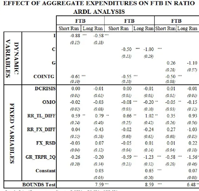
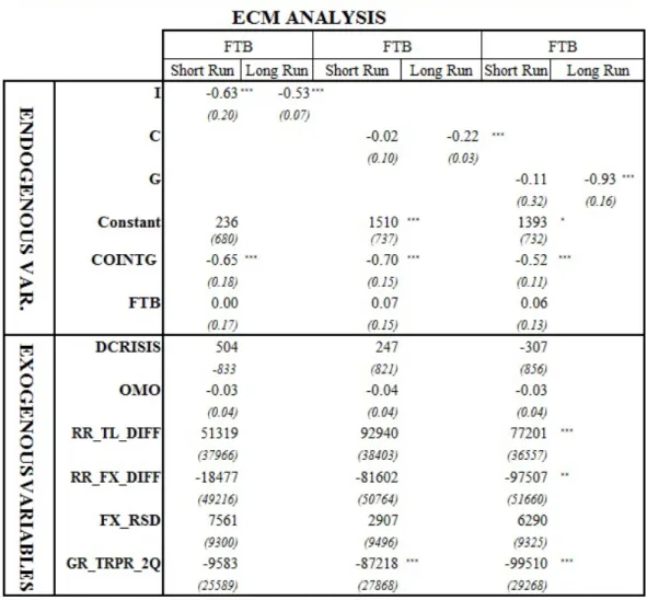
6.2 Effect of Aggregate Expenditures on Foreign Trade Balance . . . 58
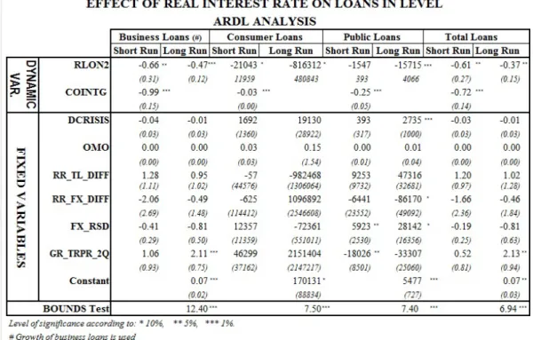
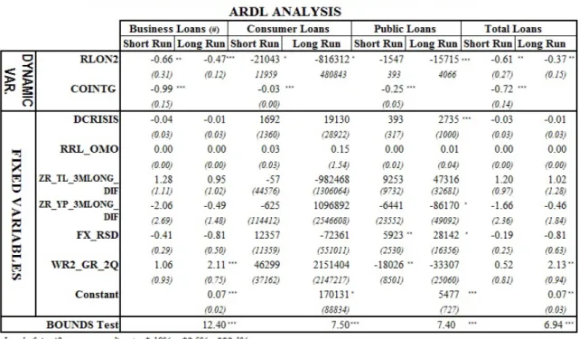
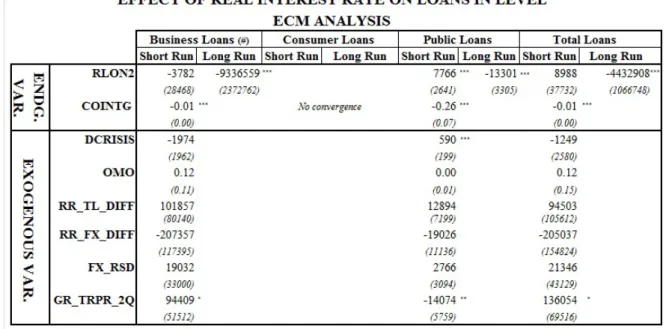
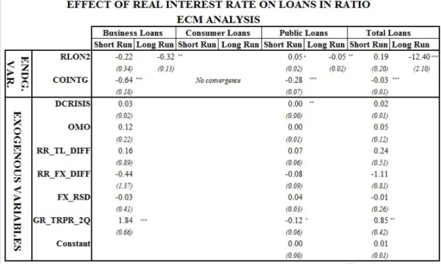
6.3 Effect of Real Interest Rate on Loans . . . 63
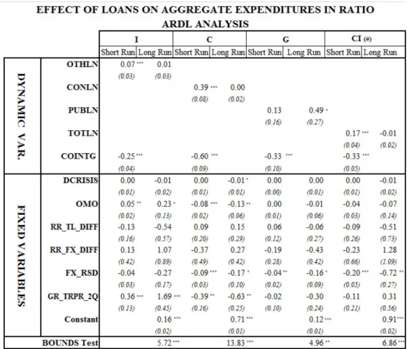
6.4 Effect of Loans on Aggregate Expenditures . . . 67
6.5 Robustness Checks . . . 73
7 CONCLUSION 81 8 REFERENCES 83 9 APPENDIX 89 9.1 Impulse Response Tables of VAR on Credit Channel, Ratio Analysis . 89 9.2 Impulse Response Tables of VAR on Credit Channel, Level Analysis . 95 9.3 Impulse Response Tables of VAR on Credit Channel with all station-ary variables, Ratio Analysis . . . 101
9.4 Impulse Response Tables of VAR on Credit Channel with all station-ary variables, Level Analysis . . . 106 9.5 Impulse Response Tables of VAR Effects of Real Interest Rate on Loans111
List of Tables
6.1 Effects of Loans Channel To FTB in Level, ARDL Analysis . . . 57 6.2 Effects of Loans Channel To FTB in Ratio, ARDL Analysis . . . 58 6.3 Effect of Aggregate Expenditures On FTB in Level, ARDL Analysis . 60 6.4 Effect of Aggregate Expenditures On FTB in Ratio, ARDL Analysis . 61 6.5 Effect of Aggregate Expenditures On FTB in Level, ECM Analysis . 62 6.6 Effect of Aggregate Expenditures On FTB in Ratio, ECM Analysis . 63 6.7 Effect of Real Interest Rate On Loans in Level, ARDL Analysis . . . 65 6.8 Effect of Real Interest Rate On Loans in Ratio, ARDL Analysis . . . 65 6.9 Effect of Real Interest Rate On Loans in Level, ECM Analysis . . . . 66 6.10 Effect of Real Interest Rate On Loans in Ratio, ECM Analysis . . . . 67 6.11 Effect of Loans On Aggregate Expenditures in Level, ARDL Analysis 69 6.12 Effect of Loans On Aggregate Expenditures in Ratio, ARDL Analysis 70 6.13 Effect of Loans On Aggregate Expenditures in Level, ECM Analysis . 71 6.14 Effect of Loans On Aggregate Expenditures in Ratio, ECM Analysis . 72 6.15 Summary of the Analyses in Level . . . 79 6.16 Summary of the Analyses in Ratio . . . 80
List of Figures
9.1 Impulse Response Graphics of Total Loans for All Variables, Ratio Analysis . . . 90 9.2 Impulse Response Graphics of Total Loans, Ratio Analysis . . . 91 9.3 Impulse Response Graphics of Other (Business) Loans, Ratio Analysis 92 9.4 Impulse Response Graphics of Consumer Loans, Ratio Analysis . . . 93 9.5 Impulse Response Graphics of Public Loans, Ratio Analysis . . . 94 9.6 Impulse Response Graphics of Total Loans for All Variables, Level
Analysis . . . 96 9.7 Impulse Response Graphics of Total Loans, Level Analysis . . . 97 9.8 Impulse Response Graphics of Other (Business) Loans, Level Analysis 98 9.9 Impulse Response Graphics of Consumer Loans, Level Analysis . . . . 99 9.10 Impulse Response Graphics of Public Loans, Level Analysis . . . 100 9.11 Impulse Response Graphics of Total Loans, Ratio Analysis . . . 102 9.12 Impulse Response Graphics of Other (Business) Loans, Ratio Analysis 103 9.13 Impulse Response Graphics of Consumer Loans, Ratio Analysis . . . 104 9.14 Impulse Response Graphics of Public Loans, Ratio Analysis . . . 105 9.15 Impulse Response Graphics of Total Loans, Level Analysis . . . 107 9.16 Impulse Response Graphics of Other (Business) Loans, Level Analysis 108 9.17 Impulse Response Graphics of Consumer Loans, Level Analysis . . . . 109 9.18 Impulse Response Graphics of Public Loans, Level Analysis . . . 110 9.19 Impulse Response Graphics of Total Loans to Real Interest Rate . . . 112 9.20 Impulse Response Graphics of Other (Business) Loans to Real Interest
Rate . . . 113 9.21 Impulse Response Graphics of Consumer Loans to Real Interest Rate 114 9.22 Impulse Response Graphics of Public Loans to Real Interest Rate . . 115
List of Abbreviations
AR: Auto Regressive
ARDL: Auto Regressive Distributed Lag
C: Consumption Expenditures
CA: Current Account
CBTR: the Central Bank of the Republic of Turkey
CDS: Credit Default Swap
CPI: Consumer Price Index
ECM: Error Correction Model
EMBI+: Emerging Markets BondIndex+
EU: European Union
EUR: Euro
FAVAR: Factor Augmented Vector Auto Regression FDI: Foreign Direct Investment
FED: Federal Reserve
FOMC: Federal Open Market Committee FTB: Foreign Trade Balance
FX: Foreign Exchange
G: Government Expenditures
GARCH: Generalized Autoregressive Conditional Heteroskedasticity
GDP: Gross Domestic Product
GMM: Generalized Method of Moments HFI: High Frequency Identification
I: Investment Expenditures
IS - LM: Investment Savings - Liquidity Money
M: Imports
OLS: Ordinary Least Square)
OMO: Open Market Operations
RER / REER: Real Exchange Rate
RHS: Right Hand Side
ROM: Reserve Option Mechanism
RPI: Retail Price Index
SSR: Sum of Squared Residuals
TOT: Terms of Trade
TRY / TL: Turkish Lira
TSI: Turkstat, Turkish Statistical Institute
UK: United Kingdom
USA: United States of America USD: United States Dollar VAR: Vector Autoregressive
VECM: Vector Error Correction Model
VIX: Chicago Board of Exchange Volatility Index
WW: World War
1
Introduction
There have been several papers published related to the risk of excessive loan growth on financial stabilities (i.e. their role in financial crises), especially after the 2007 mortgage crisis. In this respect, the lending boom, in particular the consumer lending boom (including credit card receivables) in Turkey of the last decade, whose size has more than quadrupled, has received particular attention.
Likewise, with the policy change in Q4 2010 in Turkey (following the successful inflation targeting regime applied since the February 2001 crisis, when short-term interest rates have been used as the main policy tool,1 while foreign exchange[FX] rates are also allowed to float) CBTR has started a new monetary policy. Thus, the bank, apart from setting the policy rate to get price stability, has started to use other tools like Reserve Requirement Ratios, where further flexibility is ensured by Reserve Option Mechanism (ROM), Open Market Operations, and TRY interest rate corridor2, to maintain financial stability, through loans and FX rate channel[55,
pp. 2-5]. Primarily, the bank has tried to control the current account deficit, mostly through foreign trade deficit as its main component, by means of limiting excessive loan growth and excessive TRY exchange rate appreciation[42, pp. 14-15].
However, in terms of the foreign trade deficit, there are also some important points to make. Initially, there are some expenditures which are mainly out of control of the CBTR, but which Turkish production sectors depend on such as energy. Similarly, due to the structural nature of its open economy, exports and the growth of Turkey are significantly dependent on the imports of intermediate and capital goods.
Therefore, in this study, the effect of monetary policy on foreign trade balance through the credit channel has been analyzed, in order to shed some more light onto this process, so that questions like: whether rather than controlling overall credit growth, would it make more sense to control consumer loans? might be answered with more evidence.
Hence, the second section of the thesis comprises the main time series economet-ric models which have been used. In this respect, definitions and main properties, together with the strengths and weaknesses of these models have been presented. This section starts with the ”Vector Auto Regressive (VAR) Model”, which is fol-lowed by ”Error Correction (EC)” and ”Auto Regressive Distributed Lag (ARDL)” models respectively. Afterwards, the section comprises ”Seasonality” as one of the
1interest rates are adjusted in response to deviations of inflation from a targeted path
2Interest rate corridor is defined as the margin between the overnight lending and borrowing
critical concepts in time series analysis, and it ends with the Structural Break Test which has been applied in the study as well.
The literature review has been situated in section 3 of the thesis. It starts with the current account deficit issue. Three main approaches evolved in the post second World War era about the negativity and the sustainability of deficits have been presented. The section continues with a review of the literature about the role of credit expansions on financial stability (their roles in the past crises), for both advanced and emerging economies like Turkey. Next, there follows a part related to monetary policy transmission channels, covering banks. Afterwards, the literature about the determi- nants of consumption and investment expenditures respectively have been presented . The following section consists of the literature about the effects of monetary policy on foreign trade and external balances for advanced and emerging economies. Finally, the related studies about Turkey have also been presented.
Section 4 contains the theoretical background. A small open economy IS - LM model (a version of the Mundell-Fleming model)with floating exchange rates has been used as a base template, to which loans have been added to represent the Turkish economy. Furthermore, the response of the model variables to a monetary shock and both short and long run equilibrium conditions have been analyzed.
Variables used in the analyses of the thesis have been presented in section 5. The section contains various details such as the sources, the types (whether they have been used as exogenous or endogenous variables), seasonality and stationarity of these variables.
The sixth section is also about the results of the analyses carried out on both real values of the variables3, and the ratio of real values over real GDP4. Initially,
the results related to the effect of the loan transmission channel of monetary policy have been presented, where in addition to the total loans, the loan channel has also been examined through the composition of consumer, public and other (business) loans. The methods used at this stage are VAR and ARDL. Then the results of the studies of three subparts of the transmission channel have been reported in three subsections: the effect of aggregate expenditures on Foreign Trade Balance, the effect of real interest rate on loans and the effect of loans on aggregate expenditures. The methods used at these stages are also VAR, ARDL and ECM. The section ends with the robustness check subsection, where through the inclusion of several related variables(such as net FDI, net portfolio investments, oil prices, public budget deficit and variance in global and country risk level), the results of the models have been tested.
In the seventh section, in the light of the results derived, some policy recommen-dations have been suggested, and areas for future research have also been pointed out, and some recommendations for practitioners of time series analysis have been made.
Finally, the impulse-response graphics are also presented in the appendix, cap-tioned as the ninth chapter.
3This is called the level analysis 4This is called the ratio analysis
2
Models
2.1
VAR (Vector Auto Regressive) Model
The first methodology comprises setting up a base VAR model representing the basic monetary relation in an economy, in particular the monetary transmission mechanism by bank loan channel, among the variables like ex-ante overnight real interest rate, variances in several loan stocks (business, consumer, public loans and total loans), macroeconomic expenditures, real effective exchange rate and foreign trade balance and current account balance, with the control of several variables like open market operations, reserve requirements, global mortgage crisis period and local volatility represented through relative standard deviation of nominal exchange rate. It is represented by the following:
Yt = C + p
X
i=1
ΦiYt−i+ BXt+ εt
Where, the components of the vector Yt are the endogenous variables, and Xt are the exogenous variables as their values are determined outside of the model (in other words, they are the control variables). Moreover, the components C and εt are
also the components of constant and error variables respectively.
VAR models were made famous in econometrics by Sims(1980). VAR is indeed a systems regression model, where there is more than one dependent variable, which might be thought of as a hybrid between a simultaneous equations model and an univariate time series model. Compared with these models, VAR models have various advantages:
• They are more flexible than univariate AR (Auto regressive) models since the value of a variable might depend not only on its own lags or combinations of white noise terms but also those of other endogenous variables.
• Using OLS (Ordinary Least Square) separately on each equation is possible, if there are no contemporaneous terms on the RHS (Right Hand Side) of the equations due to the fact that all variables on RHS are predetermined.
• It is not necessary to define which variables are exogenous or endogenous as all variables are endogenous. This allows one the discretion as to how to classify the variables, so there is no need to use and impose identifying restrictions (and use of Hausman-type tests).
• It is often seen that the forecasts of VARs perform better than those of tradi-tional structural models. Probably owing to the ad hoc nature of the restric-tions put on structural models to make sure of aforementioned identification, in several articles [70] it has been claimed that large scale structural models did not perform as well in terms of out-of-sample forecast accuracy.
Besides these advantages, VAR models, however, have several disadvantages and limitations as well.
• All variables of the VAR model need to be stationary. It is not possible to use data in levels and first differences together in the analysis. Hence any infor-mation will be lost in getting any long run relationship among the variables, if differencing is used in order to make non-stationary variables into stationary ones.
• The number of parameters needed to be estimated is quite large. To illustrate, if there are n equations for n variables, together with l lags, then total [n(1+kn)] parameters are required to be estimated. For analyses with rather small sample sizes, this means large standard errors, so wide confidence intervals for the coefficients of the models due to the degrees of freedom issue.
• Generally VARs are a-theoretical models, as they might depend on less use of theoretical background among the variables to monitor the specification of the model. In this respect, sometimes it is not obvious how to interpret their coefficient estimates as well.
2.1.1 Granger Causality
Within VAR models, Granger Causality among the variables has also been tested. A rather simple definition of Granger Causality, in the case of two time-series variables, M and N can be stated as: Variable M is stated to Granger-cause variable N provided that N would be better predicted using the histories of both M and N than it would by using the history of N alone. An absence of Granger Causality can be tested by estimating the following VAR model:
Nt = a0+ a1Nt−1+ ... + apNt−p+ b1Mt−1+ ... + bpMt−p+ ut(1)
Mt = c0+ c1Mt−1+ ... + cpMt−p+ d1Nt−1+ ... + dpNt−p+ et(2)
Then, testing H0 : b1 = b2 = ... = bp = 0, against HA : N otH0, is a test that M
does not Granger-cause N. Likewise, testing H0 : d1 = d2 = ... = dp = 0, against
HA: N otH0, is a test that N does not Granger-cause M. In each case, a rejection of
2.1.2 Impulse Responses
Any responsiveness of the dependent variables in a VAR model to shocks to each one of the (dependent) variables is traced out by impulse response analyses. In this respect, a unit shock (innovation) is applied to the error and the effects on the VAR system over time are analyzed. Furthermore, if the model and the underlying system are stable, any shock should gradually die away. Thus, in this way, any positive and negative effect on the other variables of a change of a variable within the system, and how long it takes for that effect to go through the system is revealed through impulse response analyses.
2.1.3 Variance Decompositions
Variance decompositions provide the proportion of the movements in the dependent variables resulting from their own shocks versus those of other variables in a VAR system. Hence, how much of t step ahead forecast error variance of a given variable is explained by innovations to each independent variable as t = 1, 2, 3.. is determined by variance decompositions. The basis for these analyses is the dynamic structure of VAR models, so due to this dynamic set up, an innovation (shock) given to a variable affects not only itself but is transmitted to other variables in the system. Finally, in both Impulse Response and Variance Decomposition analyses, the or-dering of the variables is important and economic theory is applied at this stage. Moreover, orthogonalization is also used in order to overcome the correlated error terms possibility among the equations in VAR models, as impulse responses and vari-ance decompositions refer to unit shock (innovation) as the errors of one equation only.
2.2
Error Correction Model (ECM)
Error Correction Models are used in order to model long-term relations in time series analyses. In time series analyses, moreover, the notion of stationarity and non-stationarity is essential, as the variables which are stationary are treated dissimilarly to the ones which are non-stationary. Furthermore, variables which have constant mean and constant variance, as well as constant auto covariance for a given lag can be defined as stationary series, more formally[20, p. 367] : a variable y is stationary if it satisfies the following three conditions for t = 1, 2, 3, ..∞
• E(yt) = µ
• E(yt− µ)(yt− µ) = σ < ∞
• E(yt1− µ)(yt2− µ) = µt1−t25, ∀t1, t2
5This is also called weak stationarity or covariance stationary process. There is also strictly
stationary process. This is defined as: the process (yt: t = 1, 2, 3, ..) where for every collection of
time indices 1 < t1< .. < tn the joint distribution of (yt1, ..ytn) is the same as the joint distibution
of (yt1+g, ..ytn+g) for all integers g ≥ 1, thus, the probability of y fallng a specific interval is the
The main results of using nonstationary data (so the differences from stationary data) would be stated as follows:
• Spurious regressions might come out as a consequence of using nonstationary data. For instance when two independent but trending over time variables are regressed on each other, then a regression which seems good under stan-dard measures such as significant coefficient estimates and a high R2 might be obtained, which however is indeed nonsense.
• In regressions among the nonstationary variables, the standard assumptions for the asymptotic analysis would not work so are not valid. That is to state that the F statistic would not follow an F distribution, and similarly t ratios would not follow a t distribution either, and so on.
• Finally, any shocks (or innovations) to a system will die away gradually for stationary series. In other words, the effect of an innovation applied at time t will have a smaller effect at time t+1, then a much smaller effect at time t+2 and onwards. However, this is not the case for nonstationary series, where the innovations will persist infinitively. Hence, compared with the stationary series, the effect of an innovation will not have smaller effects as time goes by. Differencing comes into the picture at this stage. It is one way of converting non-stationary time series into non-stationary ones. The first difference of a variable x is calculated by the difference between the value of x at time t and its value at one period before, and shown as:
4xt = xt− xt−1[20, p.156]
Moreover, assuming this variable becomes stationary, then, it is also stated as inte-grated of order 1. In addition, for any variable that is required by differenced g times in order to be stationary, it is stated to be integrated of order g and is represented by xt ∼ I(g). In this frame a stationary variable can be show as I(0)[20, p. 375] .
Normally, the residuals of I(1) series are also I(1). However, it is also possible that the residuals of linear combinations of some I(1) series are stationary I(0), provided that the variables are cointegrated. Furthermore, theoretically it is reasonable for some variables to have long term relationship with each other, like spot and future prices of assets. A more general definition of cointegration can be presented as the following: Given vt being an m × 1 vector of variables, the elements of vt are stated
to be integrated of order (f,h) provided that: 1. All elements of vt are I(f)
2. There is at least one vector of coefficients β where β0vt is I(f − h)[20, p. 388]
Moreover, the main test which is used to estimate cointegration systems is the Jo-hansen technique. For a system of h variables all of which are I(1), it can be repre-sented as :
where, I stands for identity matrix, and k is the number of lags, then: Π = (Pk
i=1βi) − Ih and Γi= (
Pi
j=1βj) − Ih
The Johansen Method focuses around analysis of Π matrix which can also be inferred as a long run coefficient matrix. The cointegration test among m series is calculated by comparing the rank of Π matrix b its eigenvalues. Finally, this method also allows coefficient restrictions as well to test the cases imposed by theoretical intuitions etc [20, pp. 403-409]. Furthermore, if the series are I(1)6 and there is
coin-tegration among them, then ECM, (if there is more than one coincoin-tegration equation among them, then the model is also called Vector Error Correction Models VECM-) is the appropriate model to analyze, their potential in both long term and short term relationships. A basic two variable model is presented below:
∆mt = β1∆nt+ β2(mt−1− γnt−1) + εt
Here, γ stands for the long run relationship between m and n, as any model based solely on differenced terms (∆) does not lead to any long run equilibrium result. Plus, the short run relationship between changes in n and changes in m is also defined by β1. Finally, the fraction of the previous periods equilibrium error which is corrected
for is also described by β2 (This is also called the speed of adjustment of the ECM
model)[20, pp. 390-391] . Besides this, a VECM with k lags with the cointegration rank r(≤ h) is presented as ∆mt = δ + Πmt−1+ k−1 X i=1 Θi∆mt−1+ εt
where, Π = αβ and α and β are h×r matrices; while, Θ is an h×h matrix[36]
2.3
Auto Regressive Distributed Lag (ARDL) Model
Auto Regressive Distributed Lag (ARDL) Models comprises the cases where the value of a dependent variable depends on the contemporaneous and the previous values of explanatory variables and the previous values of the dependent variable. Hence, an ARDL(p,r) model is represented by the following:
yt = η + p X i=1 γiyt−1+ r X j=0 βjxt−1j + εt where, ε is i.i.d ∀t
These models have become popular in recent years as a method of examining long-run and cointegrating relationships among variables (Pesaran and Shin, 1999)[59] and Pesaran et al. (2001)[60] . In this regard, they allow us to incorporate I(0) and I(1) variables in the same estimation. Apart from these, other basic advantages of the ARDL model are that compared with VAR, ARDL uses a single equation, so requires much fewer parameters to be estimated. Finally, with ARDL, restrictions on the number of lags might separately be applied to each variable unlike the Johansen Method.
6Assuming they turn into I(0) with differencing, so that OLS and its standard procedures for
2.4
Seasonality
Seasonality can be defined as the observed movements in time series, which recur in a year, at particular time points and with similar intensity in a given season. More-over, seasonality can be observed in time series whose frequency is higher than once in a year (like monthly, quarterly etc.). Hence, it is the orderly, though not neces-sarily regular, intra - year movement which results from the changes of the calendar, timing of decisions and the weather, directly or indirectly, via the consumption and the production decisions made by the agent of the economy.[38].
Thus, seasonal movements are likely to be foreseeable. Under normal circum-stances though factors which induce seasonality can gradually change through time as they might not be non-steady, they can be expected to repeat. The main tests used to check is a variable has seasonality or not are presented below:
2.4.1 Seasonality Tests
The Friedman Test (Stable Seasonality Test)
This is a non-parametric method to test whether samples are drawn from the same population or from populations with equal medians. Moreover, in the regression equation the significance of the quarter (in this analysis) effect is tested. the test requires no distributional assumptions and the rankings of the observations are used. The Friedman Test is also described as a stable seasonality test. The test uses initial estimation of the unmodified Seasonal-Irregular component (outliers or seasonal-irregular factors with extreme values) from which l samples are derived (it is 4 as quarterly variables are used in this analysis) of size n1, ..., nl respectively. Each l
represents a different level of seasonality. Here, the fact that seasonality affects only the means of distribution and not their variance is assumed. Moreover, the null hypothesis below is tested under the assumption that each sample is derived from a random variable Xi following normal distribution with mean mi and standard
deviation σ.
H0: m1 = m2= ... = ml
against:H1: mr6= ms for at least one pair (r, s)
Moreover the test applies the following decomposition of the variance:
l X j=1 nj X i=1 (xi,j− ¯x) 2 = l X j=1 nj(¯x.j − ¯x..)2+ l X j=1 nj X i=1 (xi,j− ¯x.j) 2
here, ¯x.j stands for the average of j -th sample. Hence, the total variance is
decom-posed into a variance of the averages due to seasonality and a residual seasonality. Then, the test statistics are calculated as:
F = Pl j=1nj(¯x.j−¯x..)2 l−1 Pl Pnj (x −¯x )2 ∼ F (l − 1, n − l)
Where l 1 and n k represents the degrees of freedom. Finally, If the null hypothesis of no stable seasonality is not rejected at the 0.001 significance level (P ≥ 0.001), then the series is assumed to be non-seasonal.
The Kruskal-Wallis test
This is a non-parametric test used to compare samples from two or more sets. The null hypothesis claims that all quarters (in this analysis) have the same mean. More-over, the Kruskal-Wallis test is run (or excercised)for the final estimate of the un-modified Seasonal-Irregular component in which m samples Gj are derived (m = 4
for quarterly series in this analysis) of size n1, n2, ...nm respectively. Finally, the test
is founded upon the statistic:
W = 12 n(n + 1) m X j=1 Sj2 nj − 3(n + 1)
here Sj is the sum of the ranks of the observations from the sample Gj in the total
sample of n =Pm
j=1nj observations .Furthermore, rejection of null hypothesis points
to a seasonality where the test statistic follows a chi-square distribution with m − 1 degrees of freedom as well. Like the Friedman test, if the null hypothesis of no stable seasonality is not rejected at the 0.001 significance level (P ≥ 0.001), then the series is assumed to be non-seasonal.
Evolutive seasonality test (Moving seasonality test)
This test is founded upon a two-way analysis of a variance model and in the model only the values from complete years are used. Moreover, it uses the seasonal-irregular component in the following model7
|SIij − 1| = Xij+ bi+ mi+ eij
Here mj stands for the quarterly effect for j -th period, where j = (1,2,3,4) bj stands
for the yearly effect i(i = 1, ..., N ) where N represents the number of complete years, eij stands also for the residual effect.
Furthermore, this test depends on the decomposition S2 = S2
A+ SB2 + SR2 where,
S2 A = k
PN
j=1( ¯X.j− ¯X..)2 represents the inter-quarter8 sum of squares
S2 B = k
PN
i=1( ¯X.i− ¯X..)2 represents the inter-year sum of squares
S2 R =
PN
i=1
PN
j=1( ¯Xij − ¯Xi.− ¯X.j − ¯X..)2 represents the residual sum of squares
S2 =PN
i=1
PN
j=1( ¯Xij − ¯X..)
2 represents the total sum of squares
Furthermore, the null hypothesis H0 claims that b1 = b2 = ... = bN which is to
state that there is no change in seasonality over the years. The hypothesis is checked
7In this analysis as the multiplicative decomposition, which is generally accepted in the
con-temporary literature, is used, so the related model is presented, there is also another model, if the decomposition is based on additive decomposition
8it is quarter in this analysis, depending on the frequency, it could be month,
through the test statistics below: FM = S2 B (n−1) S2 R (n−1)(k−1
This has an F distribution, and the degrees of freedoms are k − 1 and n − k Test for presence of identifiable seasonality
In the test for presence of identifiable seasonality, F statistic values of the afore-mentioned moving seasonality test and the parametric test for stable seasonality are combined. The test statistic is also presented as:
T = q ( 7 Fs+ 3Fm F S
2 ) where Fm is the moving seasonality test statistic and Fs is also
stable seasonality test statistic respectively.
This test is applied once the stable seasonality test is rejected (so favoring a sea-sonality), as a part of the ”Combined Seasonality Test” .
Combined Seasonality Test
The Kruskal-Wallis test, together with the test for the presence of seasonality assuming stability, the evaluative seasonality test and the test for presence of identi-fiable seasonality are all combined in this test in order to check if the seasonality of the series is identifiable or not, as the identification of the seasonal pattern is an is-sue if the underlying process is dominated by highly moving seasonality9. Moreover,
these tests are also calculated based on the final unmodified seasonal-irregular (S-I) component of the series. The process can be summarized in the following order:
• If in the test for the presence of stable seasonality (Friedman test) the null hypothesis is not rejected at 0.001 significance level, then it is concluded that there is no identifiable seasonality present in the series. If the null is rejected then, the tests for the presence of moving seasonality and the tests for identi-fiable seasonality are executed:
• If the null hypothesis of moving seasonality is not rejected at 0.05 significance level and T ≥ 1 of the identifiable seasonality test, then it is concluded that there is no identifiable seasonality present in the series as well. Moreover, while the null hypothesis of moving seasonality is not rejected at 0.05 significance level and T ≤ 1 but, F7
s ≥ 1 or
3Fm
Fs ≥ 1 of identifiable seasonality test then
it is concluded that there is probably no identifiable seasonality present in the series.
9It is a form of seasonality which accounts for the changeability in the seasonal component of a
time series as time goes by. To illustrate, due to the timing of post New Year (and/or Christmas) specials in January, these have become more popular recently. There might happen to be a steady increase in sales in January over the years and this is reflected by the slowly changing nature of the seasonal pattern.
• If both 7
Fs ≤ 1 and
3Fm
Fs ≤ 1 of the identifiable seasonality test, together with
the null hypothesis of moving seasonality is rejected at 0.05 significance level, then finally, the Kruskal-Wallis test is also executed, and if the null hypothesis of this test is rejected at 0.001 significance level, then it is concluded that there is identifiable seasonality present in the series.
• If the null hypothesis of the Kruskal-Wallis test is not rejected at 0.001 signifi-cance level, then it is concluded that there is probably no identifiable seasonality present in the series.
2.4.2 TRAMO SEAT Methodology
Tramo (Time Series Regression with ARIMA Noise, Missing Observations, and Out-liers) performs estimation, forecasting, and interpolation of regression models with missing observations and ARIMA errors, in the presence of possibly several types of outliers. Seats (Signal Extraction in ARIMA Time Series) performs an ARIMA-based decomposition of an observed time series into unobserved components. The two programs were developed by Victor Gomez and Agustin Maravall.
Used together, Tramo and Seats provide a commonly used alternative to the Census X12 program for seasonally adjusting a series. Typically, individuals will first linearize a series using Tramo and will then decompose the linearized series using Seats
2.5
Structural Break Tests
It is possible that economic time series might exhibit episodes where their behavior might change rather dramatically compared with the pattern they have shown pre-viously. The phenomenon where the behaviour change takes place once and for all is called a structural break in a series. Moreover, tests for structural change in re-gression models have also been quite significant for applied econometric analyses[20, p. 533]. In the literature, one of the main tests used to find out multiple unknown breakpoints of time series is Bai and Perron[12] [11]10. Accordingly, the multiple
regression equation with m potential breaks (which means m+1 regimes), could be defined as:
Yt = Xtβ + Ztδj+ εt, where t = Tj−1+ 1, ..., Tj
Here Y is the dependent variable, Xt is (p1) and Zt (q 1) are vectors of covariates
and ε is the regular residual. The indices (T1, ..., Tm), or break points, are treated
as unknown. Moreover, as δs are subject to change (and i= 1,,m+1), but βs are not subject to shift, this is a partial structural change model11. Ordinary Least Square
(OLS) method is used to estimate the unknown regression coefficients and the break points.
Through minimizing the sum of squared residuals (SSRs), ST(T1, ., Tm) the least
square estimates of βs and δs can be found out for each m partition. The break
10As stated in [72, p. 14]
points could be estimated via an efficient algorithm based on the principle of dynamic programming which allows the computation of estimates of break points as global minimizers of the SSRs, due to the fact that they are discrete parameters and would just have a finite number of values[12]12.
Moreover, the total number of possible segments would be at most W [=T(T+1)/2], given a sample size of T. With, the total number of possible segments at most W (= T (T +12 ). Enforcing a minimum distance between each break13 leads to decreasing
the number of segments to be thought of to (h − 1)T(h−2)(h−1)2 . On condition that m breaks are allowed the maximum length of this segment becomes T hm if the seg-ment starts at a date between 1 and h. As a result, the possible number of segseg-ments drops further to h2m(m+1)2 . Lastly, since otherwise no segment of minimal length h might be put in at the beginning of the sample, a segment would not start at dates 2 to h as well. As a consequence, the possible number of segments drops further to T (h − 1) − mh(h − 1) − (h − 1)2−h(h−1)2 segments.
For a pure structural change model, via OLS segment by segment, the estimates of δ, ut and ST(T1, .., Tm) can be found. Afterwards, in order to assess which partition
manages to find a global minimization of the overall SSRs, dynamic programming approach is employed. The method, then, keeps on through a sequential examination of optimal one break14 partitions. Next, the following recursive problem is solved
by the optimal partition, given SSR (Tr,n, the SSRs being related with the optimal
partition consisting of r breaks employing first n observations: SSR(Tm,T) = min[SSR(Tm−1,j) + SSR(j + 1, T )]
where, mh ≤ j ≤ T − h Moreover, the procedure comprises these three steps: • To assess the optimal one break partition for all sub samples which lets a
possible break extend from observations h to T − mh. Next, to save a set of T − (m + 1)h + 1 optimal one break partitions together with their associated SSRs where each of the optimal partitions relate to sub samples ending in dates extending from 2h to T − (m − 1)h.
• Afterwards, to seek out optimal partitions having 2 breaks, such that these partitions have ending dates varying from 3h to T − (m − 2)h. The procedure, then, searches for where a one-break partition would be placed to get a minimal SSR for each of these possible ending dates. A set of T (m + 1)h + 1 optimal two breaks partitions becomes the result. Then, till a set of T −(m+1)h+1 optimal m-1 breaks partitions is attained, this technique keeps on consecutively. • Lastly, when merged with an additional segment, to ensure which of the optimal
m-1 breaks partitions results in an total minimal SSR15[12]16. 12As stated in [72, p. 15]
13like h ≥ k 14Or 2 segments
15In other words, to update consecutively T − (m + 1)h + 1 segments into optimal one, two, three,
Afterwards supF type test is applied to check that there is no structural break (m=0) versus where there are a fixed number of breaks, k. The F statistics are stated, given as (Rδ)0 = (δ10 − δ0
2, ., δk0 − δ0k+1) and the break fractions λi= TTi:
F T (λ1, λ2, ...., λk; q) = ( 1 T)[ (T − (k + 1)qp) kq ]ˆδ 0R0(RV (ˆδR0)−1Rˆδ
Here V (δ) stands for an estimate of the variance covariance matrix of δ robust to heteroscedasticity and serial correlation. Then, the supF test can also be stated as: supFT(k; q) = FT(ˆλ1, ...ˆλk; q), where ˆλ1, ..ˆλk minimize the global SSR17.
More-over the asymptotic distribution also relies on the truncating parameter through the imposition of the minimal length h of a segment (in other words, ε = Th).
Furthermore, the SupFT(ι + 1|ι) test checking ι versus ι + 1 is structured upon
the difference between the SSR got from ι breaks and that of from ι + 1 breaks, and is used for each segment comprising the observations Ti−1 to Ti(i = 1, 2, ..ι + 1). The
model with ι + 1 breaks is rejected on condition that the overall minimal value of SSR is sufficiently smaller than the SSR of ι breaks model18.
Finally, Two Double Maximum Tests by Bai and Perron[11]19 are also used for
the cases which present an upper bound M, ”no structural break” hypothesis against an unknown number of breaks. The first one20:
U DmaxFT(M, q) = max1≤m≤MFT(ˆλ1, ...ˆλk; q)
here ˆλj = ˆTj/T (j = 1, , m) are the estimates of the break points attained by the
global minimization of the SSR. W DmaxFT(M, q) is the second test. Here, weights
of the individual tests are employed in such a way that the marginal ρ-values are equal through values of m21. For a significance level α, given c(q, α, m) as the asymptotic
critical value of the test sup FT(λ1, ...., λm; q), the weights would be specified as
a1 = 1 and for m > 1 as am = c(q, α, 1)/c(q, α, m). The test is, then, is specified
as[72, pp. 18-19]:
W DmaxFT(M, q) = max1≤m≤M[c(q, α, 1)/c(q, α, m)]supFT(λ1, ...., λm; q)
In this analysis, the results of Bai Perron tests carried out for level and ratio models have generally indicated that there is a structural break in the period covering the end of 2008 and the first half of 2009. Moreover, this has been captured by the crisis dummy (Dcrisis) used for the USA mortgage crisis period22 starting from 2007Q4to2009Q2. 23
17This is the same as maximizing the F test assuming spherical errors as well. 18Asymptotic critical values are provided in [13], as stated in [72, p. 18] 19as stated in [72, p. 18]
20Of two, this is an equal weighted one
21This means that weights depend on 1 and the significance level of the test 22which is defined by The National Bureau of Economic Research
23Apart from this, there are some other points have also been raised. Among these, 2011Q1
-2011Q2, are also highlighted by the unorthodox monetary policy of the Central Bank of Turkey starting at 2010Q4 where it began to use different reserve requirement ratio for the banks favor-ing long term borrowfavor-ing for both TL and FX liabilities. These are also captured by ”rr tl diff” and ”rr fx diff” standing for Reserve Requirement Ratio Difference of TL and FX Liabilities with maturities of up to 3 months and more than 1 year respectively as well.
3
Literature Review
The literature review section consists of eight sub-chapters. It starts with the current account deficit problem, whose main component is the foreign trade deficit and its extent for economies, as this study focuses on any effect of monetary policy on foreign trade deficit, particularly through the loan growth framework in Turkey. Likewise, the second sub-chapter is about the role of credit expansions on financial stability. The next three sub-chapters focus on monetary policy transmission channels, cover-ing banks, determinants of consumption and investment expenditures respectively, in order to illuminate the mechanics of the phenomenon and the main channels affect-ing the current account deficit in Turkey. The last three sub-chapters are concerned with studies on the effects of monetary policy on foreign trade and external balances for advanced economies, emerging economies and Turkey, in that order.
3.1
Current Account Deficits: How bad are they?
The balance of payments covers a countrys international trade in goods and ser-vices and international borrowing and lending. It comprises two main accounts: the current account and the financial account.
The current account measures the change over time in the sum total of three separate parts: the trade account, the income account, and the transfer account. The trade account measures the difference between the value of exports and imports of goods and services. A trade deficit occurs when a country imports more than it exports. The income account also measures the income payments made to foreign investors, and the net amount of income payments received from foreigners. An income deficit arises when the value of income paid by a country to foreigners exceeds the value of income received by that country from foreigners. Finally, the transfer account measures the difference in the value of private and official transfer payments to and from other countries. This account measures the change over time in a countrys international borrowing and lending.
When a country lends in the international market, it buys foreign assets, and financial capital flows out of that country. When it borrows in the international market, it sells domestic assets to foreigners, and financial capital flows into that country. A financial account surplus takes place when a country borrows more than it lends, hence more financial capital flows into than out of the country. Thus, a financial account deficit is referred to as a net capital outflow. Similarly a financial account surplus is called a net capital inflow. A countrys financial account is the sum of two parts: private capital flows and official capital flows. Private capital flows
comprise foreign direct investment, private purchases, sales of equity and debt and bank/financial flows. Official capital flows are also mainly used by governments to change their holdings of foreign currency.
Theoretically, the balance of payments accounts must add up to zero. In other words, the following accounting identity must hold:
CurrentAccountBalance + CapitalAccountBalance = 0.
The accounting identity indicates that if a country experiences a deficit on its current account, it must simultaneously realize a surplus on its financial account. Thus, when a country runs a trade deficit, it funds this deficit by borrowing from abroad[37, pp. 7-8] Similarly in an open economy there are also other two identities for its GDP: Basically, according to the expenditures approach, GDP = C + I + G + (X − M ) and with respect to the incomes approach: GDP = C + S + T Where, C stands for private consumption, I for investment expenditures, G for government/ official expenditures, (X − M ), current account balance, S for private savings, and T for Taxes. Hence, from these identities, it is fairly easy to get:
(X − M ) = (S − I) + (T − G)
Therefore, for a given period, current account balance is equal to net private savings and net government deficit for a country,[57, pp. 191-192] which is in line with and the another view of the aforementioned definition.
It could be stated that economists views regarding the nature and consequences of current account deficits evolved in three main phases within the post WW2 period. Their initial attitude can be summarized as the fact that the current account matters. The relation between relative price changes, elasticities and trade flows had been emphasized. Accordingly, most authors had focused on whether a devaluation would lead to an improvement in the countrys external position, including its trade and current account balances[29, pp. 23-24], and indeed in Coopers (1971a, b) paper, it has been shown that according to analysis of 21 devaluations in the developing world in the 195869 period devaluations had, overall, been successful in helping to improve the trade and current account balances though the relevant elasticities were small[22]
24. Moreover, structuralist tradition had also argued that trade and current account
imbalances were structural in nature and severely constrained poorer countries ability to grow with respect to advanced countries. Hence according to this view, the solution to improve the current account balance is to encourage industrialization through import substitution policies, and not to amend the countrys currency peg.
The second phase started during the second half of the 1970s, and due to the oil price shocks at that time, when most countries in the world, including the advanced economies, experienced large swings in their current account balances. Probably the main essential analytical development of this phase was a move away from trade flows to a renewed and formal emphasis on the intertemporal dimensions of the current account. The difference was based on the recognition of two interrelated
facts. First (as mentioned before), that the current account is equal to savings minus investment; and second, as both saving and investment decisions are based on intertemporal factors, like lifelong expected returns on investment projects and cycle considerations, the current account is necessarily an intertemporal phenomenon[65]
25. Likewise the work of Sachs (1981) has highlighted the intertemporal nature of the
current account, and claimed that as long as higher current account deficits reflect new investment opportunities, it is not necessary to be concerned about them . A similar case has been stated for The USA deficit in the second half of the 1990s where the reason for the deficit was stated as the increase in US investments in particular to benefit from productivity improvements observed there[37, pp. 6-11].
Obstfeld and Rogoff (1996)[54] 26 provided an extensive review of modern
mod-els of the current account which assume intertemporal optimization for consumers and firms. In this type of model (based on a constant interest rate), consumption smoothing across periods is one of the primary drivers of the current account. Ac-cording to the intertemporal approach, if output falls below its permanent value there would be a higher current account deficit. Likewise, if investment increases above its permanent value, then the current account deficit would grow, because new in-vestment projects would be partially financed by an increase in foreign borrowing, hence generating a bigger current account deficit. Similarly, increased government consumption would lead to a higher current account deficit. If the constant world interest rate assumption is relaxed, then a countrys net foreign asset position and the level of the world interest rate would fundamentally affect the current account deficit. Therefore, if a country is a net foreign debtor, and the world interest rate exceeds its permanent level, the current account deficit will be higher. The second phase, thus, might also be designated the Lawsons Doctrine27: a large current
ac-count deficit is not a cause of concern if the fiscal acac-counts are balanced [29, pp. 24-28].
The third phase was ignited by the Chilean Debt crisis of 1982, where a 14% current account deficit was generated by private-sectorinduced capital inflows. The empirical work of Kamin (1988)[41] 28, argued that the trade and current accounts deteriorated steadily through the year immediately prior to devaluation. Moreover, Edwards and Edwards (1991)[30] 29 asserted that Chiles experience illustrated that the Lawson Doctrine was seriously flawed. In the following three decades, most financial crises have highlighted the part played by large current account deficits in the run-up to crisis episodes. As a result, the concept of a sustainable current account deficit has become an important theoretical, political and economic issue. Likewise, Corsetti et al. (1998)[24] 30 concluded that, generally, the countries which
were hit hardest by currency crises were the ones running persistent current account deficits throughout the 1990s, such as in the 1997 Asian Crisis.
25As stated in [29, p. 24] 26As stated in [29, pp. 24-28]
27Nigel Lawson, the former UK Chancellor of the Exchequer 28As stated in [29, p. 29]
29As stated in [29, p. 29] 30As stated in [6, p.6]
Hence, even though this is not a universal truth and there is still an ongoing debate, the conventional wisdom is that current account deficits above 5 % of GDP generally represent a problem, in particular if they are funded through short-term bor- rowing. But it could be stated that, due to the lasting improvement in capital market access, the constant improvement in the terms of trade and productivity growth seen in transition countries can, as forecast by the intertemporal models, finance and fund moderate current account deficits on an ongoing basis [6, p. 6].
3.2
The Role Of Credit Expansion On Financial Stability
In the literature, especially after the 2007 mortgage crisis, there have been several studies on the role of credit (expansion) on financial stability.
First of all, in Obstfeld and Gourinchas’ article[35] two main questions are asked: How have crises differed, in their precursors and aftermaths, between emerging and advanced economies? and in both sets of countries, How does the 2007 mortgage cri-sis differ from earlier crises? (In particular why less-developed countries in general had not done worse than advanced economies in the later crisis, and why the impact differed so noticeably across different emerging regions?) By crisis, they have meant currency, banking and, government default crises (the ones seen in reality and mate-rial so far), and their analysis captures the period from 1970 till 2010. They define the currency crisis as a situation where a managed exchange rate falls to speculative pressure; the banking crisis as a situation in which material defaults and instability in the banking system including shadow banking takes place; and default crises as a situation which involves default, restructuring, or market fears of default on internal or external public debt.
They have also stated several structural defects which might have a role for a country to fall into crisis[35, pp. 226-231]:
Political and Economic Instability Mainly as seen in the emerging countries, political instability breeds economic instability, where Macro policies tend to be procyclical due to conflicts over windfalls in good times and the absence of predictable and widely accepted mechanisms to allocate losses in bad times which increases volatility.
Undeveloped and Unstable Financial Markets Unreliable contract enforce-ments in such markets would cause, reliance on relatively simple contracts where imperfect protection of equity investors fosters ownership concentration and limits gains from risk sharing, both domestic and international[73]31. Weak political
insti-tutions also limit the checks and balances needed to minimize abuses. In particular it has been observed (in Latin America, Asia, etc) that the expectations of possi-ble government bail out failing financial institutions would result in a moral hazard issue. Hence these weak conditions in an economy can lead to trouble if financial transactions are liberalized either externally or domestically[44]32.
Dollarization, Original Sin, and Currency Mismatches It has been ob-served that inflationary finance in an economy has motivated the making of financial
31As stated in [35, pp. 231-232] 32As stated in [35, p. 232]
contracts both internal and external to be denominated in a stable foreign currency, like USD or EUR. Likewise, the original sin is the conventional terminology used for the situation where there is an inability to borrow from foreigners in domestic currency[31]33. Moreover, the so called dollarization of the liabilities generally leads to fragility in the banking system as bank loans to domestic customers denominated in dollars are likely to go bust in the event of a sudden currency depreciation which raises the real value of the loan, even if the banking system carries no short position in dollars[25]34.
Fear of Floating There is a possibility of demand pull inflation and domestic credit expansion reaching dangerous levels for an economy which is financially open, if it faces financial inflows and executes incomplete sterilization of reserve inflows. The reverse case (of financial outflows) can also be risky as depreciation can cause debt deflation (in the case of currency mismatch) and a jump in inflation. In fact, once the domestic currency begins to depreciate, dollar debtors may rush to close their short positions which might lead to further depreciations and a rise in financial distress[67]35.
Sudden Stops and Debt IntoleranceIf an economy has weak official reserves and a high amount of short term external debt, then it would be vulnerable to sudden stops in foreign lending, which may necessitate both a sharp reduction in the current account deficit and immediate demand for repayment of short-term external debt. This might also result in credit rationing or debt intolerance (foreign debt levels far below that of an advanced economy[62]36.
Overregulation of Nonfinancial MarketsThere might be issues in resource reallocation within an economy after shocks if there are profound regulations in product and labor markets. Likewise, as unexpected exchange rate movements have magnified effects on sectoral imbalances, these structural rigidities justify the fear of floating as well.
In their work, Obstfeld and Gourinchas have applied two methodologies based on discrete-choice panel analysis. The first one comprises several event studies of how key economic variables (like output gap, CPI inflation, Gross public debt/GDP, Do-mestic credit/GDP real interest rate, real exchange rate, external leverage, Current account/GDP, foreign reserves), behave around different categories of crisis. The second one also consisted of logit analyses of crisis probabilities. According to the results of their first work in terms of what happens before, during and after crises, that though emerging markets have tended to bear greater output losses during cur-rency crises, the patterns observed in the crises of emerging and advanced economies can be stated as qualitatively similar.
As to the main results of their second analysis, it turned out that, for both emerging and advanced economies the two most powerful predictors for the crises are credit growth and real currency appreciation37. Hence, it could also be observed
33As stated in [35, pp. 232-233] 34As stated in [35, p. 233] 35As stated in [35, p. 233] 36As stated in [35, pp. 233-234]
that in general, credit booms typically presage real currency appreciation, and the economies which experience both developments at the same time are probably strong candidates for a financial crisis. Another important factor but only for emerging markets increasing the crisis probabilities is the level of foreign exchange reserves38 [35, pp. 235-259].
Similarly, in the article by Schularick and Taylor[68] it has been shown that the credit growth is a potent predictor of financial crises. In their work, they have used the data of 14 advanced countries over the years 1870-200839. Moreover, in order
to capture the structural change in the financial system, they divide this period into two: The first sub-period goes from 1870 to 1939. In this era, though money and credit were volatile but over the long run they kept an approximately stable relationship to each other, and to the size of the economy in GDP. The second sub-period, however, runs from 1945 to 2008 and is quite different than the former. Initially, money and credit volumes started a long and rapid postwar recovery, then surpassing their pre-1940 levels compared to GDP by about 1970. This trend went onwards while credit volumes then began to decouple from broad money and grew quickly, through a combination of amplified leverage and augmented funding through the nonmonetary liabilities of the banks[68, pp. 1031-1035].
Moreover, they used a very similar technique to Gourinchas and Obstfeld (2012), so applied logit analyses of financial crisis probabilities, in particular to measure the effect of money and credit on them. According to the results of their analysis it can be summarized that, especially in the second sub-period (after WW2) when the decoupling of credit from monetary aggregates took place, (i.e. growth of credit overcomes that of money) in terms of financial crises credit has a clear and superior predictive power (over money). Hence, in this respect, it is quite easy to conclude that in terms of sustaining financial stability, targeting credit aggregates would be a better policy tool like the appropriateness of the targeting monetary aggregates for price stability in an economy[68, pp. 1042-1052].
Finally, the effect of overleverage of credits (which required correction afterwards) on financial crises and their role in the resulting volatility are also analyzed in the work of Aisen and Franken[2]. They used a dataset covering about 80 countries for the period of Jan/2002-May/2009, and applied standard cross-section econometric techniques to analyze the bank credits throughout the 2007 mortgage crisis. Accord-ingly, it was found that credit booms prior to the crisis are rather essential factors for credit contraction seen following the crisis. Among the other results of this work, is that the growth performance of their main trading partners has a role on the credit growth of the country facing the external shock. Moreover, it has been observed
9%) increases the probability of default over the next 3 years by 11.5 %, increases the probability of banking crisis by 6.4%, and increases the probability of currency crisis by 9.4%. Similarly a 1 standard deviation depreciation of the real exchange rate (around 19%) reduces the same probabilities by 4.3%, 4.7%, and 2.5%, respectively
381 standard deviation increase in the reserves (around 7%) increases the probability of all three
crises over the next 3 years by around 5%.
39These countries: The United States, Canada, Australia, Denmark, France, Germany, Italy,
that counter-cyclical monetary policy and liquidity has an important role in to mit-igating the credit crunch in the period following a crisis. Finally, due most probably to the diversity in the structural characteristics of countries such as financial depth and international financial integration, bank credits have responded very differently among world regions[2, pp. 6-14].
However, there is also a rather sizeable amount of literature on the positive role of credits on economic growth. For instance, in the work of Levine and Zervos [49]40
using data on 47 countries it has been shown that bank lending has a robust indepen-dent effect on growth . Likewise, in the work of Rajan and Zingales[61]41, it has also
been shown that in The USA, the industries which are external financing-dependent have expanded faster than less dependent industries (meaning that countries which have more developed financial industries could grow more than the ones with less developed industries.
3.3
Monetary Policy Transmission Channels Covering Banks
In the article by Ciccarelli, Maddaloni and Peydr[21], there are four major monetary policy transmission channels through bank loans: the first one is the bank lending channel which works through the availability of funds for banks to lend by monetary expansion and contraction carried out by a central bank, as the amount of funds in an economy changes. The second channel is the balance sheet channel, which is related to the net worth of the bank borrowers, as their net (financial) worth changes by cash flow and collateral values of the assets they own, with respect to monetary policy (expansions and contractions). The third one is the bank capital channel which operates via the impact of monetary policy on banks profitability and capital. Like the second channel, a monetary expansion/(contraction) increases/(decreases) the profitability of the bank, which leads banks to provide more/(fewer) loans as their capital leverage changes. The last channel is also the risk-taking channel which works through the risk perceptions of the banks as they are more eager to lend in booms than contractions [21, pp. 5-12]. Moreover, the authors of the panel VAR analysis of 12 counties in the Eurozone in the period of 2002 2009, have shown that the bank lending channel together with the bank capital channel is more significant. However, though less relevant, regarding balance sheet and risk taking channels, there is increasing evidence and amplification of monetary impulses[21, pp. 14-31].
Furthermore, Chang and Jensen [19] in their article have also used a VAR anal-ysis, in particular, a Logistic Smooth Transition Vector Error Correcting Model for quarterly data in The USA in the period of 1976 Q1 to 1999 Q3. They found out that banks have a statistically significant role in monetary transmission mechanism, and the loan growth of big banks which have an asset size greater than 300 million USD shows stronger response to monetary policy[19, pp. 133-145]. Hence, the het-erogeneity of the banking system in an economy seems also to have a role in the transmission mechanism.
40As stated in [2, p. 5] 41As stated in [2, p. 5]
Finally, in their paper Bernanke and Blinder[16] have set up a model where both money and credit, in particular bank loans, affect aggregate demand. Moreover, they applied a Vector Autoregressive analysis for The USA for the period between 1953 Q1 and 1985 Q4. Using quarterly data, they found out that credit demand shocks seemed more significant than money demand shocks in the 1980s. However, up to the mid 1970s money demand shocks seemed more important[19, pp. 437-439].
3.4
Determinants of Consumption in a Macroeconomic
En-vironment
The first paper related to the subject written after 2000 is that of Montiel[52, pp. 457-458], where there was an attempt to analyze the main drivers of the consumption booms42 which have been common in both industrial and developing countries. The
paper focuses on the period 1960-95, using annual panel data of 91 countries. Moreover, main hypotheses in terms of the links between observable macroeco-nomic variables have also been described:
Income Redistribution: Consumption booms may arise as a consequence of a substantial redistribution of income in favor of lower-income groups as an outcome of populist policies. Since lower-income groups are more likely to be more liquidity-constrained than higher-income groups, such a redistribution would tend to shift income from unconstrained to constrained households, hence leading aggregate con-sumption to rise. In the work they used either the Gini coefficient or the household distribution, to measure the effect. Deininger and Squires[27]43work has been stated to be the major one in this respect.
Changes In Intertemporal Relative Prices: The first one covers the case of exchange rate-based stabilization with inflation inertia, where real interest rates drop due to inflation inertia of the agents as nominal rates drop44[63]45. The second
one contains ”incredible” exchange based stabilization, where exchange rate-based stabilization programs which are not expected to last by the agents lead to an intertemporal distortion in the form of an expected future increase in the real price of importables (a real exchange rate depreciation) [71]46. To the extent that
consumption durables fall into this category, the anticipation that their price will increase in the future will lead consumers to shift the purchase of durables to the present.
Wealth Effects: A boom may arise when the private sector perceives a rise in its wealth and adjusts its consumption path accordingly due to a perceived permanent improvement in the country’s terms of trade or a change in the policy regime expected
42A consumption boom is defined as an unusual increase in the ratio of real private consumption
expenditures to real national income.
43As stated in [52, pp. 457-458]
44In economies that are financially open, domestic nominal interest rates would tend to fall when
the exchange rate is used as a nominal anchor to stabilize inflation. If expectations of inflation remain high, the domestic real interest rate would tend to fall.
45As stated in [52, pp. 457-458] 46As stated in [52, pp. 457-458]