Network science : a case of Bollywood

(1)

KADİR HAS UNIVERSITY

GRADUATE SCHOOL OF SCIENCE AND ENGINEERING PROGRAM OF MANAGEMENT INFORMATION SYSTEMS

NETWORK SCIENCE: A CASE OF BOLLYWOOD

BAHAR YILMAZ

MASTER’S THESIS

(2)

B AH AR YI LMAZ M.S . The sis 20 18 S tudent’ s F ull Na me P h.D. (or M.S . or M.A .) The sis 20 11

(3)

NETWORK SCIENCE: A CASE OF BOLLYWOOD

BAHAR YILMAZ

MASTER’S THESIS

Submitted to the Graduate School of Science and Engineering of Kadir Has University in partial fulfillment of the requirements for the degree of Master’s in the Program of

Management Information Systems

(4)

(5)

(6)

ABSTRACT

Bollywood is a regional movie industry that has made a name for itself globally. Over the years, stars of Bollywood have amassed critical acclaim for their success. But what is Bollywood actually like as an industry? Are megastars like Shah Rukh Khan in fact as influential as they seem to be? The purpose of this study is to investigate Bollywood, the movie industry in Mumbai, India, from a network perspective. Taking advantage of graph theory, data science and network science, a list of connections between actors is constructed out of IMDb’s film data. The list has been subjected to processing and graph visualization algorithms to construct a network graph. In this paper, the network of Bollywood is treated as a case study. The question of how actors of international status are situated within the network is addressed. Following the discussion on the network and its resulting implications, potential future work on the matter is considered.

Keywords: network science, network analysis, movie actor networks, Bollywood, film

(8)

ii

AĞ BİLİMİ: BİR BOLLYWOOD İNCELEMESİ

ÖZET

Bollywood dünya çapında ün salmış olan bölgesel bir sinema endüstrisidir. Yıllar geçtikçe, Bollywood’un yıldızları başarılarıyla beğeni topladı. Ama Bollywood aslında nasıl bir endüstri? Shah Rukh Khan gibi megastarlar aslında göründükleri kadar etkili mi? Bu çalışmanın amacı, Hindistan’ın Mumbai kentinde bulunan film endüstrisi Bollywood’u ağ perspektifinden incelemektir. Grafik teorisi, veri bilimi ve ağ biliminden yararlanarak, IMDb’nin film verilerinden aktörlerin bağlantılarını içeren bir liste oluşturulmuştur. Bu listedeki veriler veri işlemeye ve grafik görselleştirme algoritmalarına tabii tutularak bir ağ grafiği yaratılmıştır. Bu çalışmada Bollywood bir vaka çalışması olarak ele alınmaktadır. Uluslararası statüdeki aktörlerin ağ içinde nasıl konumlandıkları sorusu da ele alınmaktadır. Ağ ile ilgili incelemeler ve sonuçta ortaya çıkan etkileri takiben, konuyla ilgili gelecekteki muhtemel çalışmalar ele alınmıştır.

Anahtar Sözcükler: ağ bilimi, ağ analizi, film oyuncu ağları, Bollywood, sinema

(9)

iii

ACKNOWLEDGEMENTS

Firstly, I would like to express my heartfelt gratitude to my advisor Dr. Hasan Dağ for his guidance, patience and understanding from the very beginning of my master’s degree journey. His profound knowledge and compassion has affected me in remarkable ways. I am grateful to have him as an advisor.

Secondly, I would like to thank all my professors throughout my academic education for their guidance and for expanding my horizons in various subjects.

I wish to also express my profound gratitude to my family. Without their never-ending support, their love, and their encouragement, this would have not been possible. I cannot thank them enough for everything they have done for me – including putting up with all the Bollywood songs I’ve listened to while authoring this thesis.

My sincerest thanks to all my friends who have helped me keep my sanity during my studies and various other endeavors. Yusuf Salman deserves a round of applause for sharing his knowledge with me and answering my questions day-and-night. Special thanks to Uğur Ünal who cheered me on in the face of difficulty. Also, I would like to thank Selin Değirmencioğlu for her support; she was there for me in my darkest moments and continues to be a beacon of light.

Finally, I would like to thank the members of the jury committee, Doç. Dr. Mehmet N. Aydın and Dr. Ziya Perdahçı, for their time, contribution and advice.

(10)

iv

To my family and friends,

“All izzz weeelll.” (3 Idiots)

(11)

v

LIST OF TABLES

(12)

vi

LIST OF FIGURES

Figure 2.0.1 - A Simple Graph ... 5

Figure 3.1 - OpenRefine Configuration File ... 14

Figure 3.2- Sample View of Basics ... 14

Figure 3.3 - Sample View of Names ... 15

Figure 3.4 - Sample View of Principles ... 15

Figure 3.5 - Sample View of Akas ... 15

Figure 3.6 - Sample View of Episode ... 16

Figure 3.7 - Data After Missing Value Handling ... 18

Figure 3.8 - Nodes on Gephi ... 19

Figure 3.9 Edges on Gephi ... 19

Figure 3.10 – Node example with edges ... 20

Figure 3.11 - Initial Gephi Graph ... 21

Figure 3.12 - Degree Distribution ... 22

Figure 3.13 - Betweenness Centrality Distribution ... 23

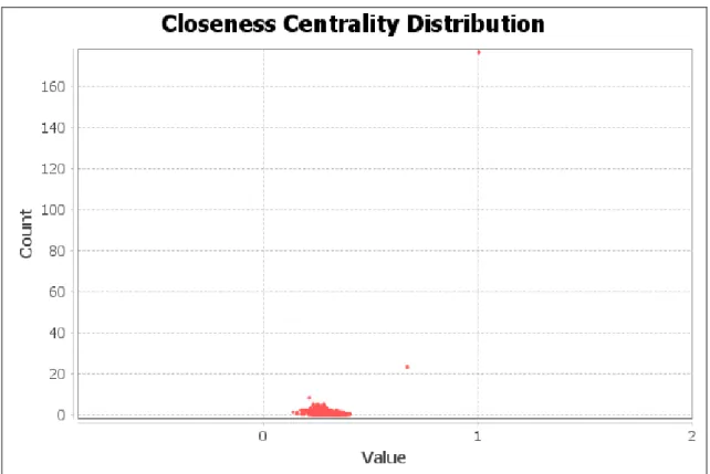
Figure 3.14 Closeness Centrality Distribution ... 23

Figure 3.15 - Eigenvector Centrality Distribution ... 24

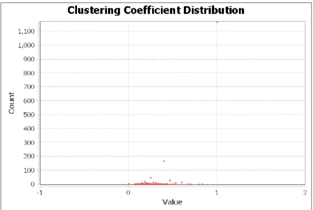
Figure 3.16 - Clustering Coefficient Distribution ... 24

Figure 3.17 - Nodes Table Network Measures Were Added ... 25

Figure 3.18 - Appearance Ranking Color ... 26

Figure 3.19 - Colored Graph ... 26

Figure 3.20 - Appearance Ranking Size ... 27

Figure 3.21 - Graph with size adjustments... 27

Figure 3.22 - Force Atlas Details ... 29

Figure 3.23 - Force Atlas First Graph ... 30

Figure 3.24 - Labeled Overlapping Graph ... 31

Figure 3.25 - Noverlap Settings ... 31

Figure 3.26 - Label Adjust Settings... 32

Figure 3.27 - Final Graph ... 32

Figure 4.1 – Degree Frequency ... 34

Figure 4.2 – Degree / other centralities for the entire network ... 35

Figure 4.3 – Degree vs other centralities for the top three percent ... 35

Figure 4.4 – Closeness Centrality ... 36

Figure 4.5 - Second Tier Connected to Giants ... 38

Figure 4.6 - Second Tier Connected via Average Nodes ... 38

Figure 4.7 - Third Tier ... 40

Figure 4.8 - Third Tier Close Up ... 40

Figure 4.9 - Aamir Khan Neighbors ... 42

Figure 4.10 - Shah Rukh Khan Neighbors ... 42

Figure 4.11 - Boman Irani Neighbors ... 43

Figure 4.12 – Akshay Kumar’s connections at the beginning ... 45

Figure 4.13 – Akshay Kumar’s connections after four years ... 45

(13)

1

1. INTRODUCTION

Movies provide an escape from reality to all cinema goers around the world. Ever since Thomas Edison invented the kinetoscope, the screens around the world have been providing entertainment to masses. Over time, the simplistic picture shows have evolved into a fully operational, revenue generating industries. These industries were localized to small communities at first but some of them have gained an enormous amount of international success and became art forms in themselves. An example of such an industry is the French cinema. Nowadays, whenever French cinema is mentioned, what comes to mind is a specific style of film featuring long shots and slow pace, wrapped in themes of existentialism and irony. The biggest of these globalized industries are Hollywood and Bollywood. Aside from providing financial security and jobs to thousands and thousands of people, they have also been a point of interest for researchers from all disciplines, including network analysis.

Network analysis is the scientific field of analyzing networks of all kinds. It has its roots in technology but over the past couple of decades, the mathematical disciplines have also taken up an interest in network analysis. Even though network science is relatively young as a field, its impact is of huge significance on both societal and scientific levels. Due to its enabling nature, the field of network science has become a subject of interest in the scientific research, companies rely on it to model their business, and it has even made its way into art and cinema.

This thesis is a case study of Bollywood from a network and data science perspective. The motivation for the study came from a personal interest in Bollywood and a passion for patterns and figuring out how things connect to each other. Bollywood is known to be colorfully chaotic and messy, thus, constructing a network model to represent it provides a better understanding of how Bollywood functions with respect to its players. The aim is to construct the actor network in Bollywood, analyze and investigate the resulting network, and explore whether the world-renowned actors of Bollywood are in

(14)

2

fact as powerful as they seem. To do this, the study investigates the network using the degree centrality measure to determine the well-known players according to their centralities, i.e. the study examines the fame through the number of people a person in the network has come in touch with, namely the people a person knows or how many people know them representing their fame.

The outline of the study is as follows: background information and literature review will be presented in chapter 2, including some theoretical framework. In Chapter 3, the software, data preparation and visualization will be described. Lastly, Chapter 4 will cover the analysis of the visualized data and the findings will be discussed.

(15)

3

2. LITERATURE REVIEW AND FRAMEWORK

2.1 Bollywood And Its Business Model

Bollywood is the first thing that comes to mind when people think about India. The term Bollywood specifically describes the Hindi-speaking aspect of the modern Indian cinema industry (Dwyer, 2010). Even though the industry, located in Mumbai, produces only the 20 percent of the total film output in all of India, it is the most widely known and appreciated subsection of Indian cinema with its international reach. The distinct style of Bollywood with its flamboyance and memorable dance numbers has given it the status of an international sensation (Ganti, 2004). Until receiving official recognition from the Indian government, Bollywood was mostly dominated by certain families (such as the Kapoors) which were treated as royals. All the decisions ranging from production to screening were made by these individuals. Following the formal recognition and partial funding from the Indian government, the industry began to change and aimed to follow a more professional business model in their ventures, upgrading their establishments to a Hollywood-based model, eventually reaching to audiences of millions across six continents. (Barat, 2018)

An organization/industry can spread and evolve in two separate ways: horizontal integration and vertical integration. Horizontal integration of an industry implies the outward expansion of the industry in various dimensions like production, distribution, marketing etc. and growing in size The latter, vertical integration, refers to a joint activity in different dimensions, e.g. distributors also having a say in the production of a movie. The model seen in Bollywood is an amalgamation of these two integration types: business groups. These business groups are an assembly of separate but managerially related firms (which then turn into clans) and the entry to the group is based on personal kinship to the firm (Lorenzen and Täube, 2008). Business grouping is vertical since the separate firms pool their resources and share the costs and revenue like a joint operation but also horizontal since they expand their size in time. This model is very fitting for Bollywood, an industry still in transition from the royal family model to a sustainable, more global business model. As the Bollywood’s business

(16)

4

model is still highly based on an actor/director/producers’ connections and kinship to others in the industry, it is a notable example to study from a network analysis perspective.

In this study, the focus is on actors’ connections to others via movies, so it is best to look at some of the key figures in Bollywood. One of the biggest household names is Aamir Khan whose films are almost always box office hits. Born in 1965 as the son of the producer Tahir Hussain Khan, Aamir’s reputation spans across the globe. Another reputable actor in the industry is Shah Rukh Khan who is sometimes referred to as King of Bollywood. Shah Rukh’s case is an exception to the norm as he didn’t have any family or friend connections in Bollywood prior to fame and he built up his stardom from scratch (Ganti, 2004) There is also a third Khan in the list of Bollywood’s most famous actors, Salman Khan who comes from a rich cinematic background and is very popular with the action genre fans (Salman Khan : Biography, Life Story, Career,

Awards and Achievements, no date). Among the famous actresses, names like Kareena

Kapoor, Kajol, Priyanka Chopra, Deepika Padukone can be found (‘Top 10 Most Famous Indian Actresses’, no date). These are only some of the big household names in Bollywood which also include but are not limited to: Sanjay Dutt, Amitabh Bachchan, Abhishek Bachchan, Boman Irani, Jackie Shroff, Sonam Kapoor, Akshay Kumar, Karisma Kapoor etc. Later in section 4, relationships among these actors and their co-stars will be examined more closely.

2.2 Graphs

A graph is a diagram that models the connections between a group of objects. These objects are called nodes (or vertices) and each line that connects the two nodes are called edges or links. Edges can be either directed or undirected. A directed edge implies that the direction the relationship has between two nodes plays a vital role whereas an undirected edge only connects the nodes and the direction of the connection has no importance. The graphs are named according to the types of edges they contain, e.g. if a graph comprises of directed edges, it is called a directed graph (Easley and Kleinberg, 2010). In Figure 2.1, an undirected graph with three nodes and three edges is shown.

(17)

5

Figure 2.0.1 - A Simple Graph

Various other forms of graphs exist. A graph is said to be weighted when the edges have real values assigned to them. Simple graphs contain no loops (i.e. a node having an edge with itself) and only one edge exists between two nodes. Graphs can also take on names according to the connectivity of their nodes. Two nodes are said to be connected if there exists a path between them. If every pair in a graph is connected, the graph is called

connected, otherwise disconnected. Another type of graph is a regular graph. If all the

nodes have the same number of neighbors, the graph is a regular graph. (Kadry, Seifedine, Al-Taie, 2018) A clique is defined by Bron and Kerbosch as the subgraphs within a graph where every node is adjacent to every other and the subgraph is not contained in another subgraph (Bron and Kerbosch, 1973).

Some basic concepts of graph theory must also be mentioned before delving deeper into graphs as network analysis visualizations. Centrality is a measure which expresses the importance of a node. By looking at the centrality of a node, the power the node holds over the network can be measured (Kolaczyk and Csárdi, 2014). Undoubtedly, the meaning of important varies from one situation to another. In real life relationship networks, having financial prestige might be the definition of importance for some; but for others, the number of friends they have might be what makes them central. Since graphs are powerful tools to model real-life networks and follow the same principles, the definition for centrality has been debated over the years. Even though a commonly and widely accepted definition does not exist, there are four classic centrality measures

(18)

6

used in graph theory and network analysis: degree centrality, closeness centrality,

betweenness centrality and eigenvector centrality.

Degree represents the number of adjacent nodes of a single node (Voloshin, 2009).

Following that logic, degree centrality implies the more neighbors a node has the more central it is. This simple measure is quite valuable in determining centrality in social networks: the number of connections a person has makes them more visible and central. In directed graphs, the in-degree (incoming edges) and the out-degree (outgoing edges) centralities can also be taken into account (Vasudev, 2006). Closeness centrality adds onto the degree centrality by considering the distance between a node and its neighbors: if a node is close to many others, it is considered to be central. When a node is on a path between two others, the importance of the said node is expressed with betweenness

centrality. The last classic centrality measure discussed in this study differs from the

previously explained ones. Eigenvector centrality indicates that the importance of one node depends on the importance of its neighbors, approximating the sum their centralities (Kolaczyk and Csárdi, 2014).

When dealing with graphs, it is also natural to consider its connectivity, i.e. if every single node can access every other node by a path. A path is a series of vertices such that every vertex in the series is sequentially connected to each other by an edge (Easley and Kleinberg, 2010) Paths are used to determine how information flows within a network and connectivity plays a key role in the flow. As mentioned before, a graph is called connected if there exists a path between all the nodes. However, most graphs that model real-life situations are not connected. These disconnected graphs consist of

connected components (or components for short): subsets that are have no paths to the

rest of the graph but are internally connected. If a connected component contains a substantial fraction of all nodes, it is said to be a giant component (Easley and Kleinberg, 2010). Bridges are the links in a graph so that if they were removed, i.e. cut, they would disconnect the graph and thus increase the number of connected components within the graph (Barabási, 2016).

(19)

7

Graphs can also be categorized according to how they are partitioned. A k-partite graph can be divided into k sets such that no node within the same set are adjacent. A bipartite graph is a k-partite graph where k=2. Likewise, when k=3, the graph is said to be tripartite (Cheng et al., 2007). The number of sets the data can be partitioned into depends on the nature of the data and the question explored. This number also defines the projections that can be generated from the graph.

Graph theory as a scientific branch dates back to 1700s with the solution Euler proposed to The Bridges of Köningberg problem. By representing each patch of land as a node and the seven bridges as edges, he paved the way to graph theory, by solving a problem with graph construction and showed that representing a problem as a graph can simplify and assist with the solution (Barabási, 2016). Ranging from airline routes to electrical grids of cities, all networks encountered in the physical world can now be mapped out as a graph to solve related issues and problems. Understanding graphs and graph theory facilitates the quantitative analysis of networks and leads to a clearer comprehension (Kastelle and Steen, 2010). Hence, graphs are a crucial element in network analysis of which the history and the basic principles will be discussed in the following section.

2.3 Network Analysis Basics

Dictionaries offer several meanings for the word “network” depending on the context it is used in. Cambridge English Dictionary has the most comprehensive definition for the word: “a large system consisting of many similar parts that are connected together to allow movement or communication between or along the parts” (network Meaning in

the Cambridge English Dictionary). This definition agrees with the idea that any system

can be viewed as network. With the development of technology and science research, networks were integrated into solutions for problems in other fields, including but not limited to transportation, medicine, sociology. Network analysis has become fundamental to the analysis of complex systems such as information networks, following the progress made in computer science and engineering fields in 2000s and later. The social media frenzy and its vast data size has particularly made network analysis a popular discipline (Kolaczyk and Csárdi, 2014).

(20)

8

While other disciplines treat a dyadic relationship as their base of analysis, network analysis demands a wholesome exploration of the entire group since every node in a network might indirectly affect the rest. Another principle followed is that the structure of a network is non-random. Due to transitivity and finite limits of connections, members (represented as nodes) of a network tend to cluster with the nodes they are causally linked with. Network analysts examine the outcomes of the linkage between these clusters (Wellman, 1983).

Network analysis principles and ideas are mostly based on graphs and graph theory – as mentioned in Section 2.3 – in the same way that differential equations are the foundation of mechanics. Most of the terminology is used interchangeably. Network analysis builds on the theoretical groundwork laid by graph theory (Butts, 2008). The partitioning is used widely in network analysis. A k-partite network can be modeled where k is defined by the problem. For instance, the human disease network is a bipartite network where each disease is connected to the gene with mutations that cause the disease. This disease network has two projections: one is a disease projection where diseases are connected if they share a common gene mutation cause. The other one is the gene projection where genes are connected if they are associated with the same disease. Should the data allow it, the human disease network can be expanded into a tripartite graph by including symptoms as another set of nodes. As mentioned before, the number k is defined by the research question and available data (Barabási, 2016).

There are three different approaches to a network analysis: descriptive analysis, modeling, and network processes. Descriptive analysis denotes the visualization of structures and creating numerical summaries of the data as a network. Modeling, however, seeks the answer to how network structures take their final form. Network processes approach focuses on the dynamic, ever-changing flow of network information (Kolaczyk and Csárdi, 2014). All these methods treat networks as a whole; changes in the domain do not have an independent effect on nodes; they are all affected. The wholeness of change is caused by the relational perspective, that is to say in network analysis, relations – rather than individual attributes of nodes – are the focal point (Marin and Wellman, 2009).

(21)

9

The data for the network to examine can be obtained through different channels using different methods. Surveys and questionnaires, while slightly dated, are still reliable methods. However, because of the progress of technology and the Internet, nowadays most of the data is available online. Archival data, social platform data, and even survey data can be accessed on various online platforms (Kadry, Seifedine, Al-Taie, 2018). Data available online is the easiest to access. However, it is best to keep in mind the data retrieved online could be prone to errors and missing values despite its accessibility. Even the most extensive data can contain inaccuracies, thus preprocessing the data as a first step is good practice.

2.4 Network Analysis Applications

Even though social sciences are the first to come to mind, many other research areas benefit from network analysis as a tool. One of the first signs of network concepts used in research was in the study of immigration in urban mass society by William Kornhauser in which Kornhauser studied the ties of immigrants to their ancestral communities (Wellman, 1983). Since then, network science has been spotted in various other research areas itself. Such an example area is ethnographic and nature studies: Hodder and Mol studied dependencies between humans and the things they own using centrality measures and a benefit-cost ratio respective to the entanglement, with the data obtained from Çatalhöyük archeological sites (Hodder and Mol, 2016). One study compares home-birth to other birth options by plotting out the care networks in each, i.e. by examining how far can a person reach in case they need to receive care (Andina-Diaz et al., 2018). Deng et al. examine the intergroup associations of Mongolian gerbils at during the food hoarding and mating season by creating a network of associations, demonstrating that Mongolian gerbils adapt their associations accordingly to balance the costs and benefits of survival and reproduction (Deng, Liu and Wang, 2017). Other examples of network analysis in other disciplines include but are not limited to a citation network of higher education (Calma and Davies, 2017), literary history (Long and So, 2012), diabetes in communities (Raghavan et al., 2016), job history as a risk factor in prostate cancer cases. (Dombi, Rosbolt and Severson, 2010), and brand positioning in marketing (Wang, 2015).

(22)

10

Perhaps the biggest area of interest in network science nowadays is the online social networks. Following the inception of platforms like Twitter, Facebook, etc., many researchers took an interest in these platforms as networks and their vast data. Mehrotra et al. proposed a method for detection of fake Twitter users by classifying the data according to their centralities (Mehrotra, Sarreddy and Singh, 2016). Similarly Hussain and Islam have explored whether or not tweet accuracy could be classified using centralities of each term in a tweet (Hussain and Islam, 2016). A study conducted in Turkey on social media usage in education has analyzed Facebook data to determine if Open Education students benefit from social media pages in their studies (Fırat et al., 2017)

Another topic that has sparked curiosity as a research area is the movies and their related data. Some researchers have explored through Twitter data to estimate the public’s response to new and upcoming movies (Lipizzi, Iandoli and Marquez, 2016) or to mine opinions of users by crawling through Twitter, collecting tweets and dissecting the opinions for understanding the customer sentimentality and behavior (Hodeghatta, 2013), or to mine the metadata to create a prediction scheme for the performance of movies (Kim et al., 2013). While online platforms constitute an interaction network for cinema industry, movies and their cast listings are networks in themselves. The famous saying “art imitates life” holds true in this case as well. The silver screen encompasses many types of associations: character-character, actor-actor, actor-director and so on, just as in reality. Tran and Jung have developed a method for extracting the character networks – which they dubbed as “CoCharNet” – using total screen time of characters and co-occurrences of characters (Tran and Jung, 2015). Yeh et al. have built on their previous research of automatic network construction by using cues from editing (Yeh, Tseng and Wu, 2012) to cluster faces in a film, aiming to approximate their relationships (Yeh and Wu, 2014). Packard et al. discussed the role of actors’ embeddedness in their networks as a factor of success in business (Packard et al., 2016).

Alas, most of the research is based on Hollywood. Bollywood as a data source in the network disciplines is still a matter open to exploration. Like Lipizzi et al.’s study,

(23)

11

Gaikar et al. used Twitter data to predict Bollywood movie performance by applying a fuzzy inference method (Gaikar, Marakarkandy and Dasgupta, 2015). One research has focused solely on Bollywood as a network of individuals to study the factors for network robustness by combining complex network theory and random matrix theory (Jalan et al., 2014). Even though the lack of Bollywood-focused research might seem disheartening, it implies that there are numerous opportunities for inquiry and investigation.

In the next chapter, details on the software utilized and data processes will be given, and the algorithms used will be discussed.

(24)

12

3. SOFTWARE AND DATA

3.1 Software Used

Network analysts and those who are interested in the subject can benefit from many tools. These tools come in a variety of forms and types; open source, commercialized, freeware, so on and so forth. Data processing, statistical and visualization tools are widely available for use. In this study, the preferred tools were open source for the sake of availability and easy usage: OpenRefine and Gephi, the former for data processing, and the latter for statistics and visualization.

3.1.1 OpenRefine

OpenRefine, previously known as Google Refine, is a powerful open source data clean-up and transformation tool. It first came into existence as Freebase Gridworks, originally intended as a supporting program for Freebase databases, created by Metaweb Technologies. Google acquired Metaweb Technologies in 2010 and the tool lived on as Google Refine until Google decided to discontinue support operations for the software in 2012. Following the end of Google branding, the name of the product became OpenRefine. It is currently available as a community support project on GitHub (Metaweb Technologies, no date).

3.1.2 Gephi

Gephi is a free open source tool for network analysis and visualization. Distributed under GPL 3, Gephi allows its users to visualize and manipulate networks and has some statistical capabilities. It has built-in exploration, analysis, visualization, and clustering functionalities among many others. It is written in Java which allows the developers to build on and improve Gephi easily (Gephi.org, 2018). A French non-profit organization called The Gephi Consortium oversees the improvements and future release developments since its inception in 2010. Gephi is used widely by academia, journalism, and anyone else who is a network analysis enthusiast (Wikipedia.org, 2018).

(25)

13

The free nature and the ease of use of Gephi has made a suitable choice of software for this study.

3.2 Data

India has a rich history of movies, spanning over 100 years, with different movie industries operating in Hindi, Tamil, Telugu, and various other languages. For this study, movies following the recognition and support from Indian government have been considered, as post-2000 Bollywood follows a more formalized business style. The data has been obtained from imdb.com and the missing values have been completed mainly via bollywoodmdb.com and other Bollywood related websites.

3.2.1 Preprocessing and form

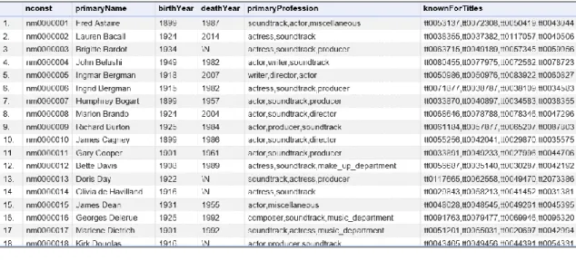
IMDb offers its data publicly on https://www.imdb.com/interfaces/ for non-commercial use (IMDb, 2007). The data can be directly downloaded from the website. It comes in compressed (.gz) format and includes a tab separated file (.tsv) with the same name. There are 6 different datasets utilized in this study: akas, basics, crew, episode, principals, and names.

 Akas: This file contains movies’ title, region, language, and type information.  Basics: This file has more detailed information on movies such as genre, runtime,

year etc.

 Crew: The crew file contains information on directors and writers.

 Episode: This file comprises of TV series season and episode information.  Principals: The principal file consists of the main cast and crew information.  Names: This file has the information regarding the people, such as actors, writers,

directors etc.

After the data had been acquired, it was time to clean up the messy, scattered data into one usable form. Since the datasets were too large to handle regularly with Excel or basic tools, OpenRefine was used. OpenRefine runs on the user’s computer as a small-scale local server and can handle large datasets with ease. One key step before doing

(26)

14

any operation on OpenRefine is making sure the allocated memory will suffice for handling the size of the data. Unfortunately, the .exe file does not allow custom memory allocation, but the user can by-pass this control measure by editing the configuration file and running OpenRefine from the batch file. Besides the memory parameter, the user can update the port, host, and other parameters according to their needs. In this study, both 8 gigabytes and 12 gigabytes of memory allocation were employed, depending on the file size which ranged from 80 megabytes to 1 gigabyte. The configuration file is shown below:

Figure 3.1 - OpenRefine Configuration File

The three main files necessary for this study were basics, names, principles, and akas files. Albeit scattered, they included all the necessary information for this study.

(27)

15

Figure 3.3 - Sample View of Names

Figure 3.4 - Sample View of Principles

(28)

16

Figure 3.6 - Sample View of Episode

As seen on the sample views, akas file included the language and region. From there, language and region were used to filter the Hindi movies released in India. Since the data includes all releases for one movie, the duplicates were removed to avoid unnecessary information and to reduce the size as much as possible to a manageable size. The “titleId” attribute is the unique id number for a movie and it acts like the reference attribute that led to the needed information in other files similar to a database primary key. The original list included all the available movies in Bollywood involving those from the pre-2000 “clan” era. To filter out the post-2000 movies, dates were collected from basics using titleId as key; the tconst attribute in basics was matched to the titleId. However, the TV series needed to be cleaned up too and the Episode set came to the rescue. The Episode data set included episodes of TV series and contained episode name, tv show name, episode number and season number. Anything in the

episode data set was removed by matching the titleId to parentTconst. The unnecessary

columns were eliminated from the remaining list of titles, which shall be named the

(29)

17

The names file contains the primary name of actors and each name has a unique identifier that acts like the primary key for names. By using these two distinct identifiers, names were matched to the titles they appeared in the principles. Then the titles not in our main movie list were marked and removed from the principles set, followed by the elimination of all categories except “actor” and “actress”. Even though the data included gender specification listing as actor and actress, gender was not taken into account in this study. The elimination process resulted in a list of names with the associated movie name, which shall be mentioned as main names list from this point on.

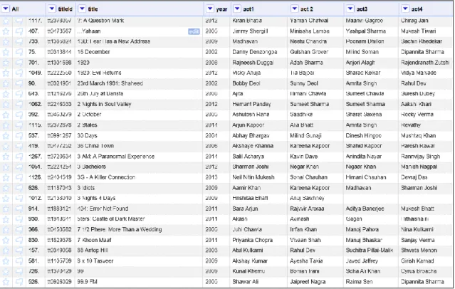
The following steps of the data preprocessing was unfortunately a bit of a manual work. Since a movie can have a considerable number of cast listings, only the first four actors were chosen to be in the network for suitability and ease purposes. Using filters on the main names list, each movie title was selected from the list and the four actors were added to the main movie list. While this process took more time than other automated missing value handling processes, it allowed for a simpler missing value elimination process and a closer control on the values. There were some instances where no actor data was available for a movie or only one actor was listed. These cases brought no advantage, thus were deemed ineffectual, and were removed from the data. Finally, the release year of the movies were added to the main movie list.

(30)

18

Figure 3.7 - Data After Missing Value Handling

In this study, cast members were chosen to be nodes and the movies they were in together were used as edges. Each node represents a unique actor and each movie is an edge. Each node had a node identification number (id) and the list of actors with ids constituted the nodes table. Creating an edge table for Gephi required coupling each actor with their co-stars, a combination in pairs, and adding the movie name as the edge label. Space characters in actor names between first and last names were deleted to avoid accidental duplication of nodes. For instance, in “3 Idiots”, Aamir Khan stars alongside Kareena Kapoor and Sharman Joshi. One row in the edge table had Aamir Khan as the source node and Kareena Kapoor as the target node to imply their relationship via 3 Idiots. Aamir Khan (source) and Sharman Joshi (target) were listed in the next row. Since the relationship between actors is always reciprocal, the edges were undirected, and no duplicates existed, i.e. no rows existed where Kareena Kapoor was the source and Aamir Khan was the target for the movie “3 Idiots”. Finally, for source and target node values, the node ids were employed rather than names for precision purposes.

(31)

19

Figure 3.8 - Nodes on Gephi

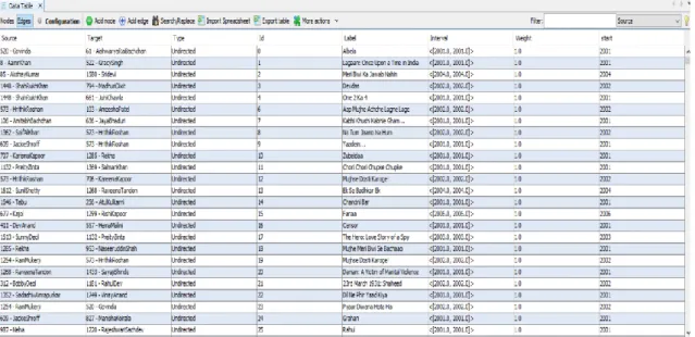
Figure 3.9 Edges on Gephi

(32)

20

Figure 3.10 – Node example with edges

As mentioned before, each node in Figure 3.10 represents an actor who has played a part, regardless of the scope of the role, in a movie. An edge between two nodes represents the fact that the two nodes have been in a movie together, i.e. they have worked together and know each other. The edges between nodes are undirected and unweighted based on the point of view that once these people work together, they are assumed to know each other. In other words, simply the existence of a relationship between two people, constitutes the edges. Taking Figure 3.10 as an example, Nafisa Ali and Sabyasachi Chakraborty know each other through work and their relationship in the film “Lahore” creates an edge. To sum it up, this study uses a unipartite simple graph as a network model with nodes as actors and films as unweighted and undirected edges, partially due to the data constraints and the fact that our aim is to see the well-known players using mainly their degree centrality, i.e. how many connections they have within the network. The nodes, due to faults in data and various computation issues, have no attributes such as gender, birth date, height, weight, ethnic background

(33)

21

and et cetera. Moreover, our data could have been modelled as a bipartite graph with two sets of nodes; one set of nodes as actors and the other as movies. However due to the limitations imposed by the data’s nature and the requirement for manual data validation and missing value handling, network examined in this study was constructed as unipartite. To explore the effect of time on the connection between nodes, the release year was employed to enable the timeline function.

3.2.2 Visualization

After finalizing the tables, the data was imported into Gephi using the import spreadsheet functionality in the data laboratory. There were 1814 nodes and 7622 edges. At first glance, the graph seemed like a mess: dark, similar-sized nodes with edges overlapping each other and creating a jumbled mess. To make sense of and turn it into an analyzable network model, the application of some visualization operations was necessary on the raw data.

(34)

22

Before moving any further with visualization, the tests provided by Gephi were run. These tests computed the essential network measures such as degree, eigenvector centrality, average path length and so on and so forth. The tests come as built-in functions with Gephi. After each test, the related information was added as an attribute to the nodes in the data laboratory tab in Gephi. The implication of these network measures shall be discussed in Section 4 but for the preliminary results of the tests and automated graphical presentations are as detailed below:

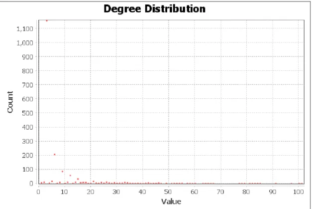
Figure 3.12 - Degree Distribution

(35)

23

Figure 3.13 - Betweenness Centrality Distribution

(36)

24

Figure 3.15 - Eigenvector Centrality Distribution

(37)

25

Network Measures Result

Nodes 1814

Edges 7622

Average Degree 7.712

Network Diameter 10

Average Path Length 3.810

Average Clustering Coefficient 0.750

Table 1 - Summary of Network Analysis Measures for the Network

Gephi adds the results for every node automatically to the nodes table as attributes so that the users can see the values easily for each of them while analyzing the network. These values are added as columns automatically, each column represents one result. The results for this study in the nodes table came out as sampled below:

Figure 3.17 - Nodes Table Network Measures Were Added

At this point the values were added but the graph itself was still a mess. The appearance of the graph had to be improved before any layout application. Gephi has a built-in appearance function that provides support for ranking based appearance option. Among the many choices offered, degree centrality appeared to be a fit choice for this study’s purposes. The higher degree indicated that the actor had more connections and was more well-known within the network. The color scheme was from red to blue; those with lower degree centrality were red nodes and those with higher degrees were blue.

(38)

26

Figure 3.18 - Appearance Ranking Color

(39)

27

The same procedure was followed for size. Using degree centrality, nodes were resized ranging from 20 to 200.

Figure 3.20 - Appearance Ranking Size

(40)

28

The color and size of the nodes were fine-tuned according to their degree centrality. However, that process made no improvements to the general form and the graph was mostly unintelligible. The practical layout tool of Gephi was used to improve the look and visibility of this cluttered graph. Fortunately, the built-in layout feature in Gephi offers a variety of layout options. A few of them could be used in this study.

Fruchterman-Reingold layout operates on the idea of attraction/repulsion, but it creates a model where nodes are treated as mass particles with edges as springs between them. While it is widely used, it is quite slow with the complexity of O(N2_).

Another renowned layout in Gephi is the Yifan-Hu layouts (regular and proportional) developed by Yifan Hu. It is akin to other force-directed layouts with one small difference: it approximates the force of a cluster on a distant node, handling the cluster as one super node.

The ForceAtlas and ForceAtlas 2 algorithms are based on attraction/repulsion strength. Force Atlas groups similar nodes together and drives apart the dissimilar ones. Force Atlas 2 works on the same principle; however, the algorithm complexity is reduced by replacing two parameters with just one “scaling” parameters. Force Atlas and Force Atlas 2 is a suitable layout option for real world scale-free networks. The difference between the two types of the Force Atlas layouts is that Force Atlas 2 allows more layout options and allows the user to control speed and performance more freely than the original Force Atlas algorithm. Since Force Atlas 2 is a more suitable option for larger networks and our data is relatively small in size compared to other networks such as the human disease network, the original Force Atlas algorithm suffices for our purposes.

There is one other neat layout which is used after applying regular layouts: Noverlap. Noverlap layout – as the name suggests “no overlap”– prevents nodes from overlapping without affecting the shape of the graph. Among these layouts, ForceAtlas and Noverlap were used in this study for clarity and speed reasons. ForceAtlas’ “attraction distribution” setting was checked to push the hubs to the outer edges for a more

(41)

29

comprehensible graph. This is purely a styling choice; a user can prefer to see the hub nodes in the center rather than the outer lining. Since the focus of this study is determining the well-known players in the Bollywood game, aligning the hubs on the outer boundary of the graph provided clarity. The gravity was set to 30 to keep any of the components from drifting too far away from the central elements. Adjust by sizes option was used despite the fact that this option causes an increase in the runtime of the algorithm. First the Force Atlas was run on the graph. ForceAtlas took about twenty minutes to complete and resulted in the graph given below with the following settings specified:

(42)

30

Figure 3.23 - Force Atlas First Graph

At this point, the graph did not require Noverlap to be applied yet since the node locations were adjusted by the respective node size; there was enough space between nodes. Next step to improve visualization is to add the node labels to know who the hubs and outliers are. The labels made the graph more informative at the first glance; however, the graph was a huge mess with the labels entangling and crossing over each other. It was quite hard to read and needed simplification. The Noverlap algorithm and the Label Adjust algorithm were run to prevent labels overlapping and cause confusion. Following this step, the network graph took its final form.

(43)

31

Figure 3.24 - Labeled Overlapping Graph

(44)

32

Figure 3.26 - Label Adjust Settings

(45)

33

4. ANALYSIS AND FINDINGS

Now that the preparation of the graph has been explained, the time to delve deeper into the network created from the Bollywood data has finally come. In this chapter, the structure and implications of the structure will be discussed.

In the previous sections, the term “hub” was used in its general sense, to explain the general workings of algorithms and how they functioned within the scope of the Bollywood data. However, from this point on, the term hub will refer to the top three percent of the nodes according to their degree centralities. In Section 3.2.2 Visualization, the summary of network measures was provided as a table. As shown in the table, the average degree of the network is close to 8 and the clustering coefficient of this model is 0.75. Such a high number of clustering and average degree can be expected from an industry where whom you know matters despite the changes in the business model. As mentioned before, this model takes degree centrality into account as a measurement of “importance” or the identifiability of the well-known players. The degree centrality in the network represents how many people one person knows within the modeled network or how many people know a person since the relationship between these players are reciprocal. The degree range of the nodes in this model ranges from 0 to 101, with the average being 7.712. In Figure 4.1 below, it’s seen that the degree distribution is highly asymmetric and most of the nodes have lower degrees. This shows that the network is mostly resilient to failures, i.e. random removal of nodes such as the death of an actor, since the randomly chosen node will most likely have a lower degree.

(46)

34

Figure 4.1 – Degree Frequency

One might wonder why degree centrality alone was chosen to define what a well-known player is within this network. In some cases, the degree centrality might be ineffective to explain the significance of a network. Other centralities such as betweenness and eigenvector centralities are used in other cases depending on what’s being looked at. One might look at the information flow of a network and choose betweenness centrality to see which nodes control the flow of information and are vital in that sense. Sometimes who you are is not enough and whom you are connected to also matters, in that case, the eigenvector centrality is measured and chosen. In Figure 4.2 and 4.3 below the distributions of these centralities against the degree centrality are given. The centralities other than the degree have been normalized for precision purposes. We see that the higher the degree centrality, the higher the betweenness and eigenvector centrality. Aside from being “well-known”, namely having high degrees, these nodes also take on brokerage roles and make way for new connections for new movies to form. They also seem link together with other important nodes, resulting in high eigenvector centralities. Exceptions do also exist; Gulshan Grover who has a degree of 83 has a higher betweenness centrality than the top player Akshay Kumar in the

(47)

35

network. But generally speaking, hubs have higher centrality results than the smaller nodes which symbolizes their role as an intermediary between others.

Figure 4.2 – Degree / other centralities for the entire network

(48)

36

Another interesting exception to centrality measures here is the closeness centrality. Among the top three percent of nodes which were defined to be hubs, higher degree hubs are closer to all the other nodes within the network than the rest. This can be accepted as Bollywood network seems to be tightly packed. However, when the model is looked at as a whole, a few exceptions are witnessed. There are a few cases where the degree is extremely low, but the closeness is higher as seen in the first graphical representation in Figure 4.4 below. This happens when a node is tied to the key nodes directly or a node is in a connected component. When examined, the case in the Bollywood network is generally the latter. The nodes in the connected components seen on the outer edge have higher closeness centralities but they have low degrees due to the fact that the components they are in are relatively smaller in size as compared to the giant component of the network.

Figure 4.4 – Closeness Centrality

The shape of the graph looks a bit like a fish swimming down or perhaps a bait-ball which is the formation that small fish (e.g. sardines) gather into a swarm as a safeguard against threat. A tightly-knit giant cluster at the center is observed; the crisscrossing connections are packed together near the hubs, expanding from the hubs at the bottom

(49)

37

and the sides, dispersing out and upwards to the groups. The reason for this expansion from one side to the other is explained in Section 3.2.2 Visualization: the Force Atlas algorithm pushes the hubs to the outer edge for comprehension purposes when attraction distribution is applied. With Force Atlas the cascading nature of social connections is observed better than with other algorithms. For instance, while the Fruchterman-Reingold provides a clearer view of the hubs themselves, the layered nature is harder to observe.

There is a second tier of connections in the network. Sets of small clusters are linked to the main giant component via bridges. These bridges lead either directly to the hubs in the network or to a node with average degree at the edge of the network, connected to the main body through the average degree node. In Figure 4.5 Deb Mukherjee and Shivkumar Subramaniam are examples of the second-tier nodes connected directly to hubs, in their case the hub is Priyanka Chopra who is an influential node. The path length in this case is 1 – shorter than the average length of 3.81. Figure 4.6 showcases the nodes connected via an average node. Poonam Pandey which is an ineffectual node is linked to the main cluster through average nodes like Suzanna Mukherjee and Iris Maity. In this case, the shortest path length to the closest influential node Manoj Bajpayee is 6. Poonam Pandey has also a path length of 6 to one of the biggest hubs Amitabh Bachchan.

(50)

38

Figure 4.5 - Second Tier Connected to Giants

(51)

39

In Figure 4.7, a number of cliques can be observed on the periphery of the graph. This third level tier exists on the peripheral border where these cliques are small and disconnected from the graph. Most of these are made of four nodes with a few exceptions and they are completely separated from each other and the rest of the graph. The four elements in each may be attributed to the data processing methods since only the first four members of the cast were chosen. However, there are a couple of sets that consist of seven members and one that has only three nodes. In Figure 4.8, both exceptions to the four-member sets can be seen. On the left side, one of the seven-member sets are seen and on the right side, the circle of three is present. Previously in this section, nodes with high closeness centrality scores despite having low degrees were discussed. These cliques fulfill the condition of low degree-high closeness centrality. The degrees of the nodes are low since they are disconnected from the giant component and are only connected within, but they have a high closeness centrality since they are close to all the other nodes in their own clique.

This isn’t a rare occasion, almost all graphs have this kind of formation since cliques take form in real life too. One may choose to perceive these as outliers and remove them from the data, but in the context of networks and Bollywood, they create an interesting case. This formation might happen due to the nature of the films these actors have performed in: they may have chosen to star in independent films, thus, not reaching a larger audience and not capturing the eye of the casting directors who could have let them star along the bigger stars. Another reason that comes to mind is that these cliques might represent the films that have flopped in the box office and the actors lost their chance to enter the giant component via other movies. The specific reasons as to why such formation occurs in Bollywood need to be the subject of further examination, should some extra information be added to the data.

(52)

40

Figure 4.7 - Third Tier

(53)

41

When looking at the graph as a whole, it is seen that some nodes stand out compared to the others. For instance, Akshay Kumar, Amitabh Bachchan, Ajay Devgn, Anupam Kher, and Gulshan Grover are the first five that meets the eye. These all have degrees above eighty with Akshay having the highest degree of 101 and are within the top three percent. Surprisingly, the internationally celebrated actors such as Aamir Khan, Shah Rukh Khan, and Katrina Kaif have lesser degrees. For anyone who is a fan of Bollywood or at least is familiar with some aspects of the industry, such a result is counter-intuitive. However, from a perspective purely based on movies as connections, some explanations can be given for this occurrence. One of these explanations for this phenomenon could be the principle of selectivity which well-known actors use when choosing films; these actors choose their roles carefully to maximize their gain, whether it be personal or economic, and have to eliminate the movie offers which do not fit their already busy schedule. This principle of selectivity results in a smaller number of movies made, and therefore, fewer connections with other actors. |It also explains why supporting actors have higher degrees than renowned actors. Supporting actors take on more roles in the same period because of a less busy schedule and the nature of the roles; their parts in the films are smaller, so they spend less time on a project and can move on to another one while the lead actors have more scenes to shoot and have other engagements like film galas, award shows, advertisement deals, so on and so forth. A visual proof of this occurrence can be found in the graph. In Figure 4.9 and Figure 4.10, Aamir Khan’s and Shah Rukh Khan’s connections are given and in Figure 4.11 Boman Irani’s connections are shown. It is depicted that Boman Irani as a supporting actor has links to more actors than the two Khans. Despite being less famous in the international scene compared to the Khans, he is more well-known within the network of Bollywood.

(54)

42

Figure 4.9 - Aamir Khan Neighbors

(55)

43

Figure 4.11 - Boman Irani Neighbors

In Section 3.2.2 Visualization, the tests showed that the network diameter is 10 and the average path length between two nodes is 3.81. On average Bollywood network seems compatible with the theory of six degrees of separation proposed by Milgram (Travers and Milgram, 1969). While one could choose those nodes which are 10 distances apart, a random node would need to traverse across 4 nodes on average. The low average path length combined with the high clustering coefficient of 0.75 shows that Bollywood network is a small world network. Between the hubs, the shortest path length is at most two, e.g. Akshay Kumar and Emraan Hashmi connect via Mithun Chakraborty. Likewise, Gulshan Grover and Amitabh Bachchan have a path of one between them. A question that comes to mind is how the actors that are related in the real world connect with each other in the graph representation of the network. An example of such a relationship is the one between Kareena Kapoor and Ranbir Kapoor. Kareena and Ranbir are first cousins and the grandchildren of the legendary Raj Kapoor who is known best for his performance in “Awara Hoon”. One would expect the shortest path between the two cousins to have the distance of 1; however, the shortest path in our graph between Kareena and Ranbir is 2, the connection made via Deepika Padukone. This case is a fitting example of how Indian government’s funding and recognition has

(56)

44

changed Bollywood’s business model from the ruling clans to formalized business groups: before the government funding, one would expect Ranbir to play in the same movie as Kareena as back in the day when actors were most likely chosen from within family. Another case in which we see this change is the relationship between Aamir Khan and Imran Khan, the uncle and the nephew. Aamir and Imran have a path of distance 2 between them – with Boman Irani connecting them – despite being close relatives. However, there are instances of relatives being directly connected to each other, e.g. Abhishek Bachchan and his father Amitabh Bachchan. The same direct connection can be seen between Sunil Dutt and Sanjay Dutt. While Bollywood is changing its form and becoming more of an open competition for all, it cannot be reasonably assumed that this is the case for all families and there is still time for Bollywood to become a fully formalized industry.

Using the year information provided in the data, the timeline function was enabled and the change in an actor’s connections over the years was observed. Akshay Kumar, who has the highest degree in this network, can be used as an example with a two-year interval. The number of connections Akshay Kumar has increased at each passing interval. Such occurrences are reasonable and reflect the real world well since most actors become increasingly involved with the industry over the years, making more movies and costarring with more people – thus expanding their personal network as well as helping the network grow.

(57)

45

Figure 4.12 – Akshay Kumar’s connections at the beginning

(58)

46

Figure 4.14 – Akshay Kumar’s final set of connections

Ideally, in a dynamic network, the entrance and exit of nodes to the network should be observed. However, the data of this study had a lack of details in time format, i.e. only the year data was available, which prevented a comprehensive approach to be taken. Also, the birth and death years of the actors in the network have been lacking. Had the data structure allowed it, the network could have been constructed as a time series where the evolution of a node and its value can be observed through time.

(59)

47

5. CONCLUSION AND FUTURE WORK

This study originated from a mix of passion for Bollywood and an interest in networks and connectivity. Data from the world’s biggest database has been retrieved, cleaned, and arranged into a set of nodes and edges to depict a graph. Using graph visualization software, the network of Bollywood was analyzed. Using the degree centrality measures, the structure of the network, the cliques and the hubs, and the influence of nodes which correspond to the world-renowned actors have been discussed.

There are many possibilities for future work to be explored henceforth. To begin with, tools and languages more suitable for data analysis and statistical computing could be employed, such as the language R and RStudio. In addition, to overcome the problems in data validation, a software can be developed that will crawl the movie related websites and gather the data so that it would suit the needs of network analysis much better. Since only the necessary information would be collected, it would significantly decrease the time spent on preprocessing and would also allow for reducing the amount of manual data correction performed on the dataset.

As mentioned in Section 3.2.1, the limitations imposed by the by the data affected our network model heavily and the network had to be constructed as a unipartite network and simple graph. Correct data forms can override this issue so that creating more functional bipartite network models becomes a straightforward and improved process. Choosing a bipartite model has its advantages over the unipartite form; it offers a versatile and better view of a network from both projection sides and minimizes the information loss. Aside from the partitioning of the network, time can be factored in when analyzing Bollywood. Even though a time series view of the Bollywood network has been attempted, the aforementioned data limitations hindered the efforts to see how Bollywood and its members interacted with each other over time. Although some changes could be tracked with the current model in this study, there is still an opportunity for a more in-depth analysis in the future.

(60)

48

Similarly, the Bollywood data from the old era of Bollywood can be included. If the time frames are defined clearly, the changes in Bollywood network which came with each period can be examined and the structures of networks in these time frames can be compared with each other. For instance, Raj Kapoor’s era and his grandchildren’s era can be observed and scrutinized for similarities and difference in terms of business models and artistic changes.

There are many other things and ideas which would advance this case study into a higher level. Correlation analyses, using concepts of homophily and assortativity, are promising areas to expand to. Even though we can see somewhat of a degree assortativity (high degree nodes being associated with high degree ones and vice-verse) in this model, other kinds of assortativities and homophilies are opportunities for research. The age of an actor is a promising attribute. Since most real life human social networks show age homophily, people of the same age communicate more than different age groups. Age as an attribute would help determine whether age is a factor in casting in Bollywood. Another attribute which can be included is gender; this study has not taken gender into account but in the future, a gender studies perspective on a network like this can be taken. Other attributes that one might consider are the number of awards won, preferred genre, highest paid salary for a movie et cetera. These node attributes would provide insights on the nodes’ aspiration and conformity levels and act as a base for a business decision system. Multiplicative Attribute Graph model, proposed by Kim and Leskovec, considers the likelihood of an edge forming between two nodes and how assortativity affects the general structure of the network (Kim and Leskovec, 2011). Adding categorical node attributes to the current model to use MAG would allow it to capture connectivity patterns better and help understand Bollywood’s business better.

In Section 3.2.1, the reasons as to why this model wasn’t constructed as bipartite were explained and how it could have been so if it weren’t for the data constraints. Assuming the tools mentioned before such as the data crawler are built, a bipartite model with one actor node set and one movie node set would be advantageous. The movie nodes would have attributes such as running time, release year, genre, country, language, budget, and