KADIR HAS UNIVERSITY
GRADUATE SCHOOL OF SCIENCE AND ENGINEERING
GRADUATE THESIS
CHURN ANALYSIS AND PREDICTION WITH DECISION TREE AND
ARTIFICIAL NEURAL NETWORK
2
SAFA ÇİMENLİ
S afa Ç imen li M.S . T he si s 2015 S tude nt’s Ful l N ame P h.D. (or M.S . or M.A .) T he si s 20 11
CHURN ANALYSIS AND PREDICTION WITH DECISION TREE AND
ARTIFICIAL NEURAL NETWORK
SAFA ÇİMENLİ APPENDIX B
6
Submitted to the Graduate School of Science and Engineering In partial fulfillment of the requirements for the degree of
Master of Science In
COMPUTER ENGINEERING
KADIR HAS UNIVERSITY May,2015
2
ABSTRACT
CHURN ANALYSIS AND PREDICTION WITH DECISION TREE
AND NEURAL NETWORK
Safa Çimenli
Master of Science in Computer Engineering Advisor: Asst. Prof. Taner Arsan
May 2015
Nowadays market competition is increased in logistic sector. Retention of customers due to the competition has gained importance. Retention of customers is more advantageous than gaining new customers. Gaining new customer has 5 units more than retention of existing customer. Especially telecommunication companies use churn analyzing and prediction. However competition increased in different sectors and they need churn analysis. In recent years logistic companies increased in Turkey, so retention of customer and churn analysis are important for logistic companies. Some logistic companies have churn committees and work on customer loyalty. This article includes churn analysis and prediction with decision tree and artificial neural network. In addition, this article includes comparison of 2 different methods for churn analysis. Article results show neural network better than decision for prediction. Because decision tree churn prediction rate is %81, Artificial Neural Networks rate is 97%. AP
PE ND IX C
3
KARAR AĞAÇLARI VE YAPAY SİNİR AĞLARI KULLANILARAK KAYBEDİLEN MÜŞTERİLEN ANALİZİ VE TAHMİNİ
Safa Çimenli
Bilgisayar Münedisliği Ana Bilim Dalı Yüksek Lisans Danışman: Yard. Doç. Taner Arsan
Mayıs 2015
Özet
Günümüzde bir çok sektörde olduğu gibi lojistik sektöründe de rekabet artmıştır. Mevcut müşterileri ikna etmek ve elde tutmak da pazardaki rekabetde ayakta kalabilmek açısından önemini arttırmıştır. Mevcut bir müşteriyi elde tutmak yeni bir müşteri bulmaktan daha avantajlıdır. Çünkü firmalar mevcut müşterileri elde tutmak için 1 birim maliyet harcarken, yeni müşteri bulmak için 5 birim maliyet harcamaktadırlar.
Özellikle telekomunükasyon firmaları churn analizi ve tahmini yapmaktadırlar. Ayrıca rekabetin arttığı diğer sektörlerde churn analizine ihtiyaç duymaya başlamıştır. Türkiyedeki lojistik firmaların sayısı son yıllarda artmıştır. Dolayısıyle lojistik sektörü içinde churn yönetimi ve analizi önemli bir noktaya gelmiştir. Bazı firmalar churn için özel komiteler kurup özel olarak bu konuda çalışma yapmaktadırlar.
Bu çalışmada churn analizi ve tahmini 2 farklı yöntem kullanarak yapılmıştır. Bunlar yapay sinir ağları ve karar ağaçlarıdır.Ayrıca bu 2 farklı yöntem arasındaki kıyaslamada yapılmıştır. Elde edilen sonuçlar da görülmüştür ki yapay sinir ağları churn analizi ve tahmininde daha etkili sonuç vermektedir.Bunun en temel sonucu karar ağaçları 81% doğru tahmin yaparken, yapay sinir ağları 97 doğru sonuç vermektedir. AP PE ND IX C AP PE ND IX C
4
Acknowledgements
Firstly, I would like to thank my sincere gratitude to my advisor Asst. Prof. Dr. Taner Arsan, for his patience and immense knowledge.
As a same time I would like to thank Cem Çomak and Bahar Bilen. They are working in UPS Turkey marketing department. They helped me for marketing subjects. And thank Burak Köken. He is IT manager in UPS Turkey, he helped me for support data.
Thank Mr. Mustafa Acungil for helping me to understand churn analysis and prediction.
I would like to thank to Research Assistant Serkan Altuntaş. He is helping me during the whole period of my master study as the best classmate in my life.
And finally, I would like to thank to my family for their endless support. AP
PE ND IX C
5
Table of Contents
ABSTRACT... 2 Özet ... 3 Acknowledgements ... 4 List of Tables ... 8 List of Figures ... 9Churn Analysis and Management ... 10
1.1 Introduction ... 10
1.2 Decision Tree Algorithm ... 11
1.2.1 Root Nodes: ... 12 1.2.2 Chance Nodes: ... 12 1.2.3 End Nodes: ... 12 1.2.4 Impurity-based Criteria : ... 13 1.2.5 Information Gain: ... 13 1.2.6 Gini Index: ... 14
1.2.7 The likelihood ratio is defined as: ... 14
1.2.8 DKM Criterion: ... 14 1.2.9 Gain Ratio: ... 15 1.2.10 ID3: ... 15 1.2.11 C 4.5: ... 16 1.2.12 CHAID: ... 17 1.2.13 MARS: ... 18 1.2.14 QUEST: ... 19 1.2.15 CART: ... 19
6
1.3 Neural Network (NN) Based Approach ... 23
1.3.1 Input Layer: ... 23
1.3.2 Hidden Layer: ... 23
1.3.3 Output Layer: ... 23
1.3.4 Feed Forward Neural Network: ... 24
1.3.5 Feed Back Neural Network: ... 24
1.3.6 Structure of Artificial Neural Cells: ... 25
1.3.7 Inputs:... 26 1.3.8 Weights: ... 26 1.3.9 Collection Function: ... 26 1.3.10 Activation Function: ... 26 1.3.11 Cells Outputs: ... 27 2. Related Works ... 28 3 Material Methods ... 30
3.1 Customer Churn Data of UPS Turkey ... 30
3.2. Generated Decision Tree Model and Prediction with R programing ... 36
3.3 Generated Neural Network Model and Prediction with R programing ... 39
4. Result And Discussion ... 43
4.1 Decision True Churn Prediction Results ... 43
4.2 Artificial Neural Network Churn Prediction Results ... 44
4.3 Compare Decision Tree and Artificial Neural Network Churn Analysis: ... 45
CONCLUSION ... 46
7 APPENDIX B
8
List of Tables
Table 1.2.1.14 Classification Tree vs. Regression Tree……… 13
Table 2 Related Works...………...……… 19
Table 3 Sample Data ………... 31
Table 2.3 Data Set Summary ……… 24
Table 4.1 Decision Tree Prediction Rate …………...……… 13
9
List of Figures
Figure 1.2.12 Decision Tree CHAID Algorithm……… 17
Figure 1.2.14 Decision Tree QUEST Algorithm……….... 18
Figure 1.3.4 Artificial Neural Network Feed Forward Algorithm………. 23
Figure 2.2 Artificial Neural Network Churn Model Graphic………. 32
10
Churn Analysis and Management
1.1 Introduction
In recent years competition and the growth of the logistics sector increased in Turkey. When competition increased, logistic companies give importance to churn management and customer loyalty. Customer retention and loyalty means saving money for company. Because finding new customer cost 5 units more than the cost of retaining loyalty customer. In addition, valuable customer loss and change logistic company is important for market competition. So logistic companies focus on churn management or mentored from consultant firm. Some companies create churn committees in house in their own company.
Most of the time, logistic companies use sales report and feedback prepared by sales persons. However, it is not very useful and easy. Big data is more important in this area as other sectors for decision, strategic and financial situations. Companies use big data for churn analyzing and prediction. Churn analyzing is more difficult than telecommunication sector, because logistic companies have irregular and scattered data. Churn analyzing is analysis of lost customer and prediction of the probability of losing valuable customer. After the analysis process, companies work on retention of the loyalty customer.
In this article, we study an American logistic company which occupies a large part of the market and customers. We will be studying its customer data. This dataset includes different types of value and irregular data. For example, customer shipment record, customer payment record and lost and damage record, complaint record under the CRM system.
11
We can churn analysis with different data mining methods and algorithms. In this case, we examined Decision Tree and Artificial Neural Network. We found maximum prediction rate by two methods.
1.2 Decision Tree Algorithm
Decision tree is supported decision with processing in dataset. Also decision tree appear a tree. Tree is a predictive model. Decision tree is supported a decision. It uses a graphical tree-like. Also, it gives possible results as model of decision. Decision tree contains chance event outcomes, resource costs and utility. It shows as an algorithm. Decision trees are used for data mining, statistic , operational research , decision analysis unique decision analysis.
Decision trees can drawn by users hand. Otherwise, some graphics program and specialized software are used for drawn decision tree. For example, weka, clementine, sas. When a group are focused on a subject, for take a decision they use decision tree. It is helpful them. Decision tree is used monetary, time or other values which are to possible outcomes, it is supported make decision automated in programmatically. Decision tree software is used some business branches which are data mining, strategic challenges and evaluate the cost effectiveness of research and business decisions.
Further decision trees are produced by Decision trees consist with algorithms and they are defined different ways. Branch-like segments include splitting data. The segments from an inverted decision tree that originates with a root node at the top of tree. Node is symbol in decision tree. It is represented decision alternatives, chance outcomes or a branch terminated. Decision tree has 3 types of nodes.
12 1.2.1 Root Nodes:
It is not have incoming edges and zero or more outgoing edge. It is represented by squares. Classification pattern starts with root node. Assigned pattern in category of leaf node.
1.2.2 Chance Nodes:
Chance node is defined an event in decision tree where a degree of uncertainty exists. It has other name is chance event node. It is represented by circle.
1.2.3 End Nodes:
It is represented by triangle or uncertainty node. The end node represents a fixed value.
Discrete splitting functions has single variable. Single variable is defined internal node is split according to the value of a single feature.
These are:
According to the origin of the measure:
Information theory, dependence and distance.
13
Impurity based criteria, normalized impurity based criteria and binary criteria. I examined the most common criteria in literature.
These are ;
1.2.4 Impurity-based Criteria :
Given a random variable x with k discrete values, distributed according to P=(p1, p2, …pk) an impurity measure is a function.
i) φ (P) ≥ 0
ii) φ (P) is maximum if ∃ i such that component pi=1.
iii) φ (P) is symmetric with respect to component of P.
iv) φ (P) is smooth (differentiable everywhere) in its range.
1.2.5 Information Gain:
Information increase is an impurity-based principle that uses the entropy size (origin from information model) as the impurity size.
Information Gain (ai,S)=
Entropy (y,S)-∑ ( |σai=vi,j||S| )
vi,j∈dom(ai) . Entropy(y, σai = vi, jS)
14
Entropy(y,S)=∑ ( −|Gy=cjS||S| + log2|Gy=cjS||S| ) cj∈dom(y)
1.2.6 Gini Index:
Gini index is an impurity-based principle that measures the divergences between the possibility supplies of the target aspects values. The gini index been used in numerous Works. It is expressed as:
Gini(y,S)=1-∑ ( |σy=ys||S| ) ²
cj∈dom(y)
Subsequently the assessment benchmark for choosing the attribute ai is expressed as
GiniGain(ai,S)=Gini(y,S)− ∑ ( |σai=vi,jS||S| ) . Gini(y, Gain(vi, j, S)
vij∈dom(ai)
Likelihood-Ratio Chi Squared Statistics:
1.2.7 The likelihood ratio is defined as:
G² (ai,S)=2.ln(2).|S|. Information Gain|ai,S|
Attribute of the target is one temporary independent and the zero hypothesis is contribution direction. If H0 keep, the test statistic is deployed x² with the degrees of freedom equal to (dom(ai)-1).)dom(y-1).
15
It is used for binary class attributes. DKM Criteria is based on impurity and it is designed as a splitting criteria. It was found Dietterich. And updated by Kearns and Mansour.
The formula is the impurity-based:
DKM(y, S) = 2. sµ |σy= c1S| |S| · µ |σy=c2S| 1.2.9 Gain Ratio:
The gain ratio makes the information gain as standardized like that: GainRatio(ai,S)=InformationGain(ai,S)
Entropy(ai,s)
That mean, if the denominator is zero, so this relationship is not defined. At the same time, the ratio can tend to favor attributes when the denominator is small. Therefore, gain ratio shown as two phases. Firstly, information gain is computed with every aspects.
There are several decision tree algorithm. I examined them. These are ID3(Iterative Dichotomister3),C4.5(successor of ID3),CART(Classification and Regression Tree),CHAID(Chi-squared Automatic interaction detector),MARS(Multivariate Adaptive Regression Splines),QUEST(Quick, unbiased, efficient statisctical tree). I examined these algorithms. Their descriptions are below;
1.2.10 ID3:
Its description is Iterative Dichotomister 3 is represented tree word. ID3 calculates the entropy. It recurs every unused attribute of the set S. H(s) (or information gain IG(A) of that attribute. H selects the attribute with the smallest entropy (or largest information gain) value. Entropy calculation formula is:
16 Entropy(S) = ∑ei=1−pi . log2. pi Algorithm:
ID3 algorithms steps are:
Take features which tree is not contain it. And computation these features entropy.
Select feature which has minimum entropy value.
Figure 1.2.10: Decision Tree ID3 Algorithm
1.2.11 C 4.5:
It is improvement ID3 algorithm.C4.5 algorithm difference is it used normalization. It calculates entropy on ID3 and determined decision node based on entropy value. Entropy values are kept as a ration in C4.5.
Further it can move to sub tree in different level based on frequency of access. C4.5 processing pruning. It is most different point then ID3 algorithm.C4.5 works steps are:
Checked all of features in every step. Calculated of normalized information gain.
Move feature in decision tree for making decision. This feature given information gain.
17
Finally create list under the new decision node and built decision tree. It’s look like as Figure 1.2.11.
Information Gain Formula:
Information (M) =-∑ (frequency(Si,M)M1 . log2(frequency(Si,M)|M| ) .
k
i=1
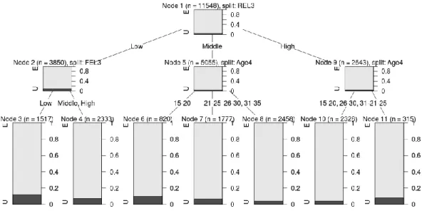
1.2.12 CHAID:
Chaid algorithm created by Kaas in 1980.It splits with Chi-Square test. Chaid built multiple tee unlike other algorithms. In addition Chaid built non-binary trees with is used simple algorithm. Chaid algorithm is appropriate for longer data analysis. Decision tree is built by basic algorithm Chaid as shown Figure 1.2.12.
Preparing predictors Merging categories
Selecting the split variable.
Chaid mathematical formula is below; F=WSS/(n−g)BSS/(g−1) ~ f(g-1).(n-g)
18
Figure 1.2.12:Decision Tree CHAID Algorithm
1.2.13 MARS:
Mars algorithm’s mean is Multivariate adaptive regression splines. Multiple regression function is used linear splines and their tensor products. MARS algorithm is presented by Jerome H. Friedmann in 1991.Mars has non-parametric regression technique. It is an extension of linear models non- iterative and interactions between variables. Mars is generated model with this formula:
F(x)= ∑ki=1ci. Bi(x)
The weighted sum of basis functions are defined Bi(x). It is a model. Each constant coefficient is ci. Every basis function Bi(x) uses three forms. They below:
A constant: It is just a term as a same time intercept.
A Hinge Function: This function contains form(0,x-const) or max(0, const-x). MARS selects variables and values automatically for nodes of hinge functions.
19
Two or more hinge functions are a product. These basis functions are interaction between two or more variables.
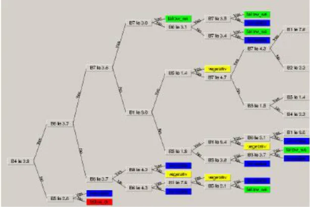
1.2.14 QUEST:
Quest algorithm can splits univariate and linear combination.
Each one input attribute and target attribute are relationship between for each split as shown 1.2.14. Also, they are calculated with the ANOVA F-test or Levene’s test (for ordinal and continuous attributes) Pearson’s chi-square (for nominal attributes).
Figure 1.2.14:Decision Tree Quest Algorithm
20
CART’s description is Classification and Regression Tree. Classification and Regression tree was built by breimann in 1984. They are continuation of chaid algorithm. CART features are
It has double refraction approach.
Cart algorithm can be classification and regression. It can use numeric and categorical inputs.
Cart is approve Gini Index. It can works missing value. It supports pruning ability.
CART has double refraction, so it preferred in high refraction computation. 1.2.15.1 Classification Trees:
Discrete target variable is used tree based modeling. Classification trees are used various measures of purity. Regression tree is not used various measures of purity. This is the most important difference from Regression Trees. Common measures of purity, Gini, entropy and Twoing.
Inititution: An ideal retention model can produce nodes. These nodes include defectors or non-defectors. They are only pure nodes.
1.2.15.2 Regression Trees:
Discrete target variable is used tree based modeling. Most intuitively appropriate method is useful for loss ratio analysis.
Greatest separation is given split. Its formula is: ∑ [y – E(y)] ²
21
It can be find nodes with minimal in variance. So it is biggest between variance. It’s like credibility theory. Every record is assigned the some that model. Every record in node. This model is step function.
More on Splitting Criteria: Gini purity of a node p(1-p)
where p = relative frequency of defectors
Entropy of a node –Σ p log p-[p * log(p) + (1- p) * log (1 – p) ] Max entropy/ Gini when p=5
Min entropy/ Gini when p=0 or 1
Gini might produce small but pure nodes
The “twoing” rule strikes a balance between purity and creating roughly equal-sized nodes.
How CART Selects the Optimal Tree:
It is used cross-validation for select optimal decision tree.
Built into the CART algorithm. Essential to the method; not an add-on Basic idea: “grow the tree” out as far as you can.Then “prune back”. CV: It is warning you on stop pruning time.
22
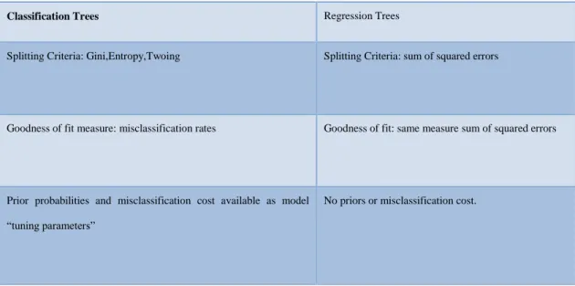
Classification Trees Regression Trees
Splitting Criteria: Gini,Entropy,Twoing Splitting Criteria: sum of squared errors
Goodness of fit measure: misclassification rates Goodness of fit: same measure sum of squared errors
Prior probabilities and misclassification cost available as model “tuning parameters”
No priors or misclassification cost.
Table 1.2.1.14:Classification Tree Vs. Regression Tree
1.2.15.3 Decision Tree Advantages and Disadvantages
Decision trees can easily understand and interpreted by end user. People can easily understand decision model after a little explanation.
It requires very quickly and simple pre-process data. Many becomes available data with minimal processing compared to alternative techniques.
It can adopt to add new scenario in tree.
You can determine worst, best and expected values for different scenarios with decision tree’s guide.
It uses a white box model. It is provided model when given a result. It can works with other decision tree techniques.
23
Many time optimum decision tree’s algorithm has NP-Complete complexity. So heuristic algorithm and greedy approach are used most of time.
Decision tree gives very complex calculations result when values are uncertain or many results are connected with others value.
1.3 Neural Network (NN) Based Approach
Neural Network is computers system. It emerged from the human brain’s learning ability, produce new information ability, predicting ability. Neural Network has 2 types. Biological Neural Network and Artificial Neural Network. We used Artificial Neural Network. Artificial Neural Network has 3 main layers.
1.3.1 Input Layer:
This layer where the inputs to neural network from outside world. It has neurons number of inputs.
1.3.2 Hidden Layer:
It has another name middle layer. This layer comes after the input layer. Hidden Layer’s neurons number independent other layers. This layer provides computation weight of inputs which are from input layer. Some neural networks do not have hidden layers. Too much neurons number extend the computation time and complicates to computation. But too much neurons useful for complex data.
24
This layer processing data from hidden layer and produce the output response of data from input layer. This layer send to output outside world. In feedback neural network output data calculate the new weight.
Neural networks are divided among themselves. Feedback neural network and feed forward neural network. I used feed forward neural network.
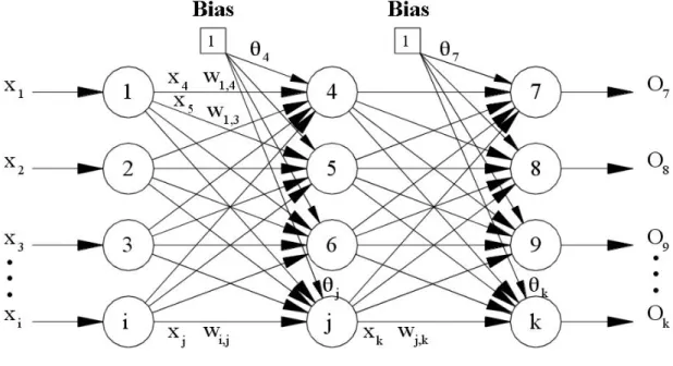
1.3.4 Feed Forward Neural Network:
It’s type of neural network. It is connect between the units but it doesnt form a directed cycle as shown Figure 1.3.4. It is different from recurrent neural.Data are respectively given input layer, hidden layer and output layer.
Figure 1.3.4:Artificial Neural Network Feed Forward
1.3.5 Feed Back Neural Network:
Feedback neural network distributed data previous layer or next layer. Feedback neural network is more dynamic than feed forward neural network as shown 1.3.5.
25
Figure:1.3.5 Artificial Neural Network Feed Back
1.3.6 Structure of Artificial Neural Cells:
Artificial neural cells’ structure is same as some of the biological neural cells. Artificial neurons comprise a neural network with establishing connection between neurons. Artificial neural cells have part, take input signs, collect of signs and give output same as biological neurons.
Artificial neural cells are;
Inputs Weights
Collection Function (Merge Function) Activation Function
26 Outputs
1.3.7 Inputs:
Inputs are the data from the neurons. Inputs can come from the outside, can come from another neural cells. This inputs send to nucleus neurons for merge data same as biological neural cells.
1.3.8 Weights:
Information which are come to artificial neural cells it is multiplied by the weight of their connection before reaching the neurons nucleus. Whereby the effect of inputs on the outputs to be produced can be adjusted. This weights value can be positive, negative or zero. Inputs no effect on outputs which has weight is zero.
1.3.9 Collection Function:
This function calculates total of results inputs multiplied by weights.
1.3.10 Activation Function:
This function takes the net inputs and determined the response had derived output. Generally activation function choice nonlinear function. Artificial neural neurons feature is nonlinear comes from activation functions is nonlinear function. Important point of choice activation function, can easy calculation of functions derivatives. In feedback network activation functions calculation is slowly. So function is should choice easy function. Nowadays used common activation function is “Sigmoid function” in N-Tier Sensor.
27 1.3.11 Cells Outputs:
Activation functions value is cells output value. This value can use output of artificial neural network or can use in network. Every cells has more inputs but has only one output. This output can connect any number cells.
28
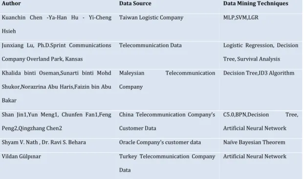
2. Related Works
Many different techniques are used churn analysis and prediction. Some data mining tools have these techniques. These techniques are used in academic researches or professional works. I studied on the techniques. Churn prediction model created to show between the differences. So, current studies are described as follows:
.
Author Data Source Data Mining Techniques
Kuanchin Chen -Ya-Han Hu - Yi-Cheng Hsieh
Taiwan Logistic Company MLP,SVM,LGR
Junxiang Lu, Ph.D.Sprint Communications Company Overland Park, Kansas
Telecommunication Data Logistic Regression, Decision Tree, Survival Analysis Khalida binti Oseman,Sunarti binti Mohd
Shukor,Norazrina Abu Haris,Faizin bin Abu Bakar
Maleysian Telecommunication Company
Decision Tree,ID3 Algorithm
Shan Jin1,Yun Meng1, Chunfen Fan1,Feng Peng2,Qingzhang Chen2
China Telecommunication Company’s Customer Data
C5.0,BPN,Decision Tree, Artificial Neural Network Shyam V. Nath , Dr. Ravi S. Behara Oracle Company’s customer data Naïve Bayesian Theorem Vildan Gülpınar Turkey Telecommunication Company
Data
Artificial Neural Network
Table 2:Related Works
Kuanchin Chen -Ya-Han Hu - Yi-Cheng Hsieh (2008) applied support vector machines (SVM),Logistic regression (LGR), Multilayer perceptron (MLP) in a Taiwan logistic company’s Churn context must be to create a churn model. Because, the customer churn prediction performance is determined and in the churn model is used to benchmarked to logistic regression and random estimate.
29
Junxiang Lu, Ph.D.Sprint Communications Company Overland Park, Kansas (2006) built a prediction model for Telecommunication company data by using survival analysis benchmarked to Decision tree and logistic regression. [3].
Khalida binti Oseman,Sunarti binti Mohd Shukor,Norazrina Abu Haris,Faizin bin Abu Bakar built prediction model for Maleysian Telecommunication company by using Decision Tree whic is ID3 algorithm.
Shan Jin,Yun Meng, Chunfen Fan,Feng Peng,Qingzhang Chen applied Neural Network and BPN algorithm, Decision Tree and C5.0 algorithm in China Telecommunication Company’s customer data. The customer churn prediction preformance of the Artificial Neural Network is benchmarked to Decision Tree C5.0. Shyam V. Nath , Dr. Ravi S. Behara applied Naive Bayesian Theorem for Churn analysis and Churn Customer prediction in Oracle Company’s Customer data.
Vildan Gürpınar is used Artificial Neural Network for churn prediction in Turkish Telecommunication data.
30
3 Material Methods
3.1 Customer Churn Data of UPS Turkey
This article used different types of variables which is UPS Turkey data. We have irregular data and they record different warehouses. We combined different data in single data warehouse. Our data types are customer marketing data , customer payment data , customer shipment data , customer personnel data and some specific data which are customer lost and damage records, customer complaint record. The dataset contains 20 variables worth of information of 11.46 customers. We use R programing language.
Data elimination with R programing: The variables are follows;
● Customer Code: It is represented by customer code which is created by logistics company.
● Customer Title: It is represented by customer commerce title.
● Status : Customer work status. It is prepared by marketing personnel.
● Previous Period Shipment Number: It is represented number of shipment in last year.
● This Period Shipment Number: It is represented number of shipment in this year.
● Previous Period Freight Cost : It represents the paid amount of shipment in last year.
● This Period Freight Cost: It represents the paid amount of shipment in this year.
31
● Main Sector : It represents customer’s job sector.
● Adv2012: It gives customer Average Daily of Volume in 2012. ● Adv2013 : It gives customer Average Daily of Volume in 2013. ● Adn2012 : It gives customer Average Daily of Net Revenue in 2012. ● Adn2013: It gives customer Average Daily of Net Revenue in 2013.
● DifVol : It represents the difference of Volume between this year and last year.
● RPP 2012: It represents the rate of Freight cost and Shipment number in 2012.
● RPP 2013: It represents the rate of Freight cost and Shipment number in 2013.
32
Adv2012 Adn2012 Adv2013 Adn2013 DifVol
RPP2012 RPP2013 ChurnStatus
3.843
27.500
6.447
45.021
2.604
7
7 No
1.191
7.497
2.886
18.761
1.695
6
7 No
276
2.181
1.504
6.126
1.228
8
4 No
2.185
13.018
3.047
18.018
862
6
6 No
465
2.069
1.257
5.860
792
4
5 No
230
1.849
981
6.867
752
8
7 No
1.827
10.947
2.493
15.619
666
6
6 No
2
19
0
0
-2
8
Yes
2
20
0
0
-2
9
Yes
2
8
0
0
-2
4
Yes
2
9
0
0
-2
4
Yes
2
16
1
9
-1
7
8 Yes
2
23
1
12
-1
10
10 Yes
Table3:Sample Data33 Fi gu re 2.2 :A rtif ic ial N eu ral N etw or k C h u rn M od el G rap h ic
34
Adv2012 Adv2013 Adn2012 Adn2013 DifVol RPP2012 RPP2013
Min. Value: 0TL 0TL 0TL 0TL 0 0.0 0 1st Quarter: 0TL 0TL 5.000 6TL 0 5 6 Median: 6TL 5TL 7TL 7TL 0 7 7 Mean: 50TL 47TL 8.75TL 25TL 0.5 8.75 9.25 3rd Quarter: 33TL 30TL 10 12TL 2 10 10 Max. Value: 996TL 997TL 313TL 999TL 862 305 401
35 Fi gu re 2.2 :D ec is ion T re e C h u rn M od el
36
Table 2.4:Decision Tree Prediction Rate
3.2. Generated Decision Tree Model and Prediction with R programing I generated model with R programing language. R is script language and statistical language. It has many data mining method and formula. I used R tree library. I have data in excel file. Firstly converted .csv format. Because .csv format is easily for reading data in R. After read data. After attach dataset I show summary for reviewed. Summary function give dataset min. value,1st quarter, mean, median , 3rd quarter and max. value. And attach dataset for processing. Codes and summary below; dataset<read.csv("/Users/newuser/Desktop/datamining/churn_companies.csv", head=TRUE,sep=";")
attach(dataset) summary(dataset)
After summary I prepared data for model generation. Firstly I created data frame and set modeling data in data frame. Next step I defined new column. And set this column churn status. In dataset Churn status represented “Durum” column. But in this data churn data represented 2 different keyword. Decliner and Lost represented churn customer. No change, gainer and conversion represented no churn customer. I set new column with condition. If customer is churn than column set with “yes” else “no”.
Churn<- data.frame(dataset , newcolumn) train<-sample(1:nrow(Churn),nrow(Churn)/2) test<- - train ,training_data<-Churn[train,]
37 df <- subset(training_data, select = -c(MusteriKodu,Unvani,Durum,OncekiDonemPaketAdedi,OncekiDonemNavlun ,DonemPaketAdedi,DonemNavlun,PazarlamaBolgesi,AnaSektor,NavlunDegisi mOrani,PaketDegisimOrani,PaketDegisimKodu) ) testing<-data<-Churn[test,] library(tree) mytree<-tree(newcolumn ~DifVol+Adn2012+Adn2013+RPP2013+Adv2012+Adv2013+RPP2012,data=Ch urn,method="class") plot(mytree) dim(mytree) summary(mytree)
38
If our model has acceptable rate of accuracy than we can use features in prediction. Predictions mathematical theorem is Entropy. Entropy is calculation of probability an event. In addition Entropy provide find randomness, uncertainty and unexpected situation. Entropy’s formula below;
E(CA)= p(a ,j)x − p(c a ,j)log p(c a ,j) Parameters:
E (C\Ak) = Ak area’s classification features Entropy j=1 P (ak, j)= probability of AK areas value same of j value.
P (ci \ ak, j) = probability of when ak value equals to j , classification value is ci. M = Number of value which are a area’s contain; j=1,kk,2,…,Mk N = Number of different class i = 1, 2,..., N, K = Number of areas;
k = 1,2,..., K.
Predict function in R include entropy. I used predict function in R programing language. First step I set testing dataset’s value in a table. I applied to predict function in testing dataset. I calculated average number of not equal to predicttion data. So that I found the correct prediction. And finally calculated summary of prediction and Show graphic.
Next step split data 2 data frame. First frame include training data. Training data contain %70 records in all of data. And second frame is testing date. It used for prediction. Second frame has %30 all of data. Last step is for model generation I added tree library and used tree function. It has formula for model generation. First parameter is Condition column name, and second parameter is which features are used for modeling and affected for churn status. And last parameter I set the tree
39
method. I choose class method. It is represented classification method. When generated model I showed it in graphic. R programing language has good graphic. And showed summary of model. Codes and model graphic are below;
tree_pred<-predict(mytree,df,type="class") table(tree_pred,Churn$newcolumn) mean(tree_pred!=) summary(tree_pred) plot(tree_pred) print(tree_pred) error_rate<-(1117+315)/(5137+5030)*100 print(error_rate) summary(mytree)
3.3 Generated Neural Network Model and Prediction with R programing
I used Artificial Neural network in R programing. It’s called neuralnet in R. First step I prepared data for model generation. I split data for training data set. I split between 1 to 8000 rows. And I split 8001 to 11599 rows for testing dataset. After split data I used 3 library. Neuralnet, MASS , grid. I attached them in my script. Neuralnet library accepted only matrix format data. So I converted my data frame to matrix. Next step I used neuralnet formula. First parameter is same of tree library.
40
Second parameter I taken features about possibility affected on model. Neural network has specific parameters in R programing. I studied on them.
Hidden:
It is represented number of neurons in hidden layer. I choose hidden 2. Because If hidden number is big than computation is slowly. It is enough my computation.
Threshold:
It is threshold value for stop the error function. In addition threshold is represented outlier data. Threshold has default value is 0.001. I set threshold 0.1.Because my data are regular and relation.
Life Sign:
It is represented by length of string. String is shows information about model. I choose minimal value. Whatever it can be maximum or none.
Linear Output:
It is represented by computation logic description. I didn’t need it. So I set this parameter FALSE.
41 Codes are below;
dataset<-read.csv("/Users/newuser/Desktop/datamining/churn_companies.csv",head=TR UE,sep=";") attach(dataset) trainset<-dataset[1:8000,] testset<-dataset[8001:11846,] library(neuralnet) library(MASS) library(grid)
m <- model.matrix( ~ ChurnStatusNumeric + RPP2012 +RPP2013+DifVol+ Adv2013 + Adn2013+ Adv2012 + Adn2012, data =trainset )
n <- model.matrix( ~ ChurnStatusNumeric + RPP2012 +RPP2013+DifVol+ Adv2013 + Adn2013+ Adv2012 + Adn2012, data =testset )
churnmodel<- neuralnet(ChurnStatusNumeric ~ RPP2012 +RPP2013+DifVol+ Adv2013 + Adn2013+ Adv2012 + Adn2012, m, hidden = 2, lifesign = "minimal",linear.output = FALSE, threshold = 0.1)
42
Prediction function is used in R after model generation. I calculated prediction and calculate summary. Summary gave me prediction status. 1 number is represented prediction, 0 number is represented don predictive. Summary mean is 0.9526761. It showed me %96 correct prediction.
Codes are below;
temp_test <- subset(testset, select =
c("RPP2012","RPP2013","DifVol","Adn2013","Adv2013","Adv2012","Adn2 012"))
churnmodel.results <- compute(churnmodel, temp_test)
summary(churnmodel.results)
results <- data.frame(actual = testset$ChurnStatus, prediction = churnmodel.results$net.result)
results[1:20, ]
results$prediction <- round(results$prediction)
43
4. Result And Discussion
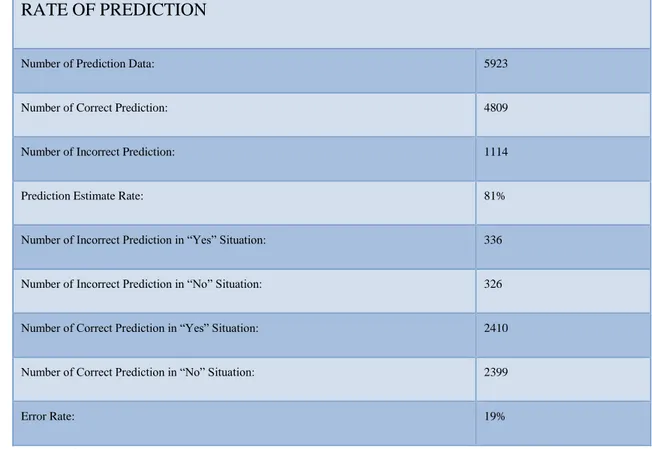
4.1 Decision True Churn Prediction Results
Decision Tree churn prediction is given 81% correct prediction rate.
RATE OF PREDICTION
Number of Prediction Data: 5923
Number of Correct Prediction: 4809
Number of Incorrect Prediction: 1114
Prediction Estimate Rate: 81%
Number of Incorrect Prediction in “Yes” Situation: 336
Number of Incorrect Prediction in “No” Situation: 326
Number of Correct Prediction in “Yes” Situation: 2410
Number of Correct Prediction in “No” Situation: 2399
Error Rate: 19%
44
4.2 Artificial Neural Network Churn Prediction Results Artificial Neural Network Prediction
Decision Tree churn prediction is given 97% correct prediction rate.
RATE OF PREDICTION
Number of Prediction Data: 3846
Number of Correct Prediction: 3730
Number of Incorrect Prediction: 116
Prediction Estimate Rate: 97%
Error Rate: 3%
45
4.3 Compare Decision Tree and Artificial Neural Network Churn Analysis: CART algorithm is used to create decision tree model. ”Yes” keyword is represented “churn customer” in model. The first node is affected by Difference Volume feature. If Difference Volume less than -05, customer churn status is “yes”. This model is used to estimate churn status. 4.809 item is predicted correctly.1114 item is predicted incorrectly. Correct prediction rate is % 81.
At the same time Artificial Neural Network is also used to make the same prediction. Neural network shows relative features with weighted. Both of the method shows that most important feature is Difference Volume. Difference Volume weight is 250.81071. Prediction with Neural Network resulted %96 accuracy. Therefore neural network’s prediction is better than decision tree.
Decision tree can easily be understood by end-user. But main reason is find the probability of customer churn. So neural network analysis is better for company for churn prediction. The neural network also presents the most important feature.
46
CONCLUSION
Nowadays customer churn analysis and retention of valuable customers are more important in logistics market challenge. In the past, especially telecommunication companies used churn analysis, but today churn analysis is very important for all of sectors. In this article, important point is the application of using data mining techniques in churn analysis. In this study, we observed Artificial neural network better than decision tree for churn analysis and prediction churn customer at the same time. Decision tree is a very basic data mining method, but the most popular technique is neural network, and it can predicted by churn customer more correctly than the decision tree. Thereby, companies can achieve true decision making with artificial neural network churn analysis.
47
REFERENCES
[1]Kuanchin Chen -Ya-Han Hu-Yi-Cheng Hsieh(2014).Predicting customer churn from valuable B2Bcustomers in the logistics industry: a case study
[2]Junxiang Lu, Ph.D.Sprint Communications Company Overland Park, Kansas(2001).Predicting Customer Churn in the Telecommunications Industry –– An Application of Survival Analysis Modeling Using SAS.
[3]Khalida binti Oseman,Sunarti binti Mohd Shukor,Norazrina Abu Haris,Faizin bin Abu Bakar(2010).Data Mining in Churn Analysis Model for Telecommunication Industry.
[4]Shan Jin1,Yun Meng1, Chunfen Fan1,Feng Peng2,Qingzhang Chen(2005).The Research on Applying Data Mining to Telecom Churn Management.
[5]Shyam V. Nath , Dr. Ravi S. Behara (2014).Customer Churn Analysis in the Wireless Industry: A Data Mining Approach.
[6]Vildan Gülpınar(2013).Customer Churn Analysis in the Turkish Telecomunication Market With The Help Of The Artificial Neural Networks And Social Network Analyses.
[7]Ali Rodan,1 Ayham Fayyoumi,2 Hossam Faris,1 Jamal Alsakran,1 and Omar Al-Kadi1(2015).Negative Correlation Learning for Customer Churn Prediction: A Comparison Study.
[8]Omar Adwan, Hossam Faris, Khalid Jaradat, Osama Harfoushi, Nazeeh Ghatasheh(2014).Predicting Customer Churn in Telecom Industry using Multilayer Preceptron Neural Networks: Modeling and Analysis.
48
[9]Anuj Sharma-Dr. Prabin Kumar Panigrahi(2011). A Neural Network based Approach for Predicting Customer Churn in Cellular Network Services.