Electromagnetic engineering in the 21st century: challenges and perspectives

Electromagnetic Engineering in the 21

st

Century:

Challenges and Perspectives

Leopold B. FELSEN

Dept. of Aerospace & Mechanical Engineering and Dept. of Electrical & Computer Engineering, Boston University, 110 Cummington Street, MA 02215, USA (part time) Also University Professor Emeritus, Polytechnic University, Brooklyn, NY 11201, USA

e-mail: lfelsen@bu.edu

Levent SEVG˙I

Electronics and Communication Engineering Dept., Do˘gu¸s University, Zeamet Sok. No. 21, Acıbadem, ˙Istanbul-TURKEY

e-mail: lsevgi@dogus.edu.tr

Abstract

This paper aims at a broad-brush look at certain technological and educational challenges that con-front wave-oriented electromagnetic (EM) engineering in the 21st century, in a complex computer and technology-driven world with rapidly shifting societal and technical priorities. Simulation strategies for complex EM systems, both analytic and numerical, are reviewed and categorized, and are illustrated on selected practical complex multicomponent system scenarios currently under investigation in Turkey. Educational issues to ensure proper multidisciplinary exposure of new generations of computer-weaned students, who will have to deal with these problems, are touched upon as well.

Key Words:electromagnetic engineering, electromagnetic education, analytical model, numerical model, numerical simulation, engineering challenges, fields and networks, verification, validation, accreditation, calibration

1.

Introduction

1.1.

Technical challenges

Many applications in science and technology rely increasingly on electromagnetic field computations in either man-made or natural complex structures. Wireless communication systems, for example, pose challenging problems with respect to field propagation prediction, microwave hardware design, compatibility issues, biological hazards, etc. Since different problems have their own combination of geometrical features and scales, frequency ranges, dielectric inhomogeneities, etc., no single method is best suited for handling all possible cases; instead, a combination of methods (hybridization) is needed to attain the greatest flexibility and efficiency. Relations between field theory and network theory [1-4] play an important role in this respect. The necessity for hybrid methods has already been recognized in the past [5,6]: for example, in scattering and antenna problems (see, e.g. References [7-15]), techniques have been devised that combine the Method of Moments (MoM) and the geometrical theory of diffraction (GTD) or physical optics (PO) [16,17]. Similarly, numerical methods such as finite elements (FEM) or finite differences have been considered

in conjunction with MOM [18,19], with integral equations [20,21], with boundary integrals [22], with modal techniques [23], with multipole methods [24], etc. Combinations of other methods, e.g. boundary-contour and mode-matching [25] or hybrid electric field integral equations (EFIE) and magnetic field integral equations (MFIE) denoted as HEM [26], have also been proposed. This list of contributions, though necessarily incomplete, indicates that this topic is of considerable interest. The methods enumerated above have typically been applied to solve a specific class of problems efficiently by matching the method to the perceived phenomenology, as in References [10-12]. Despite these apparent diversities there are certain features common to all hybrid methods; namely, that the overall problem gets partitioned self-consistently, in a problem-matched manner, into interacting subdomain (SD) problems. An architecture, i.e. a structure that addresses complexity systematically and with reasonable generality, can be helpful here. An architecture does not solve a problem but it can provide a systematic framework for posing proper questions.

Complexity, in the context of waves, encompasses many scales which are conveniently referenced to the related wavelengths λ =2 π c/ ω in the interrogating wave signal, where c is the wave speed in a reference ambient medium and ω is the radian frequency. These relative scales si/ λ can be associated with

physical dimensions si≡di; wavelengths si ≡ λi in various materials; temporal widths si≡Tiof the signal

spectra; sampling window widths si ≡Wi in the processing of data, etc. Of special interest are complex

environments with at least some constituent physical dimensions di/λi>> 1 . Under these short wavelength

(high frequency) conditions, wavefields can often be organized around propagating (progressing) ray-like or oscillatory (standing) mode-like wave objects (observables) which are tied to complementary physical wave phenomenologies and, when matched to the problem, can give rise to efficient numerical algorithms for the computation of the complex wavefield. Purely numerical techniques under these conditions are inefficient because the required discretization at scales ∆i, which are fractions of the wavelength λi,renders the problem

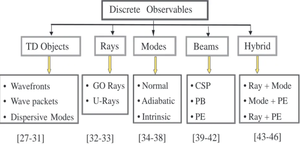
numerically large. Some examples of useful waveobjects in the frequency and time domains are shown in Figure 1.The wave modeler must decide how to parameterize a complex physical problem so as to take best advantage of the wave-based and computational tools at his/her disposal. The above technical challenges are dealt with in Section 2.

Discrete Observables

• GO Rays

• U-Rays

Rays

Modes

Beams

Hybrid

• Normal

• Adiabatic

• Intrinsic

• CSP

• PB

• PE

• Ray + Mode

• Mode + PE

• Ray + PE

• Wavefronts

• Wave packets

• Dispersive Modes

TD Objects

[27-31]

[32-33]

[34-38]

[39-42]

[43-46]

Figure 1. Discrete wave observables in EM (TD: Time-domain, GO: Geometric Optics, U: Uniformized, CSP:

1.2.

Educational challenges

Having described the technical challenges (see Section 1.1), it is necessary to educate new student populations in the skills required to deal with them. Some approaches by different functionaries in the educational establishment to meeting these challenges are summarized in Section 3.

2.

Technical Challenges: Complexity

2.1.

Fields, networks and architecture

A general framework for decomposing an overall complex problem space into interacting subdomains (SD) and subsequent treatment of the problem via field and network theories is pictured in Figure 2. With reference to Figure 2, we assume that the problem geometry is specified, as are the sources and field observables, the latter being defined as the fields that can be measured on specified reference surfaces.

R1 R2 R3 R0 B₁₂ B13 B23 B21 B31 B₃₂ B02 B20 B10 B₀₁ B03 B30

Partitioning the Problem Space Ri: Subdomain, i=1,2 ..

Bij: Interface between subdomains Ri and Rj

Connection Relations (for fields) Complex domain Segmentation Subdomain equations (matrix form) Network topology Subdomain Relations (for fields) Network Solution Field equation in Tableau form Discretization Options: Topological alternatives Numerical alternatives Accesible and internal observables:

Primary and secondary field variables

Alternative Green’s functions

Choice of field basis functions

Figure 2. (a) Complexity partitioning into SDs, (b) Schematic view of the proposed methodology [2-4]. The flowchart on the left highlights the main steps for the generalized network formulation of the field problem; the available options are summarized on the right.

After partitioning of the overall complex problem domain into SDs which are selected so as to facilitate numerical or analytical treatment, we need to specify primary and secondary field variables. For each SD, the secondary field variables are defined as the response to the impressed primary field variables. The choice

of primary and secondary fields affects the type of boundary conditions pertaining to a particular subdomain and, therefore, the corresponding alternative Green’s function representation. In fact, in order to separate one subdomain from adjacent regions, we apply the equivalance theorem [47, pp. 38-46]; for example if, on one aperture, electric fields are selected as primary fields, then the magnetic field is the secondary field, yielding an admittance description with the aperture replaced by a perfect electrical conductor (PEC). For each particular selection of primary and secondary fields, the corresponding convergence properties, wave patterns and wave phenomenology determine the problem strategy.

Next we distinguish between subdomain relations and connection relations. For each SD and corre-sponding boundary conditions, the secondary fields express how that particular SD reacts under the excita-tion provided by the primary field. Each SD with its subdomain relaexcita-tions is therefore distincted from other SDs. Connection networks implement the topological relations for fields, i.e. the continuity of the tangential field components at common interfaces between adjacent SDs. Models of partitioning for electromagnetic field computation correspond to network models used in circuit theory as follows:

• Relations at boundaries between adjacent subdomains ↔ topological relations in a network;

• Subdomain relations per se ↔ laws governing the behavior of circuit elements such as resistors, inductors, capacitors, etc.

Network formulations of field problems have been employed extensively after World War II in the design of microwave, optical and other closed and open waveguiding and radiating systems [1]. With the current evolution of exotic materials for bulk wave control, guided wave applications, radiators, etc., it can be anticipated that network representations of field problems will again receive attention and that novel SD circuit elements connected via novel transmission lines (propagators) will appear in complex guiding, radiating and resonating architectures. The wave modeler’s role is to provide, whenever possible, the appropriate wave-physical footprints of what transpires inside the SD “black boxes”, thereby incorporating wave-based preconditioning in systems algorithms.

2.2.

Numerical simulations

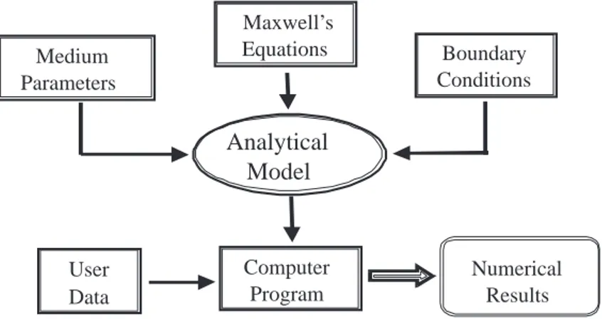
Analytical models based on either field theory or network theory express solutions for the independent variables, such as electric and magnetic field components or input-output voltages and currents, in terms of analytic functions (such as SINE or COSINE functions, Bessel and/or Hankel Series, etc.). A computer program is required only to calculate an output value for a given input supplied by the user (see flow-chart in Figure 3).

Alternatively, for each SD, there is also the option to select a specific problem-matched purely numerical method. For example, we may divide the overall structure in such a way that it is convenient to use an integral equation approach in one SD, a finite element solution in another SD and a boundary element method in a third SD. Closely related to the above choice is the selection of expansion and testing basis function sets at the boundary of each subdomain which pertains to the discretization of the field equations. Here the options are: use of entire domain or subdomain basis functions; eigenfunction (modal) expansions; edge-corrected basis functions, etc.

Maxwell’s Equations

Analytical

Model

Figure 3. Analytic-model-based solution flow chart

Numerical models can be viewed differently from the developer’s and the user’s perspectives [48]. De-velopers deal primarily with the conceptual suitability and implementational steps of the codes (verification), while the users are more involved in computation and application. Both are concerned with validation, al-though users are often tempted to apply codes in a manner never envisioned by the developers, thus making validation an especially sensitive topic. From the developer’s perspective, the process of developing a numer-ical model involves conceptualization, formulation, numernumer-ical implementation, computation and validation. On the other hand, the user’s perspective involves the problem, i.e., choosing a problem-matched approach and the application steps. A developer needs to know how the code works but the user needs to know what it can do.

Characterization and comparison of numerical simulators basically relies on accuracy and reliability, efficiency and, finally, applicability. Someone who deals with numerical simulation is in a quite similar position to that of an experimenter. They both need to understand requirements for their particular problem in terms of basic EM phenomena, but both also need to depend on complex tools that they did not design in order to accomplish their particular goals.

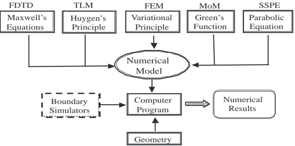
The flow-chart of a numerical model is given in Figure 4 [48]. The principal algorithm models the intrinsic behavior of EM fields without reference to specific boundary and material configurations. Some well-known and widely used numerical approaches are listed in the figure. As shown, the generic numerical model is applied from the very beginning and is augmented by boundary simulators and/or other peripheral units, such as near-field far-field transformations. Different problems (with respect to geometry and medium parameters) can be accommodated by such models. More specifically, in the FDTD (finite-difference time-domain) technique [49], the physical geometry is divided into small rectangular (mostly cubical) cells. Thus, via FDTD, Maxwell’s equations are discretized directly in the time domain. On the other hand, the TLM (transmission line matrix) method [50] uses Huygen’s principle, i.e., it is based on circuit theory, and the discretization of fields (the continuous system) is effected by an array of three-dimensional (3D) lumped elements. Thus, the TLM technique involves two basic steps: (i) replacing the field problem by the equivalent network and establishing the connection between the field and network quantities; (ii) solving the equivalent network by iterative methods.

FEM (finite element model) analysis [51] of a problem includes (i) discretization of the solution region into a finite number of sub-regions or elements, (ii) derivation of the governing equations for a typical element, (iii) assembling all elements in the solution region, and (iv) solving the system of equations obtained. The step that makes FEM different from other methods is the need to derive the governing equations for the elements,

thereby implying that analytical representations should be obtained for the elements before proceeding to the general solution. This is similar to the requirement to derive a Green’s function in the MoM (Method of Moments) technique. One major difficulty encountered in FEM analysis is data preparation, which is essentially element generation; therefore special mesh generators have been developed for this purpose.

Parabolic Equation SSPE Maxwell’s Equations Numerical Model Variational Principle Huygen’s Principle Computer Program Numerical Results Boundary Simulators FDTD TLM FEM Green’s Function MoM Geometry

Figure 4. Numerical-model-based solution flow chart

MoM [52] is based on solving (via discretization) complex integral equations by reducing them to a system of linear equations. The equation solved by MoM generally has the form of an electric field integral equation (EFIE) or a magnetic field integral equation (MFIE). Although MoM can be applied also in the time domain, the majority of these equations are set in the frequency domain. Recently, the Fast Multipole Method (FMM), based on MoM, and the Multilevel Fast Multipole Algorithm have been introduced [53], which reduce the number of unknowns in matrix form solutions of integral representations for the fields.

The SSPE (split-step parabolic equation) technique, widely used in propagation scenarios, implements the solution of the one-way parabolic type wave equation (see [54] and references therein). It neglects back-scatter effects and is valid in regions close to near-axial propagation. It is an initial value problem, mostly used in 2D, where transverse and/or longitudinal characteristics can be included. An initial transverse field distribution is injected, and propagated longitudinally through a medium defined by its refractive index profile so as to yield the transverse field profile at the next range step. By sequential operations accessing the transverse spatial and wavenumber domains via the fast Fourier transform (FFT) and inverse FFT, respectively, one may obtain the transverse field profile at any range. SSPE cannot directly handle general boundary conditions at the surface, and must be complemented by special techniques.

Whether analytical or numerical, models need to be coded for calculations by computer. While the model in analytical solutions is constructed according to the geometry of the problem (i.e., boundary conditions and medium parameters), the numerical model is general and the geometry of the problem (together with the input parameters) is supplied after the model is built. That is, the boundary and/or initial conditions are supplied externally to the numerical model together with the medium parameters, operating frequency, signal bandwidth, etc. Once these are specified, simulations are run and sets of observable-based output parameters are computed for the given set of input parameters. The algorithms in Figure 4 are all model proof; i.e., there is no need to test the validity of Maxwell’s equations for FDTD, or of circuit theory for TLM. However, one must establish whether the model is built “correctly” and under what conditions it is valid. This leads to testing for stability (since the solution is iterative) and for numerical dispersion (since the wave physics is traced in the discrete environment).

For very complex multi-function systems the verification strategy is generally not apparent a priori. A typical scenario might involve two microwave radars and one HF (high frequency) radar to cover a coastal region bounding an ocean with surface and air-borne targets. How should the simulator be built and what will the requirements be for model verification? There is no single procedure for constructing this simulator; it essentially depends on the problem requirements. For example, one may need to simulate a target signal as a detailed time sequence that accounts for target fluctuations, noise, clutter and interference. This requires stochastic modeling of each target and its environment. If a target tracker is to be simulated, a target can only be represented as a single “detected” or “missed” decision. Therefore, verification, validation and accreditation (VV&A) has become one of the major concerns in numerical simulation procedures, and they are problem-dependent.

2.3.

Verification, validation, accreditation (VV&A) and calibration of

simula-tion algorithms

Simulation in engineering usually refers to the process of representing the dynamical behavior of a “real” system in terms of the behavior of an idealized more manageable model system implemented through computation via a simulator. The simulator comprises a program or a series of programs developed to implement and execute simulations with well-defined relations between model objects. These relations are, by definition, mathematical relations.

“Real - world” Problem Entity Computer Model Conceptual Model OPERATIONAL VALIDITY CONCEPTUAL & MODEL VALIDITY SOFTWARE Computer Programming & Implementation DATA VALIDITY VERIFICATION

Experimentation Analysis& Modelling

Figure 5. Simulation concepts, verification, validation and accreditation [55]

The fundamental building blocks of a simulation are [55] the real-world problem entity being simulated, a conceptual model representation of that entity, and the computer model implementation of the conceptual model (see Figure 5). The suitability of the conceptual model, verification of the software and data validity are the technical processes that must be addressed to make a model credible. Credibility resides on two important checks that must be made in every simulation: validation and verification. As summarized in

[56], validation is the process of determining that the right model is built, whereas verification is designed to see if the model is built right.

Verification involves debugging and ensuring consistency between the computer code and the model. Validation involves comparing the model’s output with the behavior of the real problem, and focuses on three questions [55]:

1. Conceptual Validity: Does the model adequately represent the real-world system?

2. Operational Validity: Are the model-generated behavioral data consistent with characteristics of the actual system?

3. Believability: Does the user have confidence in the model’s results?

Credibility (or accreditation) of the simulation depends also on the characteristics of the real-world system (the problem). Three versions of the real world have to be distinguished [55]:

• The system exists and its outputs can be compared with the simulated results • The system exists but is not available for direct experimentation (e.g. a plane crash)

• The system is yet to be designed; validation here is in the sense of convincing ourselves and others that observed model behavior represents the proposed reference system if it is implemented

Calibration is the process of parameter estimation for a model. It is concerned with tuning of existing parameters and usually does not involve the introduction of new ones, which would change the model structure. Calibration is also referred to as parameter optimization involved in system identification or during experimental design.

3.

Challenging Simulation Examples

As discussed in Section 2, simulation is required or preferred when (i) it is too expensive and/or dangereous to perform real tests and/or experiments on an existing multifunction complex system; (ii) the system is not available or cannot be prepared for a real scenario. This Section contains brief illustrations of certain challenging EM numerical simulation problems currently under investigation in Turkey.

3.1.

Integrated surveillance and control systems

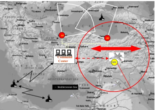
Electronic surveillance systems have been widely used for both military and commercial purposes, from intrusion alarms to integrated defense systems. In addition to surveillance it may also be required to have communication, control, command and fire-control in some of the surveillance systems. The simulation of these systems requires understanding of the sensor physics in the preparation of intelligent detection and tracking algorithms.

A typical integrated surveillance system is pictured in Figure 6, whose function is continuous moni-toring of surface activity on the Black Sea (using two surface wave HF radars) and air activity in Eastern Turkey (using an onboard microwave radar) as an example [57-60]. Assuming that reliable sensor simulators are available; certain aspects still need to be addressed in the design of an integrated system:

• HF radar location for optimum coverage • site specifications

• aircraft altitude for optimum air coverage • aircraft speed for minimum revisit time

• number of targets that can be monitored continuously

• speed, capacity, etc. required for communication links, software and hardware • overall performance of the integrated system for different scenarios.

Simulation is the only tool for dealing with such complexity and for exploring alternatives as well as “what if ?” type scenarios.

Command Center

HF

HF

MW

Figure 6. A typical integrated, multi-purpose surveillance system for Turkey

A rugged mountain border line surveillance scenario between two non-friendly countries is pictured in Figure 7. Here, decisions via simulations must be made concerning the type of sensors (e.g., HF, VHF, microwave radars, optical, thermal cameras, etc.), their parameters and optimum location [61-64].

3.2.

Radar cross section (RCS) reduction

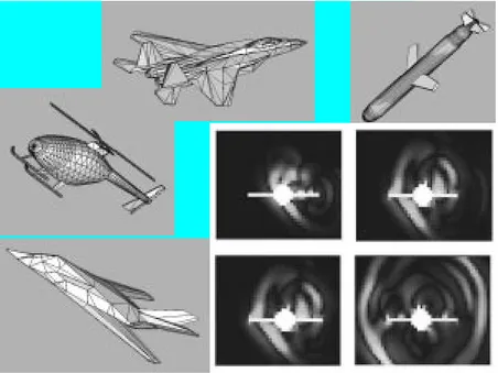
Another challenging area in numerical simulation is RCS prediction and “low visibility” target design. As shown in Figure 8, low RCS airborne targets may be designed by (i) altering the geometry, (ii) using radar absorbing materials (RAM), (iii) using active/passive cancellation techniques (e.g., via an array of active dipoles). RCS numerical modeling and target design can be effected through various techniques and/or their hybridized forms: FDTD, TLM, FEM and MOM (especially FMM), all of which can be applied to arbitrary target shapes. The RCS resonance region, where the dimension of the target is in the order of

the radar wavelength, is of special interest because that is where the structure of the target dominates the RCS behavior. For RCS analysis of air and surface targets with HF radars, see [65-67]. As the frequency increases, the requirement to model the target in detail exceeds the capacities of the purely numerical procedures mentioned above even with use of parallel processing, thereby necessitating hybridization. This can be done either by combining two numerical techniques, or by combining one numerical technique with one of the analytic high frequency, physics-based asymptotic forms, such as geometrical optics (GO), physical optics (PO), geometrical theory of Diffraction (GTD), physical theory of diffraction (PTD), uniform theory of diffraction (UTD), etc. RCS modeling for large bodies with small cracks, cavities or apertures, for example, is executed effectively by these hybrid techniques.

VHF? MW? IR? VHF? MF? IR?

Figure 7. Typical border-line multi-sensor surveillance system (MW: Microwave Radar, VHF: Very high frequency

radar, IR: Infrared Camera)

4.

Educational Challenges

Addressing the technical challenges posed by system complexity as in Section 2 requires a broad range of innovative, multi-disciplinary, physics-based, problem-matched analytical and computational skills that are not adequately covered in conventional engineering curricula. A great many higher educational institutions are now actively engaged in efforts to define “what makes a modern engineer”, and to design curricula for teaching the necessary skills to a computer-weaned generation of students, with access to the internet and consequent globalization of information.

Some of these issues were discussed by a panel of high-level specialists in educational matters during the Plenary Session entitled “Engineering Education in the 21st _{Century: Issues and Perspectives”, organized}

by L. B. Felsen at the International Conference on Electromagnetics in Advanced Applications (ICEAA) which was held in Torino, Italy, during September 10-14, 2001. A summary of the papers presented in this session is scheduled for publication in the December 2001 issue of IEEE Antennas and Propagation Magazine. In order to indicate the scope of the lectures and ensuing discussions, we list below the titles of the contributions:

Figure 8. Typical low RCS targets and simulations and near field FDTD simulations

1. “Teaching Analysis to a Computer-weaned Generation: Asking questions”, Prof. Leopold B. Felsen, Dept. of Aerospace and Mechanical Engineering, Boston University, USA

2. “Teaching Electromagnetics to a Knowledge-saturated Generation”, Prof. Weng C. Chew, Dept. of Electrical Engineering, University of Illinois, Urbana-Champaign, USA

3. “A Professional Master Degree on the Internet”, Danilo Erricolo, et al. College of Electrical Engineer-ing, University of Illinois, Chicago, USA

4. “Technology-based Education: Multimedia Assets and Interactive Models for Modern EM Education”, Prof. Magdy F. Iskander, Dept. of Electrical Engineering, University of Utah, USA

5. “Internationalism and Implications for Engineering Education: Changes in the European Educational System”, Giancarlo Spinelli, President, Center for International Relations, Politecnico, Milano, Italy

6. “Engineering education: Where Do We Go From Here?”, David C. Chang, President, Polytechnic University, Brooklyn, NY, USA

7. “Challenges to Engineering Education in the 21st _{Century”, Rodolfo Zich, President, Politechnico di}

Torino, Italy

5.

Conclusions

In this brief glimpse at certain issues which confront wave-oriented EM engineering in the 21st _century,

we have attempted to identify challenges, both technical and educational, that deserve the attention of the engineering community as a part of society in a rapidly changing, internet-driven globalized world of enermous intertwined social-technical complexity. The explosive growth of computer capabilities has revolutionized communication and the analysis of complex systems, and has made interdisciplinary exposure necessary in modern engineering.

The EM engineer, either individually or as member of a team, can play an important role in this technically diverse mosaic, as has been illustrated by analytic, numerical and hybrid options for propagation modeling in complex large environments, and by inclusion of selected example scenarios currently under investigation in Turkey. Rapid scientific advances, followed by rapid advances in technologies, are here to stay, and the engineering community must be prepared to adapt to frequent shifts in technical priorities.

Acknowledgement

L. B. Felsen acknowledges partial support from ODDR&E under MURI Grants ARO DAAG55-97-1-0013 and AFOSR F49620-96-1-0028, from the Engineering Research Centers Program of the National Science Foundation under award no EEC9986821, from the US-Israel Binational Science Foundation, Jerusalem, Israel, under Grant No. 9900448 and from the Polytechnic University.

References

[1] L. B. Felsen, N. Marcuvitz, Radiation and Scattering of Waves, Prentice-Hall, New Jersey, 1973.

[2] L. B. Felsen, M. Mongiardo, P. Russer, “Electromagnetic Field Representations and Computations in Complex Structures: I. Complexity Architecture and Generalized Network Forumulation”, Int. J. Numerical Modeling, Vol. 15(1), pp. 93-107, 2002.

[3] L. B. Felsen, M. Mongiardo, P. Russer, “Electromagnetic Field Representations and Computations in Complex Structures: II. Alternative Green’s Functions, Int. J. Numerical Modeling, Vol. 15(1), pp. 109-125, 2002. [4] P. Russer, M. Mongiardo, L. B. Felsen, “Electromagnetic Field Representations and Computations in

Com-plex Structures: III. Network Representations of the Connecting and Subdomain Circuits, Int. J. Numerical Modeling, Vol. 15(1), pp. 127-145, 2002.

[5] E. K. Miller, “A Selective Survey of Computational Electromagnetics”, IEEE Trans. Antennas and Propagat., Vol. 36, pp. 1288-1305, 1988.

[6] G. A. Thiele, “Overview of Selected Hybrid Methods in Radiating Systems Analysis”, Proceeding of IEEE, Vol. 80, pp. 66-78, 1992.

[7] L.N. Medgyesi-Mitschang, D. S. Wang, “Review of Hybrid Methods on Antenna Theory”, Annales of Telecom-munications, Vol. 44(9), 1989.

[8] W. D. Burnside, C. L. Yu, R. J. Marhefka, “A Technique to Combine Geometrical Theory of Diffraction and Moment Methods”, IEEE Trans. Antennas and Propagat., Vol. 23, pp. 551-558, 1975.

[9] G. A. Thiele, T. H. Newhouse, “A Hybrid Technique for Combining Moment Methods with the Geometrical Theory of Diffraction”, IEEE Trans. Antennas and Propagat., Vol. 23, pp. 551-558, 1975.

[10] T. J. Kim, G. A. Thiele, “A hybrid diffraction Technique - General Theory and Applications”, IEEE Trans. Antennas and Propagat., Vol. 30, pp. 551-888, 89730

[11] L.N. Medgyesi-Mitschang, D. S. Wang, “Hybrid Solution for Scattering from Perfectly Conducting Bodies of Revolution”, IEEE Trans. Antennas and Propagat., Vol. 31, pp. 570-583, 1983.

[12] L.N. Medgyesi-Mitschang, D. S. Wang, “Hybrid Solutions from Large Bodies of Revolution with Material Discontinuities and Coatings”, IEEE Trans. Antennas and Propagat., Vol. 32, pp. 717-723, 1984.

[13] L.N. Medgyesi-Mitschang, D. S. Wang, “Hybrid Solutions for Large Impedance Coated Bodies of Revolution”, IEEE Trans. Antennas and Propagat., Vol. 34, pp. 1319-1329, 1986.

[14] D. S. Wang, “Current-based Hybrid Analysis for :Surface Wave Effects on Large Scatterers”, IEEE Trans. Antennas and Propagat., Vol. 39, pp. 839-850, 1991.

[15] D. P. Bouche, F. A. Molinct, R. Mittra, “Asymptotic and Hybrid Techniques in Electromagnetic Scattering”, Proceedings of IEEE, Vol. 81, pp. 1658-1684, 1993.

[16] U. Jakobus, F. M. Landstorfer, “Improved PO-MM hybrid Formulation for Scattering from three-dimensional Perfectly Conducting Bodies of Arbitrary Shape”, IEEE Trans. Antennas and Propagat., Vol. 43, pp. 162-169, 1995.

[17] U. Jakobus, F. M. Landstorfer, “Improved PO-MM hybrid Formulation by Accounting for Effects Perfectly Conducting Wedges”, IEEE Trans. Antennas and Propagat., Vol. 43, pp. 1123-1129, 1995.

[18] X. Yuang, D. R. Lynch, J. W. Struhbehn, “Coupling of Finite Element and the Moment Methods for Electro-magnetic Scattering from Inhomogeneous Objects”, IEEE Trans. Antennas and Propagat., Vol. 38, pp. 386-393, 1990.

[19] D. J. Hoppe, L. W. Epp, J. F. Lee, “A Hybrid Symmetric FEM-MOM Formulation Applied to Scattering by Inhomogeneous Bodies of Revolution”, IEEE Trans. Antennas and Propagat., Vol. 42, pp. 798-805, 1994. [20] C. Z. T. Cwik, V. Jamnejat, “Modeling three-dimensional Scatterers using a coupled Finite Element Integral

Equation Formulation”, IEEE Trans. Antennas and Propagat., Vol. 44, pp. 453-459, 1996.

[21] C. Z. T. Cwik, V. Jamnejat, “Modeling radiation with an Efficient hybrid Finite Element Integral Equation Waveguide Mode-matching Technique”, IEEE Trans. Antennas and Propagat., Vol. 45, pp. 34-39, 1997. [22] K. Ise, M. Koshiba, “Numerical Analysis of H-plane Waveguide Junctions by Combination of Finite and

Boundary Elements”, IEEE Trans. On Microwave Theory and Techniques., Vol. 36, pp. 1343-1351, 1988. [23] M. Mongiardo, R. Sorrentino, “Efficent and Versatile Analysis of Microwave Structures by combined Mode

Matching and Finite difference Methods”, IEEE Microwave Guided Wave Letters., Vol. 3, pp. 241-243, 1993. [24] N. Lu, J. M. Jin, “Application of Fast Multipole Method to Finite element Boundary-integral Solution of

Scattering Problems”, IEEE Trans. Antennas and Propagat., Vol. 44, pp. 781-786, 1997.

[25] J. M. Reiter, F. Arndt, “Hybrid Boundary-contour mode-matching Analysis of Arbitrary Shaped Waveguide Structures with Symmetry of Revolution”, IEEE Microwaves and Guided Wave Letters., Vol. 6, pp. 369-371, 1996.

[26] R. E. Hodges, Y. Rahmat-Samii, “An Iterative current-based Hybrid Method for Complex Structures”, IEEE Trans. Antennas and Propagat., Vol. 45, pp. 265-276, 1997.

[27] E. Heyman, L. B. Felsen, “A Wave Front Interpretation of the Singularity Expansion Method”, IEEE Trans. Antennas and Propagat., Vol. 33, pp. 706-718, Jul 1985.

[28] L. B. Felsen, “Progressing and Oscillatory Waves for Source-excited Propagation and Diffraction”, IEEE Trans. Antennas and Propagat., Vol. 32, pp. 775-796, 1984.

[29] L. B. Felsen, F. Niu, “Spectral Analysis and Synthesis Options for Short Pulse Radiation from a Point Dipole in a Grounded Dielectric Layer”, IEEE Trans. Antennas and Propagat., Vol. 41, pp. 747-754, 1993.

[30] F. Niu, L. B. Felsen, “Time Domain Leaky Modes on Layered Media: Dispersion Characteristics and Synthesis of Pulsed Radiation”, IEEE Trans. Antennas and Propagat., Vol. 41, pp. 755-761, 1993.

[31] F. Niu, L. B. Felsen, “Asymptotic Analysis and Numerical Evaluation of Short Pulse Radiation from a Dipole in a Grounded Dielectric layer”, IEEE Trans. Antennas and Propagat., Vol. 41, pp. 762-769, 1993.

[32] L. G. James, Geometric Theory of Diffraction for Electromagnetic Waves, IEE Electromagnetic Wave Series -I, Peter Peregrinus, London, 1976.

[33] A. Ishimaru, Electromagnetic Wave Propagation, Radiation and Scattering, Prentice Hall, Englewood Cliffs, New Jersey, 1991.

[34] A. D. Pierce, “Extension of Method of Normal Modes to Sound Propagation in an Almost Stratified Media”, J. Acoust. Soc. Am., Vol. 37, pp. 19-27, 1965.

[35] A. D. Pierce, “Guided Mode Disappearance During Upslope Propagation in Variable Depth Shallow Water Overlying a Fluid Bottom”, J. Acoust. Soc. Am., Vol. 72, pp. 523-631, 1982.

[36] J. M. Arnold, L. B. Felsen, “Intrinsic Modes in a Wedge-shaped Ocean”, J. Acoust. Soc. Am., Vol. 76, pp. 850-860, 1984.

[37] L. B. Felsen, L. Sevgi, “Adiabatic and Intrinsic Modes for Wave Propagation in Guiding Environments with Longitudinal and Transverse Variations: Formulation and Canonical Test”, IEEE Transactions on Antennas and Propagat. Vol. 39 No. 8, pp. 1130-1136, Aug. 1991.

[38] L. B. Felsen, L. Sevgi, “Adiabatic and Intrinsic Modes for Wave Propagation in Guiding Environments with Longitudinal and Transverse Variations: Continuously Refracting Media”, IEEE Transactions on Antennas and Propagat. Vol. 39 No. 8, pp. 1137-1143, Aug. 1991.

[39] G. Deschamps, “Gaussian Beams as a Bundle of Complex Rays”, Electronics Letters, Vol. 7, pp. 684-685, 1971. [40] L. B. Felsen, “Complex Rays”, Philips Res. Repts, Vol. 30, pp. 187-195, 1975.

[41] L. B. Felsen, “Rays, Modes and Beams in Optical Fibre Waveguides”, J. Acoust. Soc. Am., Vol. 66(8), pp. 751-760, Aug. 1976.

[42] E. Heyman, L. B. Felsen, “Gaussian Beam and Pulsed Beam Dynamics: Complex Source and Spectral Formu-lations within and beyond Paraxial Asymptotics”, J. Opt. Soc. Am., Vol. 18, pp. 1588-1611, 2001.

[43] T. Ishihara, L. B. Felsen, “Hybrid (Ray)-(Parabolic Equation) Analysis of Propagation in Ocean Acoustic Guiding Environments”, J. Acoust. Soc. Am., Vol. 83, pp. 950-960, 1988.

[44] T. Ishihara, L. B. Felsen, “Hybrid Ray-mode Parameterization of High Frequency Propagation in an Open Waveguide with Inhomogeneous Transverse Refractive Index: Formulation and Application to a bilinear Surface Duct”, IEEE Transactions on Antennas and Propagat. Vol. 39 No. 6, pp. 780-788, 1991.

[45] S. H. Marcus, “A Hybrid (Finite Difference-Surface Green’s function) method for computing Transmission Losses in an Inhomogeneous Atmosphere ver Irregular Terrain”, IEEE Transactions on Antennas and Propagat. Vol. 40, pp. 1451-1458, 1992.

[46] M. F. Levy, “Horizontal Parabolic Equation Solution of Radiowave Propagation Problems on Large Domains”, IEEE Transactions on Antennas and Propagat. Vol. 43, pp. 137-144, 1995.

[47] T. Rozzi, M. Mongiardo, Open Electromagnetic Waveguides, IEE, London, 1997.

[48] E. K. Miller, et al (ed.), Computational Electromagnetics: Finite Difference Method of Moments, IEEE Press, Piscataway, NJ, 08851-1331, 1991.

[49] K.S.Yee, “Numerical Solution of Initial Boundary Value Problems Involving Maxwell’ s Equations”, IEEE Trans. AP, V-14, No. 3, pp. 302-307, May 1966.

[50] P.B.Johns and R.L.Beurle, “Numerical Solution of Two-Dimensional Scattering Problems using TLM”, Proc. IEE, V-118, pp. 1203-1208, 1971.

[51] C. S. Cesari, J. F. Abel, Introduction to the Finite Element Method: A Numerical Approach for Engineering Analysis, Van Nostrand Reinhold, NY, 1972.

[53] W. C. Chew, J. M. Jin, E. Michielssen, J. Song (ed.), Fast and Efficient Algorithms in Computational Electro-magnetics, Artech House, Norwood, MA, 2001.

[54] M. Levy, Parabolic equation methods for electromagnetic wave propagation, Institution of Electrical Engineers, 2000.

[55] N. Ince (Ed.), Modeling and simulation Environment for Satellite and Terrestrial Communication Networks, Kluwer Academic Publishers, 2001.

[56] D. Pedgen, et al., Introduction to Simulation Using SIMAN, McGraw Hill, NY, 1995.

[57] L. Sevgi, “Stochastic Modeling of Target Detection and Tracking in Surface Wave High Frequency Radars”, Int. J. of Numerical Modeling, Vol. 11, No 3, pp. 167-181, May 1998.

[58] A. N. Ince, E. Topuz, E. Panayirci, C. Isik. Principles of Integrated Maritime Surveillance Systems, Kluwer Academic, Boston, 2000.

[59] L. Sevgi, A. M. Ponsford, H. C. Chan, “An Integrated Maritime Surveillance System Based on Surface Wave HF Radars, Part I – Theoretical Background and Numerical Simulations”, IEEE Antennas and Propagation Magazine, V. 43, N. 4, pp. 28-43, Aug. 2001.

[60] A. M. Ponsford, L. Sevgi, H. C. Chan, “An Integrated Maritime Surveillance System Based on Surface Wave HF Radars, Part II – Operational Status and System Performance”, IEEE Antennas and Propagation Magazine, V. 43., N. 5, pp. 52-63, Oct. 2001.

[61] L. Sevgi, L. B. Felsen, “A new Algorithm for Ground Wave Propagation Based on a Hybrid Ray-Mode Approach”, Int. J. of Numerical Modeling, Vol. 11, No 2, pp. 87-103, March 1998.

[62] F. Akleman, L. Sevgi, “A Novel Finite Difference Time Domain Wave Propagator”, IEEE Antennas and Propagat., Vol. 48, No 5, pp. 839-841, May 2000.

[63] F. Akleman, L. Sevgi, “Time and Frequency Domain Wave Propagators”, ACES Journal, Special issue on CEM Techniques in Mobile Wireless Communication, Vol. 15, No. 3, pp. 186-209, 2000.

[64] L. Sevgi, F. Akleman, L. B. Felsen, “Ground Wave Propagation Modeling: Problem-matched Analytical Formulations and Direct Numerical Techniques”, IEEE Antennas and Propagation Magazine, (to appear, Dec. 2001).

[65] L. Sevgi, S. Paker, “FDTD Based RCS Calculations and Antenna Simulations”, AEU, International J. of Electronics and Commun., Vol. 52, No. 2, pp. 65-75, March 1998.

[66] F. Akleman, M. O. Ozyalcin, L. Sevgi, “Comparison of TLM and FDTD Techniques in RCS Simulation and Antenna Modeling”, Proc. Of AP 2000 (ICAP + JINA) Millenium Conference on Antennas and Propagation, 9-14 April 2000, Davos, Switzerland.

[67] L. Sevgi, “Target Reflectivity and RCS Interaction in Integrated Maritime Surveillance Systems Based on Surface Wave HF Radar Radars”, IEEE Antennas and Propagation Magazine, V. 43, N. 1, pp. 36-51, Feb. 2001.