Bloom's filters: their types and analysis

BLOOM’S FILTERS : THEIR TYPES AND ANALYSIS

BLOOM F LTRELER : ÇE TLER VE ANAL Z

Ay e SALMAN

Dogu University, Department of Computer Engineering

ABSTRACT: In this paper we discuss Bloom filter in its original form and the

varieties of its extensions. A Bloom filter is a randomized data-structure for concisely representing a set in order to support approximate membership queries. Although it was devised in 1970 for the purpose of spell checking, it was seldom used except in database optimization. In recent years, it has been rediscovered by the networking community, and has become a key component in many networking systems applications. In this paper, we will examine and analyse the different types of this filter.

Keywords: Bloom Filter, data structure.

ÖZET: Bloom filtrelerini ve çe itlerini inceleyen bir çalı manın özetidir. Bloom

filtresi sorgulama üyeliklerini desteklemek amacıyla setleri temsil eden rasgele bir veri yapısıdır. 1970’lerde daha çok veri tabanı optimizasyonlarında kullanılmı tır. Bu yakınlarda bilgisayar a ları ile ilgili çalı ma yapanlar daha sık kullanmaya ba lamı tır. Bu çalı mada filtrelerin çe itleri analiz edilecektir.

Anahtar kelimeler: Bloom Filtreleri, veri yapıları.

1. Introduction

A Bloom filter is a compact data structures used for probabilistic representation of a set in order to support membership queries (“Is element x in set X?”). The cost of this compact representation is a small probability of false positives: the structure sometimes incorrectly recognizes an element as member of the set, but often this is a convenient trade-off. Bloom filters were developed in the 1970's (Bloom, 1970) and have been used since in database applications to store large amounts of static data (for example, hyphenation rules on English words) (Mullin, 1990). Bloom’s motivation was to reduce the time it took to lookup data from a slow storage device to faster main memory. And hence could dramatically improve the performance. However, they were found to be particularly useful in data management for modelling, storing, indexing, and querying data and services hosted by numerous, heterogeneous computing nodes. Applications of Bloom filters in computer networking include web caching (Iamnitchi, Ripeanu, Foster, 2002 ; Reynolds, Vahdat, 2003 ; Dharmapurikar, Krishnamurthy, Taylor, 2003), active queue management ( Feng, We-chang,Kandlur, 2001; Feldman, Muthukrichnam, 2000 ), IP traceback ( Feng, KAndlur, Soha, Shin, 1999 ; Sanches, Milliken, Snoeren, Tchakountio, Jones, Kent, Partridge,Strayer, 2001 ), and resource routing (Hsiao, Pai-Hsiang, Huang, 2001 ; Kumar, Li, 2003 ; Czerwinski, Zhao, Hodes, Joseph, Katz 1999 ; Byers, Considine, Mitzenmacher, Rost, 2002).

Broder and Mitzenmacher (2002) have considered four types of network-related applications of Bloom filters. These are:

• Collaborating in overlay and peer-to-peer networks: Bloom filters can be used for summarizing content to aid collaborations in overlay and peer-to-peer networks.

• Resource routing: Bloom filters allow probabilistic algorithms for locating resources.

• Packet routing: Bloom filters provide a means to speed up or simplify packet routing protocols.

• Measurement: Bloom filters provide a useful tool for measurement infrastructures used to create data summaries in routers or other network devices.

This simple categorization is very loose; some applications fit into more than one of these categories, and these categories are not meant to be exhaustive. In fact new applications of Bloom filters and their variants were added to the network literature since they published their paper. In all these applications a Bloom filter offers a representation of a list that can dramatically reduce space, with no false negative generated but at the cost of introducing false positives. If false positives do not cause significant problems, the Bloom filter may provide improved performance.

In general many type of filters are used for classifications of their input. Bloom filter classify the input query to just two classifications; the answer to the query: “Is element x in set X?” However, other types of filters are used for multiple classifications. This includes filters used to control WWW sites accessibility and other communications on the Internet, or used for email applications. The latter, for example, could sort out incoming mail into junk (or spam) mail which would be discarded and personal correspondences which could be filtered into several different folders. In industry, categorial systems in which documents are classified according to themes are often used. These automatic classification filters are very desirable as they bring about enormous saving in both time- and cost.

This work presents the different types of Bloom filters in a variety of network contexts. We first describe the mathematics behind the traditional Bloom filter, and then we examine the several important variations with its modern applications.

2. Traditional (Standard) Bloom Filter

A Bloom filter represents an n-element set S = {X1, X2, ….., Xn} by using a bit-vector B= B1….Bm of length m. Initially all the bits are set to 0. The filter uses k independent hash functions h1,……hk with range {1,….m}, i.e. hi: X {1..m},

k

i

≤

≤

1

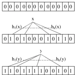
. For optimal performance, each of the k hash functions should be a member of the class of universal hash functions (Koloniari, Pitoura, 2003). That is, these hash functions map each item in the universe to a random number uniform over the range {1 … m}. (In practice, reasonable hash functions appear to behave adequately, e.g. MD5) Bloom filter works as follows (This is illustrated in Figure 1). To store an element x ∈ S, the bits hi(x) are set to 1 for

1

≤

i

≤

k

. A location can be set to 1 multiple times, but only the first change has an effect. To check if an element y is in S, one simply checks whether all hi(y) are set to 1. If not, then clearly y is not a member of S. However, if all hi(y) are set to 1, we cannot infer that

element y is definitely in S. It is possible that by coincidence h1(y),…,hk(y) are all set to 1. This situation is called false–positive and the probability that this occurs is called false-positive rate. Hence a Bloom filter does not yield a false negative but may yield a false positive, where it suggests that an element y is in S even though it is not. Figure 1 provides an example.

Figure 1. Illustration of bloom filter

The false-positive rate is a function of the length of the filter and the number of items stored in it. The smaller the filter, and the more items it contains, the greater that will give a false positive. For many applications, false positives may be acceptable as long as their probability is sufficiently small. The probability of a false positive, or the false positive rate

f

, can be calculated in a straightforward fashion, given our assumption that hash functions are perfectly random. It is given in (Bloom, 1970) and ( Mullin, 1983).

k

p

f

≈

(

1

−

)

,

p

=

e

−kn/m (1)

The parameters

k

and

m

should be chosen such that the probability of false positive is acceptable. The minimum is achieved for

k

=

ln

2

×

m

/

n

hash functions. However,

k

must be an integer and in practice a value less than optimal is usually chosen to reduce computational overhead. The computational overhead of each additional hash function is constant while the incremental benefit of adding a new hash function decreases after a certain threshold. The graph in Figure 2 shows the false positive rate

f

as a function of the number of bits allocated for each element, that is the ratio

m /

n

, for four values of

k

. The top curve is for the case of 7 hash functions. The bottom curve is for the optimum number of hash functions. It is clear that Bloom filters require very little storage per element at the slight risk of some false positives. For instance for a bit array 10 times larger than the number of entries, the probability of a false positive is 1.2% for 4 hash functions, and 0.9% for the optimum case of 5 hash functions. The probability of false positives can be easily decreased by allocating more memory.

0 0 0 0 0 0 0 0 0 0 0 0

0 1 0 1 0 0 0 1 0 1 1 0

1 1 0 1 1 1 1 0 0 1 0 1

y

h

1

(x) …….….….…h

k

(x)

x

h

1

(y) …….….……….h

k

(y)

Figure 2. False positive rate

3. Properties of Bloom Filters

• Since Bloom filters are bit-vectors it is possible to merge two or more of them by bitwise ORing to produce a conglomerate single merged one. For example, suppose we have sets S1 and S2 represented respectively by two Bloom filters

B

₁ and

B

₂, with the same number of bits and using the same number of hash functions. Then a Bloom filter

B

that represents the union

2 1

S

S

S

=

∪

of the two sets can be obtained by taking the OR of the two bit vectors of the original Bloom filters, that is

B

=

B

₁

∨

B

₂. The merged filter will recognize any inputs recognized by any of its ancestors.

• Bloom filters can easily be halved in size. Suppose the size of the filter is a power of 2. To half the size of the filter, just OR the first and second halves together. When hashing, the high order bit can be masked.

• Bloom filter bit arrays are robust in the presence of errors. If part of the array was corrupted, merely substitute all 1’s for the corrupted bits. This will slightly increase the false positives rate, but no false negatives will be introduced.

4. Compressed Bloom Filters

Compressing Bloom filter improves performance when the Bloom filter is passed as a message between nodes, particularly when information must be transmitted repeatedly, and its transmission size is a limiting factor. For example, Bloom filters have been suggested as a means for sharing Web cache information. In this setting, proxies do not share the exact contents of their caches, but instead periodically broadcast Bloom filters representing their cache. However, if we choose the optimal value for k to minimize the false probability as calculated above, then

p

=

1

/

2

. Under our assumption of independent random hash functions, the bit array is essentially a random string of 0's and 1's, with each entry being 0 or 1 with probability 1/2. It would therefore seem that no gain in compression when sending such Bloom filters.

On the other hand, large sparse Bloom Filters can be greatly compressed (Mitzenmacher, 2001). Theoretically, an m-bit filter can be compressed to

)

( p

mH

bits where p is the probability that a bit in the filter is 0 and

( )

p

p

p

(

p

)

(

p

)

H

=

−

log

₂

−

1

−

log

₂

1

−

is the entropy function. For sufficiently large filters, arithmetic coding guarantees close to optimal compression, so if p is small enough, H(p) is much smaller than 1, and significant savings in the transmission size can be achieved.

Hence, by using such compressed Bloom filters, proxies can reduce the number of bits broadcast, the false positive rate, and/or the amount of computation per lookup. The cost is the processing time for compression and decompression, which usually uses simple arithmetic coding, and more memory use at the proxies, which utilizes the larger sparser array of uncompressed form of the Bloom filter.

5. Counting Bloom Filters

If the set of elements is changing over time then insertions and deletions in the Bloom filter become important. Inserting elements into a Bloom filter is easy; hash the element k times and set the bits to 1. However, deletion by reversing this process, i.e. hashing the element to be deleted k times and set the corresponding bits to 0, is not possible. This is because we may be setting a location to 0 that is hashed to by some other element in the set, and the resultant Bloom filter is no longer correctly reflects all elements in the set.

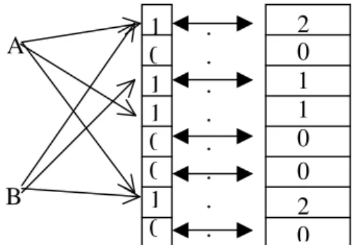
To avoid this problem, counting Bloom filter was introduced as an extension to Bloom filters (Czerwinski at al., 1999). Here, each entry in the Bloom filter is not a single bit but instead a small counter. When an item is inserted, the corresponding counters are incremented; and when an item is deleted, the corresponding counters are decremented (see Figure 3.). To avoid counter overflow, sufficiently large counters can be used. However, analysis from ( Fan, Cao, Almeida Broder, 2000) reveals that 4 bits per counter should be sufficient for most applications.

Figure 3. Incrementing/decrementing counters

6. Multi-level Bloom Filters

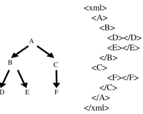
Traditional Bloom filters can be extended to be used on hierarchical documents. Koloniari et al introduced extensions to Bloom filters based on two alternative ways of hashing XML trees to support path expressions. They called these filters: ‘Breadth Bloom Filter’ (BBF), and ‘Depth Bloom Filter’ (DBF).

1

0

1

1

0

0

1

0

2

0

1

1

0

0

2

0

A

B

.

.

.

.

.

.

.

.

Figure 4. Multi level bloomfilters 6.1. Breadth Bloom filter (BBF)

Let T be an XML tree with j levels, with 1 as the root level. The Breadth Bloom Filter (BBF) for an XML tree T with j levels is a set of Bloom filters {BBF0, BBF1, BBF2, …, BBFi},

i

≤

j

. There is one Bloom filter, denoted BBFi, for each level i of the tree. In each BBFi, we insert the elements of all nodes at level i. To improve performance, we construct an additional Bloom filter denoted BBF0. In this Bloom filter, we insert all elements that appear in any node of the tree. For example, the BBF for the XML tree in Figure 4 is a set of four Bloom filters in Figure 5.

Note that the BBFis are not necessarily of the same size. In particular, since the number of nodes and thus keys that are inserted in each BBFi (i > 0) increases at each level of the tree, we analogously increase the size of each BBFi. However, for equal size BBFis, BBF0 is the logical OR of all BBFis,

1

≤

i

≤

j

.

The procedure that checks whether a BBF matches a query distinguishes between path queries starting from the root and partial path queries. In both cases, first we check whether all elements in the query appear in BBF0. Only if we have a match for all elements, we proceed by examining the structure of the path. For a root query /a1/a2/…/ap, (e.g. A/B/D) every level i from 1 to p of the filter is checked for the corresponding ai. The algorithm succeeds, if we have a match for all elements. For a partial path query, for every level i of the filter, the first element of the path is checked. If there is a match, the next level is checked for the next element and the procedure continues until either the whole path is matched or there is a miss. If there is a miss, the procedure repeats for level i + 1. For paths with the ancestor-descendant axis (e.g. A//D), the path is split at the //, and the sub-paths are processed. All matches are stored and compared to determine whether there is a match for the whole path.

BBF0 1 1 1 1 1 0 1 0 1 1 1 1 BBF1 1 0 0 0 1 0 1 0 0 0 0 0 BBF2 0 1 1 1 1 0 0 0 1 0 0 1 BBF3 0 0 0 1 0 0 1 0 0 1 1 1

Figure 5. The BBF for the XML tree in Figure1

C B A D E F <xml> <A> <B> <D></D> <E></E> </B> <C> <F></F> </C> </A> </xml> A B∪C A∪B∪C∪D∪E∪F D∪_E∪_F

6.2. Depth Bloom filters (DBF)

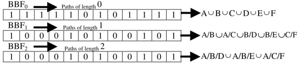
This provides an alternative way to summarize XML trees. Here different Bloom filters are used to hash paths of different lengths. The Depth Bloom Filter (DBF) for an XML tree T with j levels is a set of Bloom filters {DBF0, DBF1, DBF2, …, DBF i-1}, There is one Bloom filter, denoted DBFi, for each path of the tree with length i (i.e., a path of i + 1 nodes), where we insert all paths of length i. For example, the DBF for the XML tree in Figure 4 is a set of three Bloom filters in Figure 6. Note that we insert paths as a whole, we do not hash each element of the path separately; instead, we hash their concatenation. We use a different notation for paths starting from the root. This is not shown in Figure 6 for ease of presentation. Regarding the size of the filters, as opposed to BBF, all DBFis have the same size, since the number of paths of different lengths is of the same order. The procedure, that checks whether a DBF matches a path query, first checks whether all elements in the path expression appear in DBF0. If this is the case, we continue treating both root and partial paths queries the same. For a query of length p, every sub-path of the query from length 2 to p is checked at the corresponding level. If any of the sub-paths does not exist, the algorithm returns a miss. For paths that include the ancestor-descendant axis //, the path is split at the // and the resulting sub-paths are checked. If we have a match for all sub-paths the algorithm succeeds, else we have a miss.

BBF0 Paths of length 0 1 1 1 1 1 0 1 0 1 1 1 1 BBF1 Paths of length 1 1 0 0 0 1 0 1 0 0 1 0 1 BBF2 Paths of length 2 1 0 0 0 1 0 1 0 0 1 0 1

Figure 6. The DBF for the XML tree in Figure1

7. False Positives

The probability of false positives depends on the number k of hash functions we use, the number n of elements we index, and the size m of the Bloom filter. The formula that gives this probability f for standard Bloom filters is (Carter, Wegman, 1979):

f (1 –e kn/m ₎k ₍₂₎

Using multi-level Bloom filters, a new kind of false positive appears. Consider the

tree of Figure 1 and the path query /A/C/D. For BBFs, we have a match for C at BBF2 and for D at BBF3; thus we falsely deduce that the path exists. The probability for such a false positive is strongly dependent on the degree of the tree. For DBFs, we have a type of false positive that refers to queries that contain the // axis. Consider the paths a/b/c/d/ and m/n. For the query a/b//m/n, we split it to a/b and m/n. Both of these paths belong to the filter, so the filter would indicate a false match. A full analysis of false-positive rate for multi-level Bloom filters can be found in (Koloniari, Pitoura, 2003).

8. Samples of Applications

The following are samples of Bloom filter network applications. More applications can be found in ( Brodery, Mitzenmacherz, 2002) and (Chang, Feng, Wu-chang Li,

Kang, 2004). A/B∪A/C∪B/D∪B/E∪C/F

A/B/D∪A/B/E∪A/C/F A∪B∪C∪D∪E∪F

8.1. Distributed Caching

Fan, Cao, Almeida, and Broder describe Summary Cache, which uses Bloom filters for Web cache sharing [Fan, Cao, Almeida, Broder, 2000). In their setup, proxies cooperate in the following way: on a cache miss, a proxy attempts to determine if another proxy cache holds the desired Web page. If so, a request is made to that proxy rather than trying to obtain that page from the Internet. For such a scheme to be effective, proxies must know the contents of other proxy caches. In Summary Cache, to reduce message traffic proxies do not transfer URL lists corresponding to the exact contents of their caches, but instead periodically broadcast Bloom filters that represent the contents of their cache. If a proxy wishes to determine if another proxy has a page in its cache, it checks the appropriate Bloom filter. In the case of a false positive, a proxy may request a page from another proxy, only to find that that proxy does not actually have that page cached. In that case, some additional delay has been incurred. In this setting, false positives and false negatives may occur even without a Bloom filter, since the cache contents may change between periodic updates. The small additional chance of a false positive introduced by using a Bloom filter is greatly outweighed by the significant reduction in network traffic achieved by using the compact Bloom filter instead of sending the full list of cache contents. This technique is used in the open source Web proxy cache Squid, where the Bloom filters are referred to as Cache Digests (Rousskov, Wessels, 1998). Since cache contents are changing frequently (Fan, Cao, Almeida, Broder, 2000) suggests that caches use a counting Bloom filter to track their own cache contents, and broadcast the corresponding standard Bloom filter to the other proxies. The alternative would be to construct a new Bloom filter from scratch whenever an update is sent; using the counting Bloom filter both reduces and amortizes this cost. Using delta compression and compressed Bloom filters, as described in (Mitzenmacher, 2001), can yield a further reduction in the number of bits transmitted.

8.2. P2P/Overlay Networks

Peer-to-peer applications are a natural place to use Bloom filters, as collaborating peers may need to send each other lists of URLs, packets, or object identifiers. As an example of peer-to-peer application of Bloom filters is due to (Marais and Bharat, 1997) in the context of a desktop web browsing assistant called Vistabar. Cooperative users of Vistabar store annotations and comments about the web pages they visited in a central repository. Conversely they see these comments whenever they load an annotated page. Rather than make a request for each URL encountered, Vistabar periodically downloads a Bloom filter corresponding to all annotated URLs.

8.3. A Basic Routing Protocol

A general framework that highlights the main idea of resource routing protocols was described by Czerwinski et al. as part of their architecture for a resource discovery service (Czerwinski et al,1999). Suppose that we have a network in the form of a rooted tree, with nodes holding resources. Resource requests starting inside the tree head toward the root. Each node keeps a unified list of resources that it holds or that are reachable through any of its children, as well as individual lists of resources for it and each child. When a node receives a request for a resource, it checks its unified list to make sure it has a way of routing that request to the resource. If it does, it checks the individual lists to find how to route the request toward the proper node; otherwise, it passes the request further up the tree toward the root. This rather straightforward routing protocol becomes more interesting if the resource lists are

represented by Bloom filters. The property that a union of Bloom filters can be obtained by ORing the corresponding individual Bloom filters allows easy creation of unified resource lists. False positives in this situation may cause a routing request to go down an incorrect path. In such a case backtracking up the tree may be necessary, or a slower but safer routing mechanism may be used as a back-up. Several recent papers utilize a resource routing mechanism of this form.

8.4. Geographic Routing

Hsiao suggests using the type of routing in for a geographic routing system for mobile computers (Hsiao, 2001). For convenience, suppose that the geographic space is a square region that is recursively subdivided into smaller squares, each one-fourth the size of the previous level. That is, each parent square is broken into four children squares, giving a natural implicit tree hierarchy. If the smallest square subregions have size 1 and the size of the original square is

k

, there will be

1

log

₂

k

+

levels in this recursive structure. For the geographic routing scheme, each node contains a Bloom filter representing the list of mobile hosts reachable through itself or through its three siblings at each level. Using these filters, a source finds the level corresponding to the smallest geographic region that contains it and the destination, and then forwards a message to the centre of the region corresponding to the sibling that the destination node currently resides in. Intermediate nodes forward the message appropriately, recursing down the implicit tree until the destination is reached. Distributed hashing has also been proposed as a means of accomplished geographic routing (Li et al 2000). So for both P2P network and geographic routing, Bloom filters have been suggested as a possible alternative to distributed hashing that may prove better for systems of intermediate size.

8.5. Measurement Infrastructure

A growing problem for networks is how to provide a reasonable measurement infrastructure. How many packets from a given flow pass through a router? Has a packet from this source passed through this router recently? The challenge in coping with such questions lies in the tremendous amounts of data being processed, making complete measurement extremely expensive. Because of their succinctness, Bloom filters may be useful for many such problems, such as IP traceback described below. If one wanted to trace the route a packet took in a network, one way of doing it would be to have each router in the network record every packet that it forwards. Then each router could be queried to determine whether it forwarded the given packet, allowing the route of the packet to be traced backward from its destination. Such a scheme would allow malicious packets to be traced back along uncorrupted routers in order to find their source. Snoeren et al. (2001) suggest this approach with the addition of using Bloom filters in order to reduce the amount of information that needs to be stored in order summarize the set of packets seen, as part of their Source Path Isolation Engine (SPIE). A false positive in this setting means that a router mistakenly identifies a packet as having been seen. When attempting to trace back the reverse path of a packet, a false positive would lead to a branching, giving multiple possible paths. A low false positive rate would keep the branching small and hence the number of possible paths small as well. Of course to make such a scheme practical the authors gave careful consideration to how much information to store and when to discard stale information.

References

BLOOM, B. (1970). Space/time tradeoffs in hash coding with allowable errors.

Communications of the ACM, 13(7).

BRODERY, A. & MITZENMACHERZ, M. (2002). Network applications of Bloom Filters : a survey. Proceedings of 40th _{Annual Allerton Conference. Also}

available at <http://www.eecs.harvard.edu/_michaelm>

BYERS, J., CONSIDINE, J., MITZENMACHER, M., & ROST, S. (2002).

Informed content delivery across adaptive overly networks. Proceedings of ACM

SIGCOMM 2002, pp. 47-60.

CARTER, L., & WEGMAN, M. (1979). Universal classes of hash functions.

Journal of Computer and System Sciences, pp. 143-154. CS223 Final Project Report.

CHANG, F., FENG, W. & LI, K. (2004). Approximate caches for packet classification NSF Grant EIA-0130344, IEEE INFOCOM 2004.

CZERWINSKI, S., ZHAO, B.Y., HODES, T., JOSEPH, A.D., & KATZ, R. (1999). An architecture for a secure service discovery service. Proceedings of

MobiCom-99, pp. 24-35.

DHARMAPURIKAR, S., KRISHNAMURTHY, P., & TAYLOR, D. (2003). Longest prefix matching using Bloom Filters. Proceedings of the ACM

SIGCOMM, pp. 201-212.

FAN, L., P. CAO, J. ALMEIDA, & BRODER, A. Z. (2000). Summary cache : a scalable wide-area web cache sharing protocol. IEEE/ACM Transactions on

Networking, 8(3), pp. 281-293.

FELDMANN, A., & MUTHUKRISHNAN, S. (2000). Tradeoffs for packet classification, IEEE INFOCOM, 2000.

FENG, W., KANDLUR, D., SAHA D., SHIN, K., BLUE (1999). A new class of

active queue management algorithms, U. Michigan CSE-TR-387-99.

FENG, W. & KANDLUR, D.D. (2001). Stochastic fair blue : a queue management algorithm for enforcing fairness. Proceedings of IEEE INFOCOM 2001.

HSIAO, P. & HUANG, J. (2001). Geographical region summary service for wireless routing. MobiHoc 2001, Long Beach, CA, USA, pp. 263-266. Also available at <http://www.eecs.harvard.edu/~shawn/papers/courses/cs223_ final.pdf> as

CS223 Final Project Report.

HSIAO, P (2001). Geographical region summary service for geographical routing.

Mobile Computing and Communications Review, 5(4), pp. 25-39.

IAMNITCHI, A., RIPEANU, M. & FOSTER, I. (2002). Locating data in (Small-World?) peer-to-peer scientific collaborations. 1st _{International Workshop on}

Peer-to-Peer Systems IPTPS 2002. Also available at

http://arxiv.org/abs/cs/0209031.

KOLONIARI, G. & PITOURA, E. (2003). Bloom-based filters for hierarchical data.

5th _{Workshop on Distributed Data Structures and Algorithms (WDAS’03).}

. (2004). Filters for XML-based service discovery in pervasive computing. The Computer Journal, 47(4). Oxford University Press

for the BCS.

KUMAR, A. & LI, L. (2003). Space-code Bloom Filter for efficient traffic flow measurement. IMC’03 2003, Miami Beach, Florida, USA. Also available at: http://www.imconf.net/imc-2003/papers/p312-kumar1.pdf.

LI, J. & JANNOTTI, J. & DE COUTO, D & KARGER, D. & MORRIS, R. (2000). A scalable location service for geographic ad-hoc routing. Proceedings

MARAIS, H. & BHARAT, K. (1997). Supporting cooperative and personal surfing with a desktop assistant. In ACM Symposium on User Interface Software and Technology, pp. 129-138

MITZENMACHER, M. (2001). Compressed Bloom Filters. Proceedings of the 20th

ACM SIGACT Symposium on Principles of Distributed Computing (PODC 2001).

. (2001). Compressed bloom filters. Proceedings of the 20th

ACM SIGACT- SIGOPS Symposium on Principles of Distributed Computing, pp.

144-150.

MULLIN, J.K. (1983). A Second look at Bloom Filters. Communications of the

ACM, 26(8).

. (1990). Optimal semijoins for distributed database systems. IEEE

Transactions on Software Engineering, 16(5).

Passive measurement and analysis project, National Laboratory for Applied Network Research (NLANR). Available at http://pma.nlanr.net/Traces/Traces/ REYNOLDS, P. AND VAHDAT, A. (2003). Efficient Peer-to-peer keyword

searching. Middleware 2003, Rio de Janeiro Brazil, pp. 21-40. Also available at http://issg.cs.duke.edu/search/.

RIVEST, R. (1991). THE MD5 Message-Digest Algorithm. RFC1321.

ROUSSKOV, A & WESSELS, D (1998). Cache digests. Computer Networks and

ISDN Systems, 30(22-23), pp. 2155-2168.

SANCHEZ, L., MILLIKEN,W., SNOEREN, A.,TCHAKOUNTIO, F., JONES, C.,KENT, S.,PARTRIDGE,C., & STRAYER, W. (2001). Hardware support for a hash-based IP traceback. Proceedings of the 2nd _{DARPA Information}

Survivability Conference and Exposition.

SNOEREN, A. C., PARTRIDGE, L. A. SANCHEZ, C. E. JONES, F. TCHAKOUNTIO, S. T. KENT, & STRAYER, W. T. (2001). Hash-Based IP traceback. Proceedings of the ACM SIGCOMM 2001 Conference