LONG TERM IMPACT OF FINANCIAL SYSTEM ON IMPORT
DEMAND FOR TURKEY
FİNANSAL SİSTEMİN İTHALAT TALEBİ ÜZERİNDEKİ UZUN DÖNEM ETKİSİ: TÜRKİYE ÖRNEĞİ
Uğur ADIGÜZEL
(1), Tayfur BAYAT
(2), Selim KAYHAN
(3) (1, 3)Bozok Üniversitesi İİBF, (2)İnönü Üniversitesi İİBF(1)[email protected], (2)[email protected], (3)[email protected] ABSTRACT: In this study, we aim to analyze whether a shock in a component of the
financial system affect import demand on the long run. In this regard, we include components of financial system into the import demand function and employ long run SVAR method. We analyze the eight period from the beginning of “Transition Program for Strengthening the Turkish Economy”.
We conclude that import demand responses affect positively a national cash flow shock. Relative prices shock affects import demand positively, as expected. There is a number of variables belonging to a financial system which induces import demand. According to results, the financial system influences the import demand and policymakers have to take into account the interaction between import demand and financial system in the policy-making process.
Keywords: Import Demand; Long-Rrun Structural VAR; Financial System
ÖZET: Çalışmada finansal sistemin uzun dönemde ithalat talebi üzerindeki etkisini
görmek amacıyla, finansal sistem bileşenleri ithalat talebi fonksiyonu içerisine yerleştirilmiştir. Bununla birlikte eleştiriler doğrultusunda ithalat talep fonksiyonu içerisinde gayri safi yurt içi hasıla yerine ulusal nakit akışı değişkeni kullanılmıştır. Çalışmada finansal sisteme ait bir değişkenin uzun dönemde ithalat talebi üzerindeki etkilerini görmek amacıyla uzun dönem yapısal VAR metodolojisi kullanılmıştır. Kullanılan veriler "Güçlü Ekonomiye Geçiş Programı"nın uygulanmaya başladığı tarihten itibaren günümüze sekiz yıllık dönemi kapsamaktadır.
Çalışma sonucunda ulusal nakit akışının ithalat talebi üzerinde pozitif bir etkisinin bulunduğu, göreceli fiyatların ise ithalat talebini beklendiği gibi uzun dönemde pozitif etkilediği görülmüştür. Finansal sisteme ait değişkenlerden bazılarının ise ithalat talebi üzerinde anlamlı etkilerinin olduğu sonucuna ulaşılmıştır. Sonuçlar politika yapıcılarının politika kararlarında bu etkileşimi dikkate almaları gerektiğini göstermektedir.
Anahtar Kelimeler: İthalat Talebi; Uzun Dönem Yapısal VAR; Finansal Sistem JEL Classification: E44; F41
1. Introduction
At the end of 20th century, globalization has become an important matter because of
evolution in communication and transportation technologies. Structures of financial markets and commercial transmission mechanism have changed in conjunction with globalization. The development of communication and transportation technologies have simplified to reach international market and to trade into there as well. In this
regard, globalization may be thought of as the integration of economies through capital flow, trade and information technology (Mubiru, 2003: 3).
Hereafter, an increase in international trade has had a major role on macroeconomic policies because of the fact that its effect on economy and interdependence of macroeconomic policies has increased between trading countries. Determinants of import and export have become important variables for both policymakers and economists. So, determining the components of export and import demand would help to control balance of payments and to give incentives to right sectors to support. A number of economists have studied to identify variables affecting import and have tried to construct an import demand function. In these studies, different variables are included into models and practiced several different kind of methodology in order to get robust stable import demand function. In this context Khan (1975) implied that marginal propensity to import is dependent on the composition of income, while Leamer and Stern (1970) emphasized that real GNP and relative price of import are explanatory variables used in total import demand analysis. In another study, Goldstein et al. (1980) connoted the indicators of import demand as importing country's level of income or real expenditure and the ratio of the price of imports to the price of domestic import substitutes. Faini et al. (1988) determined traditional import demand function by relating real imports (Mt) to real income (Yt) and ratio of import
prices (PtM) to domestic prices (PtD) which was estimated for fifty countries as follows:
tM tD
tt
t b b Y b P P v
M ln ln /
ln 0 1 2 (1)
where vt is an error term with standard properties. Although equation built above could
explain some portion of import demand, undertaken examination for most of countries, Faini et al. (1988) found import demand function unstable.
Import demand function was predicted by Shabbir and Mahmood (1991) for Pakistan, Carone (1996) for USA, Gregory and Hansen (1996) and Hamori and Matsubayashi (2001) for Japan, Dutta and Nasuriddin (1999) for Bangladesh, Tang and Nair (2002) for Malaysia, Tang (2002) for Indonesia, Chang et al. (2005) for South Korea. They analyzed import demand by using conventional variables such as income and relative prices. Although some of studies found significant results, a number of them found unstable and insignificant results for import demand.
To constitute stable and significant import demand function, authors have developed liberally models in their studies. Khan (1974) included import restrictions and tariffs as a proxy of import determinants. Murray and Ginman (1976) and Salas (1982) included import prices and domestic prices separately instead of ratio of import prices to domestic prices. Chu et al. (1983) used indicators of foreign exchange availability as a proxy for tend of government to impose import controls. Faini et al. (1988) focused on import controls to determine import demand also. Diewert and Morrison (1986) used producer oriented framework to model import/export demand and included domestic supply and labour demand to explain them.
Gumede (2000) examined import demand function by including exchange rates into equation. Narayan and Narayan (2005) built a model including relative prices, total consumption, investment expenditure and export expenditure variables to model a
stable import demand in a different way. Metha and Parikh (2005) included the index of non-tariff barrier for a spesific commodity group into equation. Dash (2005) added real exchange rate reserve of importer country into its import demand equation in his study.
Also there is a vast literature examining Turkish economy. One of them belongs to Kutlar and Simsek. Kutlar and Simsek (2003) examined import demand of the Turkish economy between 1987 and 2000 by using Johansen cointegration analysis method. Gul and Ekinci (2006) and Barisik and Demircioglu (2006) analyzed 1990 - 2006 and 1980 - 2001 periods, respectively. Kutlar and Simsek (2003) and Barisik and Demircioglu (2006) found long term relationship between import, export and real exchange rate. Gul and Ekinci (2006) found no relationship between them contrary to findings of Kutlar and Simsek (2003). Kalyoncu (2006) and Bayraktutan and Bıdırdı (2010) implied that real income is the main indicator of import demand in Turkey. Aydin et. al (2004) and Karagöz and Doğan (2005) are other studies examined Turkish import demand.
As indicated by Mubiru (2003), domestic financial markets participated into the international financial system as result of globalization process. Besides increasing volume of international trade, globalizing financial markets brings to mind question that whether developing financial markets have any effect on important demand. In initial study of Leamer and Stern (1970), credit was neglected to import and export demand function. This variable is meant to indicate the availability and terms at which credit is provided for the financing of imports. Such a variable will play important role especially in linking the current and capital accounts of the balance of payments (Leamer and Sterns, 1970: 16). They also emphasized that increasing interest in the capital account will surely provide a stimulus to increased examination of the effect of credit on imports and exports. An increase in financial system depth would provide alternatives for importing companies. A well built financial system would reduce risk-premium and it would cause decreasing costs. Better developed financial sectors have a comparative advantage in manufacturing industries (Deck, 2002: 107). According to Leamer and Sterns (1970), transaction volume in exchange market, stock market or total credit volume in banking sector is important indicators of financial system depth. Deck (2002) included development degree of financial system in his analysis about foreign trade structure and examined linkage between financial development and structure of trade balance by using data covering thirty years between 1966 and 1995 belonging 65 countries. He employed the Generalized Methods Moments (GMM) and concluded that there is a link between the level of financial development and the structure of international trade (Deck, 2002: 129).
In another study of Tang (2004), he tried to construct more stable (or long run) import demand function for the Japanese economy between years 1973 and 2000. In order to achieve this, he put financial variables into function and analyzed by using co-integration methodology. He used ARDL bounds test, Johansen's multivariate approach and error correction model. He concluded that financial variables and monetary policies have important effects on import demand function for Japan economy.
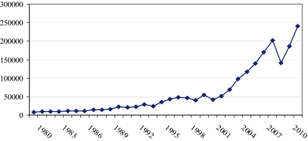
By the beginning of export-led growth regime in 1980, international trade volume of Turkey has started to increase gradually. Besides, increasing export, total amount of import has started to increase. It was only 8 billion US dollar in 1980 and it increased to 15 billion US Dollars in 1989. Increase has continued in 90's and it reached to 40 billion US Dollars in 1999. By the beginning of stabilization program named " Transition Program for Strengthening the Turkish Economy", after the financial crisis in 2001, development of economy has affected all sectors and quantity of import has accelerated in this era. Quantity of total import was 41 billion US Dollars in 2001 and it was more than 140 billion US Dollars at the end of 2009. Import amount by years is shown in figure 1. 0 50000 100000 150000 200000 250000 300000 1980 1983 1986 1989 1992 1995 1998 2001 2004 2007 2010
Figure 1. Import Amount by Years (Million US dollar)*
Financial system of Turkey has experienced structural change after financial crisis in 2001 also. In the stabilization program, government took regulatory decisions about the structure of Turkish financial system. One of the most important decisions was that the structure of state banks were aimed to regulate and governance of these banks ought to be improved. Another one was about stability of financial system and in this context, problems of wrecked banks existing in the Saving Insurance Deposit Fund (SIDF) ought to be solved in a short time. Also some regulations had to practice on private banking sector and to this end capital structure of private banks ought to be improved.
Accelerating import amount and re-structuring of financial system in 2000s provide room to re-examine import demand of Turkey. In this regard, we aim to re-construct import demand function of Turkey by including financial market to get long run import demand function and to see whether an evolution in financial market affected import demand of Turkey. The novelty of this paper is twofold. First of all, although the amount of export goods has increased in last decade, trade deficit is still an important problem for the Turkish economy because of high import volume. Re-examining the import demand and investigate whether a shock in financial system is effective on import demand are essential for the Turkish economy. In this regard, investigation of the interaction between variables would be useful for policy makers. Secondly, there is no study investigating the import demand of Turkey by including financial system components. In this context, this is the first study to our knowledge.
The rest of paper is organized as follows. In the second section of the study, we build up model and introduce data used in econometrical analysis. The third section is about empirical results and in the last section conclusions are presented.
2. Data and Methodology
In our study we examine data between years 2002 and 2009. Because, structural change in financial system experienced by the end of financial crisis in 2001. We take monthly data into account and it is obtained from the Central Bank of the Republic of Turkey official website. In order to analyze the effects of financial system on import demand, we use five variables belonging system and these are explained in Table 1. Xu (2002) indicates that conventional import demand equations generally regarded as statistics and its empirical specifications are often criticized as ad hoc. In order to derive tractable structural import demand equation, we use gross domestic product, government expenditures, total investments and export data to calculate national cash flow (ncf) as mentioned in Xu's (2002) study.
Another variable which we include into function is relative prices (rp). We can use real effective exchange rate in order to introduce relative prices because of similarities in definitions of relative prices and real effective exchange rate.† For this reason, we use real effective exchange rate in our analysis instead of relative prices. Lastly, we employ total import value of Turkey (m) as dependent variable of analysis. Details of data are given in the following table. In order to deseasonalize the variables, we use TRAMO/SEATS program and we deseasonalize NCF and M data.
Also we take natural logarithm of all variables. To see effects of each financial variable, we build up import demand function for each variable of financial system, respectively. So we analyze five different import demand function like in the study of Tang (2004) to see individual effects of financial variables on import demand. In this context, we connote models for each variable as follows:
Table 1. Data Set
Variables Explanation Source
m Import Value (TL) CBRT
ncf National Cash Flow (TL) (GDP - I - G – EX) CBRT rp ( Real Effective Exchange Rate Used) CBRT crd Total Credit Volume in Banking Sector (TL) CBRT imkb Istanbul Stock Exchange Transaction Volume (TL) CBRT exmar Exchange Market Transaction Volume ($) CBRT deprate Interest Rate of Deposits (%) CBRT
spr Share Prices (TL) CBRT '
)
,
,
,
(
t t t t tf
m
ncf
rp
crd
X
(2) ')
,
,
,
(
t t t t tf
m
ncf
rp
imkb
X
(3) ')
,
,
,
(
t t t t tf
m
ncf
rp
exmar
X
(4) ')
,
,
,
(
t t t t tf
m
ncf
rp
deprate
X
(5) ')
,
,
,
(
t t t t tf
m
ncf
rp
spr
X
(6)† For detailed information, see Nilsson (1999).
The variables included into model can be written in a system of simultaneous equations represented in vector form like in equation (7) as follows.
t t
t B L y C
Ay ( ) 1 (7)
yt is a vector of endogenous variables, y t-1 is a vector of their lagged values and
t iswhite noise vector of the disturbance terms for each variable. This disturbance term captures any exogenous factors in the model. A contains the structural parameters of the contemporaneous endogenous variables and it is a nxn square matrix. C is also nxn square matrix and contains the contemporaneous response of the variables to the disturbances and innovations. B(L) is a sth degree matrix polynomial in the lag operator L, where s is the number of lagged periods used in the model.
There is a problem about representation with equation (7), because the coefficients in the matrices are unknown and identifying model is not possible in this form. But it is possible to transform equation into reduced form model to obtain standard VAR representation.
t t
t D L y e
y ( ) 1 (8)
In equation (8), D(L) equals A-1B(L) and et represents A-1C.ε The error terms et are
linear combinations of the uncorrelated shocks (εt) such that each individual error term
is serially correlated with a zero mean and a constant variance. The matrix Σ is the
variance/covariance of et of the standart VAR. Theσ2is the variance and σ ij are the
covariance terms where each (1/ )
1
T
T e e
ij t it jt and
matrix is represented as follows,
2 2 1 2 2 2 21 1 12 2 1 ... ... ... ... .. ... ... ... ... ... ... ... ... ... ... ... n n n n n (9)In this matrix Σ, there are (n2-n)/2 number of restrictions requried to identify the
system. Traditional VAR methodology proposes the identification restrictions based upon on a recursive structure known as Cholesky decomposition (Ioannidis et al., 1995: 256). Cholesky decomposition implies that first variable responds only to its own exogenous shock, the second variable responds to the first variable and its own exogenous shock. This structure gives lower triangular matrix form.
Because of its sensitiveness to ordering of variables, Cholesky decomposition methodology has some critiques from economic profession. These criticisms led to the development of the SVAR approach (McCoy, 1997: 6). The SVAR approach, as advocated by Sims (1980), Bernanke (1986) and Blanchard and Watson (1986), estimates the structural parameters by imposing contemporaneous structural restrictions based on economic theory.
McCoy (1997) summed up SVAR methodology as a standard VAR where the restrictions needed for identification of the underlying structural model are provided
by economic theory which can be either contemporaneous or long run restrictions depending on whether economic theory suggests. He implied that long-run empirical analysis can be more attractive for economists because there is more agreement on the long-run properties of economic theory.
Blanchard and Quah (1989) structured an alternative SVAR approach and considered the shocks as having permanent effects. This would imply that variables are non-stationary since the shocks continue to accumulate through time given they are permanent. The presence of unit roots in the variables can give rise to spurious regression if the VAR is estimated in levels (McCoy, 1997: 7). For this reason it is necessary to use first difference of variables in the case of shocks have permanent effects.
In the case where the shocks are temporary effects on the variables the restrictions are imposed on the contemporaneous elements contained in A, C and ∑. In contrast where the shocks are assumed to have permanent effects, the restrictions are imposed on the long-run multipliers in the impulse response functions, which in effect involves restrictions on D(L) (McCoy, 1997: 8). The long-run multipliers can be derived from a moving average representation of equation (7) as below:
I D L L
et
I D L L
A C t L t y ( ) 1 ( ) 1 1 ( ) (10) The term ( ) 0 i L iLi , where each
i is the impact of changes in the shocks ε t as reflected in the response of the variable yt+i. These
i are the impact multipliersand the sum of these responses to infinity is the long run multiplier of each variable. The set of these multipliers is the impulse response function.
We construct our restrictions as follows. First of all, we try to separate contemporaneous shocks and permanent shocks from each other. To do so, we assume that import demand is a function of innovations upon itself and we expect that import demand would increase through the positive shocks upon itself. This assumption provides three restrictions. Another assumption is that national cash flow will be affected by only an innovation in import demand and an innovation upon itself. Because import quantity exists in the definition of national cash flow and this provides two more restriction. The third identifying assumption is that relative prices would be contingent upon the structural innovations on import demand, national cash flow and itself. This assumption provide us the last restriction on D(L). The representation of D(L) is as follows, z11 0 0 0 z21 z22 0 0 D(L) = z31 z32 z33 0 z41 z42 z43 z44 (11)
After the identification of restrictions, next step is to determine impulse response function (IRF) that is employed to reflect the dynamic effect of each exogenous variable response to the individual unitary impulse from other variables. The IRF can explain the current and lagged effect over time of shocks in the error term (Liu et al., 2008: 243).
The variance decomposition is another test to understand dynamic relationship between variables in the VAR analysis. Variance decomposition gives information about dynamic structure of system. The main purpose of variance decomposition is to introduce effects of each random shock on prediction error variance for future periods (Ozgen and Guloglu, 2004: 9).
3. Empirical Results
In order to find the stationary of the series, or in other words whether they include roots or not, DF-GLS developed by Elliot, Rothenberg, Stock (1996) and KPSS unit root tests developed by Kwaitkowski, Phillips, Schmidt and Shin (1992) is used. In KPSS test that depends on Langrangean multiplier principle, different from the other unit root tests in literature, null hypothesis means trend stationary (average stationary) as it distinguishes series from deterministic trend (Ozgen and Guloglu, 2004: 14). DF-GLS tests, on the other hand, distinguish the series from the trend and eliminate the autocorrelation. Having an asymptotic distribution, when deterministic terms take place, this test gives better results compared to Dickey Fuller unit root test. (Ozgen and Guloglu, 2004: 16).
Table 2. Results of Kwiatkowski-Phillips-Schmidt-Shin (KPSS) Unit Root Test
Levels First Differences
Intercept* Trend+ Intercept ** Intercept* Trend+ Intercept **
m 0.9461 0.2479 0.1546 0.0375 ncf 1.0191 0.0318 0.2663 0.2347 rp 1.0467 0.1469 0.0544 0.0382 crd 1.2778 0.2520 0.4247 0.1183 imkb 1.1177 0.0601 0.0221 0.0136 deprate 0.8690 0.2715 0.5178 0.1372 spr 0.9992 0.1757 0.0694 0.0736 exmar 1.0319 0.2540 0.2470 0.0539
*The asymptotic critical values of LM statistic for intercept 0.739, 0.463 at the %1 and %5 levels.
** the asymptotic critical values of LM statistic for trend and intercept 0.216, 0.146 at the %1 and %5 levels. Table 3. Results of DF-GLS Unit Root Test
Levels First Differences
Without Trend* With Trend** Without Trend* With Trend** m -0.6120 [0] -1.9994 [0] -0.6124 [11] -1.3200 [11] ncf 3.5040 [11] -1.2255 [11] -0.2825 [11] -2.4791 [11] rp -0.8036 [2] -3.5667 [1] -5.9175 [0] -7.0377 [1] crd 2.2713 [1] -1.0127 [1] -4.5570 [0] -5.3507 [0] imkb -1.0307 [1] -5.4584 [0] -1.6478 [5] -12.7176 [0] deprate 0.1411 [1] -1.1662 [1] -5.8589 [0] -6.0658 [0] spr -0.1937 [1] -1.9610 [1] -6.5327 [0] -7.1071 [0] exmar -0.1540 [4] -3.2228 [0] -0.9475 [5] -10.7073 [0] * The asymptotic critical values for without trend -2.591, -1.944 at the %1 and %5 levels.
** The asymptotic critical values for with trend -3.602, -3.1772 at the %1 and %5 levels. The figures in parenthesis denote the number of lags in the tests that ensure white noise residuals. They were estimated through the Schwarz criterion.
Although KPSS and DF-GLS unit root tests have advantageous sides for each other, it has been observed that all the variables that were dealt with are not stable in grade values. Thus, when the first difference of the variables [I(1)] that were taken to analysis extent according to the fact that both test results are taken, it becomes stable. Dickey-Fuller type unit root tests generally tend to refuse the null hypothesis when there is a structural break. In this case, for a stationary series in reality, the tests tend to
accept the alternative hypothesis which defines that the series includes unit root (Perron, 1989: 1361). Lumsdaine-Papell (1999) and Lee-Strazicich (2003, 2004) tests are the instances for double structural break and endogenously determined tests. Lee-Strazicich (2003) test alternative hypothesis states the stationary of the trend. In other words, Lee -Strazicich (2003, 2004) unit root test helps to find two structural breaks (LM, Langrange Multiplier). Only Model A and C take place in Lee-Strazicich (2003) unit root tests. Model A gives the grade break and Model C gives both the grade and trend break. (Temurlenk and Oltulular, 2007: 4).
Model A;
k j t j t j t t t t K y t DU DT d y y 1 1 1 1 2 (12) Model C;
k j t j t j t t t t t t t y d DT DT DU DT DU t y K y 1 1 1 2 2 1 1 2 2 1 (13)Here, A is the first difference operator, ε tis the white noise disturbance term with
variance σ 2; and t=1,.. ..T is an index of time. The j t
y
terms on the right-hand side of equation (12) and (13) allow for serial correlation and ensure that the disturbance term is white noise. DUt, is an indicator dummy variable for a mean shift occurring attime TB and DTt are the corresponding trend shift variables, where; (Narayan and
Smyth, 2005: 1109- 1116). 1 0 0 t t t TB DU t TB otherwise DT t TB otherwise (14)
Table 4. Results of Lee-Strazicich Unit Root tests
Model A Model C
Min. t
stat. Break 1 Break 2 Min. t stat Break 1 Break 2
m -10.636 10.2004 (0)* [1.1921]** 08.2007 (0)* [0.8109]** -11.4847 08.2007 (0)* [4.5026]** 11.2007 (0)* [-3.7395]** ncf -10.760 02.2006 (0)* [-0.1519]** 06.2007 (0)* [-0.2204]** -11.5348 09.2007 (0)* [3.1367]** 02.2008 (0)* [-2.7382]** rp -10.248 02.2005 (0)* [0.5266]** 05.2007 (0)* [0.0119]** -11.4971 01.2008 (0)* [4.9460]** 04.2008 (0)* [-3.4921]** crd -10.797 06.2006 (0)* [-0.1926]** 11.2007 (0)* [-0.2317]** -11.4288 01.2008 (0)* [2.8263]** 06. 2008 (0)* [-2.1952]** imkb -2.5797 09.2005 (1)* [-1.0159]** 12.2006 (1)* [-0.4385]** -9.6718 12.2006 (0)* [2.8762]** 06.2008 (0)* [-8.5323]** deprate -4.8225 04.2004 (1)* [-0.2422]** 02.2007 (1)* [-0.6998]** -11.4396 06.2008 (0)* [1.5127]** 09.2008 (0)* [-3.2635]** spr -4.1471 10.2005 (1)* [2.0483]** 03.2007 (1)* [0.6833]** -11.0065 04.2008 (0)* [8.8627]** 08.2008 (0)* [-2.8782]** exmar -10.5961 09.2005 (0)* [-0.1108]** 02.2007 (0)* [-0.1868 ]** -12.2831 09.2008 (0)* [4.2719]** 02.2009 (0)* [-4.1526]** * Figures in parenthesis below the lag lengths are selected using the Akaike Information criterion.
** The critical values for the LeeStrazicich (2003) test is Model A : 4.545, 3.842 and 3.504; Model C: -5.823, -5.286 and -4.989 at the 1%, 5% and 10% levels.
Lee and Strazicich (2003, 2004) claim an endogenous two-break LM unit root test that allows for breaks under both null and alternative hypotheses. In addition, Lee- Strazicich's (2003, 2004) unit root test arrestingly the choice of lag length is crucial. Model A allows for two shifts in level and model C allows for two breaks in level and trend. The test results that were done on monthly series in Table 4 were meaningful in 1% and 5 % significance levels and the break dates were determined. As the assumption of the test requires, null hypothesis was denied and alternative hypothesis was accepted. Thus, in the years 2007 for import, 2008 for national cash flow, share price, interest rate on deposit, relative price and credit volume, 2006 for stock composite index, trading volume of foreign exchange market 2007 and 2008, the break was observed.
According to unit root test results all variables are I(1). To provide stationary condition of the reduced VAR model and ensure stationary in the case of shocks that have permanent effects as in Blanchard and Quah (1989), we include all variables in first differences in the analysis. Another important process in the VAR models is to select the optimal lag length. The most common and simple approach in selecting exact lag length is to re-estimate VAR model until the smallest Akaike Information Criterion (AIC) value is found. Because comparing two or more models, the model with the lowest AIC is preferred (Gujarati, 2004: 537). According to Asteriou (2005) the judgment of the optimal length should still take other factors into account: for example autocorrelation, heteroskedasticity, possible ARCH effects and normality of residuals.
a) Accumulated Response of m to m Shock b) Accumulated Response of m to ncf Shock
c) Accumulated Response of m to rp Shock d) Accumulated Response of m to crd Shock Figure 2. Impulse-Response Graphics of Model 1
We examine import demand functions including each financial variables separately and we find six lags for equation (1) including credit volume, three lags for equation (2) including stock market transaction volume, six lags for equation (3) including exchange market transaction volume (3) and three lags for equation (4) including deposit interest rate. In order to test stability of models, we control characteristic roots of the matrix coefficients if they have a modulus less than one. We use autocorrelation test and unit root graph to test lag structure and stability of the number of the lag length. Results conclude that all roots are less than one and no roots are out of the unit
circle. Also null hypothesis assuming that there is no correlation between error variances up to 12 lags was accepted in 1% confidence interval.
a) Acc. Response of m to m Shock b) Acc. Response of m to ncf Shock
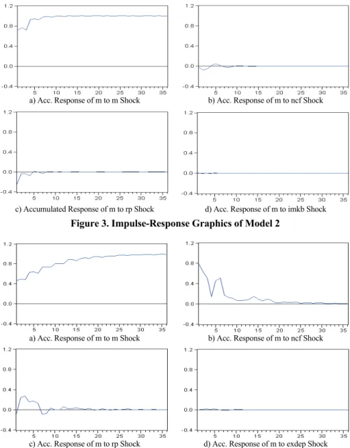
c) Accumulated Response of m to rp Shock d) Acc. Response of m to imkb Shock Figure 3. Impulse-Response Graphics of Model 2
a) Acc. Response of m to m Shock b) Acc. Response of m to ncf Shock
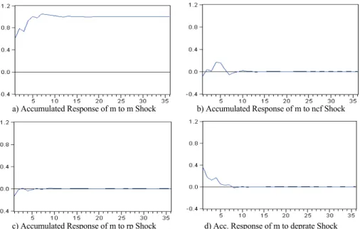
c) Acc. Response of m to rp Shock d) Acc. Response of m to exdep Shock Figure 4. Impulse-Response Graphics of Model 3
Figure 2 presents accumulated response of import demand to a structural shock in variables of model 1. Response of import demand to a positive innovation in national cash flow is positive. Effect of innovation decreases gradually in six months and then it dies out. A positive shock in relative prices affects import demand negatively in first impact. But it turns to positive after first month and dies out after fluctuated for a year. Response of import demand to a shock in total credit volume in the banking sector is valid for more than twenty months and it is positive along this period.
Figure 3 shows accumulated response of import demand to a shock in national cash flow, relative prices and stock market transaction volume. Results are summarized as follows. Including stock market transaction volume decreased responsiveness of import demand to national cash flow and relative prices. Response of import demand to a shock in national cash flow is positive after a quarter but the response is so small and finishes in a year unnecessarily. Response of the import demand to a shock in relative prices is negative and it turns positive fifth months after shock but it is unnecessarily small. According to results, an innovation in stock market transaction volume does not have any effect on import demand. It would not response to any shock in stock market.
Figure 4 presents impulse response function results for model (3) which includes exchange market transaction volume. According to results import demand responses positively to an innovation in national cash flow and relative prices. Effect of national cash flow innovation continues more than two years and effect of relative price innovation continues less than a year positively. According to results import demand does not response to a shock in exchange market transaction volume.
a) Accumulated Response of m to m Shock b) Accumulated Response of m to ncf Shock
c) Accumulated Response of m to rp Shock d) Acc. Response of m to deprate Shock Figure 5. Impulse-Response Graphics of Model 4
In the figure 5 accumulated response functions of variables belonging equation 4 is presented. According to results, responses of import demand to national cash flow and interest rate of deposit shocks are positive and both of them die out in a year. Effect of an innovation in relative price to import demand is unnecessarily small and negative. It already dies out in a quarter. Share prices are included in model 5 and accumulated response of import demand in the model is presented in figure 6. According to results, response of import demand is positive to a shock in national cash flow and it is effective more than a year. Although response is negative for relative prices and share prices in first impact, it turns to positive in the following months and continues more than a year.
In order to see explanatory power of variables to a shock in import demand, we use variance decomposition methodology. In model 1, national cash flow is the main explanatory variable of import demand shock. It can explain shock up to 56% during 36 months. While relative prices can explain shock up to 10%, credit volume in banking sector is another main explanatory and it explain 20% of variance in import demand. In model 2, explanation ability o national cash flow decreased although relative prices can explain variance up to 16%. In this model we have included stock market transaction volume and but according to variance decomposition results it has no ability to explain import demand variance. In model 3, national cash flow is the main variable to explain variance in import demand as in model 1. It explains variance up to 70%. Also share of relative prices increased up to 12%. Another variable belonging financial system, exchange market transaction volume does not have explanation ability in variance of import demand like stock market transaction volume.
a) Accumulated Response of m to m Shock b) Accumulated Response of m to ncf Shock
c) Accumulated Response of m to rp Shock d) Accumulated Response of m to spr Shock Figure 6. Impulse-Response Graphics of Model 5
By including interest rate of deposits into model 4, import demand was the main explanatory variable of a variance in itself and national cash flow and relative prices lost explanation abilities. Variable of financial system is also another important variable explain variance up to 22%. In the last model, we have included share prices into model. In this model national cash flow is the main explanatory variable as like in model 1 and 3. Relative prices are the other explanatory variable of variance in import demand up to 10%. Share prices have just a little explanation ability and it is not more than 3%.
4. Conclusion
In this study, we include important variables of financial system into import demand model to build up a stable import demand for the Turkish economy on the long-term and to understand effects of financial system on import demand. Accumulated response of import demand to an innovation in national cash flow is positive. But including variable belonging financial system affects response of import demand to national cash flow. It increases when total credit volume, interest rate and share prices
are included into model and it decreases when we include stock market transaction volume and exchange market transaction volume. We found that accumulated response of import demand to a shock in relative prices is negative in first impact then it turns to positive after a month with financial variables or without them. But it is clear that stock market volume and exchange market transaction volume affect responsiveness of import demand to relative prices negatively. When we examine variables belonging financial system, it is clear that total credit volume in the banking sector and interest rate of deposit have positive effects on import demand as Leamer and Stern (1970) emphasized in their study. Also share prices shock is effective on import demand and it increases when there is a positive shock on share prices. But response of import demand to total credit value is longer than the others and it continues more than two years significantly. We found also that import demand has no response to a shock in exchange market and stock market transaction volume.
We examine variance decomposition of import demand and we concluded that national cash flow can explain up to 70% of variance in import demand. While credit volume, interest rate and share prices increase explanation ability of national cash flow, other variables reduce it. Relative prices can explain a shock in import demand up to 15% and credit Explanation ability of relative prices is high and it can explain up to 15% percentage. Also variables of financial system affect it ability also like national cash flow. The most useful financial variable to explain variance of import demand is interest rate of deposits and it can explain up to 22%. Another one is total volume of credit in financial system and it can explain up to 20%. Another efficient variable is the share prices and but it can explain only up to 3%. Other two variable have no ability to explain variance of import demand in long term.
All these results indicate that including financial system into import demand might be effective to build a stable import demand function for Turkey. Effects of credit and interest rate on import demand correct Leamer and Stern's (1970) piece of advises about import demand structure. Results of analysis imply that effects of financial system on import demand must be taken into consideration by the Central Bank of the Republic of Turkey in policy making process.
References
ASTERIOU, D. (2005). Applied econometrics a modern approach using eviews and microfit. Revised Edition., Hempshire: Palgrave.
AYDIN, M.F., ÇIPLAK, U., YÜCEL, M.E. (2004). Export supply and import demand models for the Turkish economy. CBRT Research Department Working Paper, no. 04/09.
BARIŞIK, S., DEMÎRCİOĞLU, E. (2006). Türkiye'de döviz kuru rejimi, konvertibilite, ihracat- ithalat ilişkisi (1980-2001). Zonguldak Karaelmas Üniversitesi Sosyal Bilimler Dergisi, 2(3), 71 - 84. ss.
BAYRAKTUTAN, Y., BIDIRDI, H. (2010). Basic determinants of Turkish import (1989- 2004). Ege Academic Review, 10(1), 51 - 369. ss.
BERNANKE, B.S. (1986). Alternative explanations of the money- income correlation. Carnegie-Rochester Conference Series on Public Policy, 25, 49- 100. ss.
BLANCARH, O.J., QUAH, D. (1989). The dynamic effects of aggregate demand and supply disturbances. American Economic Review, 79, 655 - 73. ss.
BLANCHARD, O. J., WATSON, M.W. (1986). Are business cycles all alike? R. Gordon (ed) The American Business Cycle: Continuity and Change içinde. NBER and University of Chicago Press, Chicago: University of Chicago Press, 123 - 156. ss.
CARONE, G. (1996). Modeling the US demand for imports through cointegration and error correction. Journal of Policy Modeling, 18(1), 1 - 48. ss.
CHANG, T., HO, Y.H., HUANG, C.J. (2005). A reexamination of South Korea's aggregate import demand function: The bounds test analysis. Journal of Economic Development, 30(1), 119 - 128. ss.
CHU, K., HWA, E.C., KRISHNAMURTY, K. (1983). Export instability and adjustments of imports, capital flows and external reserves: A short-run dynamic model. D. Bigman and T. Taya (ed.), Exchange Rate and Trade Instability: Causes, Consequences, and Remedies içinde. Cambridge: Ballinger Publishing Co.
DASH, A.K. (2005). An Econometric Estimation of The Aggregate Import Demand Function for India. International Business Research Conference, Athens.
DECK, T. (2002). Financial develpoment and international trade is there a link?. Journal of International Economics, 57, 107 - 131. ss.
DIEWERT, E.W., MORRISON C.J. (1986). Export supply and import demand functions: a production theory approach. National Bureau of Economic Research Working Papers, no.2011.
DUTTA, D., NASIRUDDIN, A. (1999). An aggregate import demand function for Bangladesh: a cointegration approach. Applied Economics, 31(4), 465- 472. ss.
ELLIOT, G., ROTHENBERG, T.J., STOCK, J.H. (1996). Efficient tests for an autoregressive unit root. Econometrica, 64(4), 813 - 836. ss.
FAINI, R., PRITCHETT, L., CLAVIJO, F. (1988). Import demand in developing countries. The World Bank Working Papers, no. WPS 122.
GOLDSTEIN, M., KHAN, M.S., OFFICER, L.H. (1980). Prices of tradable and nontradable goods in the demand for total imports. The Review of Economics and Statistics, 62(2), pp. 190-199.
GREGORY, A.W., HANSEN, B.E. (1996). Residual-Based tests for cointegration in models with regime shifts. Journal of Econometrics, 70(1), 99 - 126. ss.
GUJARATI, D. (2004). Basic econometrics. Fourth Edition,, Chicago: McGraw-Hill Publications.
GUMEDE, V. (2000). Import performance and import demand functions for South Africa. TIPS Working Papers, no. 9.
GÜL, E., EKİNCİ, A. (2006). Türkiye'de reel döviz kuru ile ihracat ve ithalat arasındaki nedensellik ilişkisi: 1990- 2006. Dumlupınar Üniversitesi Sosyal Bilimler Dergisi, 16, 165- 190. ss.
HAMORI, S., MATSUBAYASHI, Y. (2001). An empirical analysis on the stability of Japan's aggregate import demand function. Japan and The World Economy, 13(2), 135- 144. ss. IOANNIDIS, C., LAWS, J., MATTHEWS, K., MORGAN, B. (1995). Business cycle analysis
and forecasting with a structural vector autoregression model for Wales. Journal of Forecasting, 14(3), 251 - 265. ss.
KALYONCU, H. (2006). An aggregate import demand function for Turkey: a cointegration analysis. The Indian Journal of Economics, 343, 1 - 11. ss.
KARAGÖZ, M., DOĞAN, Ç. (2005). Döviz kuru dış ticaret ilişkisi: Türkiye örneği. Firat University Journal of Social Science, 15(2), 219 - 228. ss.
KHAN, M.S. (1975). The structure and behaviour of imports of Venezuela. Review of Economics and Statistics, 57, 221- 224. ss.
KHAN, M.S. (1974). Import and export demand in developing countries. IMF Staff Papers, no. 21, 678 - 692. ss.
KUTLAR, A., ŞİMŞEK, M. (2003). Türkiye'de ithalat talebinin koentegrasyon analizi: 1987(I)- 2000(IV). Dokuz Eylül Universitesi İ.İ.B.F. Dergisi, 18(2), 65 - 82. ss.
KWIATKOWSKI, D., PHILLIPS, P.C.B., SCHMIDT, P., SHIN, Y. (1992). Testing the null hypothesis of stationarity against the alternative of a unit root: How sure are we that economic time series have a unit root? Journal of Econometrics, 54(1-3), 159 - 178. ss. LEAMER, E.E., STERN, R.M. (1970). Quantitative international economics. Boston: Allyn and
Bacon Inc.
LEE, J., STRAZICICH, M. (2004). Minimum LM unit root test with one structural breaks. Apalachian State University Working Papers, No 04-17.
LEE, J., STRAZICICH, M. (2003). Minimum LM unit root test with two structural breaks. Review of Economics and Statistics, 85(4), 1082 - 1089. ss.
LIU, C., LUO, Z.Q., MA, L., PICKEN, D. (2008). Identifying house price diffusion patterns among australian state capital cities. International Journal of Strategic Property Management, 12, 237 - 250. ss.
LUMSDAINE, R., PAPELL, D. (1999). Two structural breaks and the unit root hypothesis: New evidence about unemployment in Australia. Working Paper Series Victoria University Applied Economy Working Paper, no. 3/00.
MCCOY, D. (1997). How useful is structural VAR analysis for Irish economics. Eleventh Annual Conference of the Irish Economic Association, Athlone.
MEHTA, R., PARIKH, A. (2005). Impact of trade liberalization on import demands in India: A Panel Data Analysis for Commodity Groups. Applied Economics, 37, 1851- 1863. ss. MUBIRU, E. (2003). The effects of globalisation on trade - a speical focus on rural farmers in
Uganda. [Erişim Adresi]: http://www.global-poverty.org/policyAdvocacy/pahome2.5.nsf/ gereportsFAA90E89364586A388256E460083628B/$file/Edward. pdf, (Erişim Tarihi: 14.06.2010).
MURRAY, T., GINMAN, P.J. (1976). An empirical examination of the traditional aggregate import demand model. The Review of Economics and Statistics, 58(1),75- 80.
NARAYAN, S., NARAYAN, P.K. (2005). An empirical analysis of Fiji's import demand function. Journal of Economic Studies, 32(2), 158 - 168. ss.
NARAYAN, P., SMYTH, R. (2005). Electricity consumption, employment and real income in Australia evidence from multivariate Granger causality tests. Energy Policy, 33, 1109-1116. ss.
NILSSON, K. (1999). Alternative measures of the Swedish real effective exchange rate. National Institute of Economic Research Working Paper, No.68.
ÖZGEN, F.B., GÜLOĞLU, B. (2004). Türkiye'de iç borçların iktisadi etkilerinin VAR tekniğiyle analizi. ODTÜ Gelişme Dergisi, 31, 93 - 114. ss.
PERRON, P. (1989). Test consistency with varying sampling frequency. Princeton University Econometric Research Program Research Memorandum, no.345.
SALAS, J. (1982). Estimation of the structure and elasticities of mexican imports in the period 1961- 1979. Journal of Development Economics, 10, 297 - 311. ss.
SHABBIR, T., MAHMOOD, R. (1991). Structural change in the import demand function for Pakistan. Pakistan Development Review, 30(4), 1159 - 1166. ss.
SIMS, A.C. (1980). Macroeconomics and reality. Econometrica, 48(1), 1 - 48. ss.
TANG, T.C. (2002). Aggregate import demand behaviour for Indonesia: evidence from bounds testing approach. Journal of Economics and Management, 10(2),1-21.ss.
TANG, T.C. (2004). Does financial variable(s) explain the Japanese aggregate import demand? A cointegration analysis. Applied Economics Letters, 11(12), 775 - 780. ss.
TANG, T.C., NAIR, M. (2002). A Cointegration analysis of Malaysian import demand function: reassessment from the bound test. Applied Economics Letters, 9(5), 293- 296. ss.
TEMURLENK, S., OLTULULAR, S. (2007). Türkiye'nin temel makro ekonomik değişkenlerinin bütünleşme dereceleri üzerine bir araştırma. İnönü Üniversitesi Ekonometri ve İstatistik Kongresi, Malatya.
XU, X. (2002). The dynamic- optimizing approach to import demand: a structural model. Economics Letters, 74, 265 - 270. ss.