7
ISSN 2303-4521
PERIODICALS OF ENGINEERING AND NATURAL SCIENCES Vol. 2 No. 1 (2014)
Available online at: http://pen.ius.edu.ba
Mathematical modeling and analysis of tumor-immune system interaction by using
Lotka-Volterra predator-prey like model with piecewise constant arguments
Senol Kartal
Nevsehir Hacı Bektaş Veli University, Faculty of Science and Art, Department of Mathematics, 50300
Nevsehir, Turkey
Abstract
In this study, we present a Lotka-Volterra predator-prey like model for the interaction dynamics of tumor-immune system. The model consists of system of differential equations with piecewise constant arguments and based on the model of tumor growth constructed by Sarkar and Banerjee. The solutions of differential equations with piecewise constant arguments leads to system of difference equations. Sufficient conditions are obtained for the local and global asymptotic stability of a positive equilibrium point of the discrete system by using Schur-Cohn criterion and a Lyapunov function. In addition, we investigate periodic solutions of discrete system through Neimark-Sacker bifurcation and obtain a stable limit cycle which implies that tumor and immune system undergo oscillation.
Keywords: tumor growth, piecewise constant arguments, difference equation, stability
1. Introduction
Modeling tumor-immune interaction has attracted much attention in the last decades. This interaction is very complex and mathematical models can help to shape our understanding of dynamics this biological phenomenon. Most of the models consist of two main populations: tumor cells and effector cells such as hunting predator cells (Cytotoxic T lymphocytes) and resting predator cells (T-Helper cells) which are main struggle of immune system. Cytotoxic T lymphocytes (CTLs) responsible to kill tumor cells and resting predator cells account for to activity the native Cytotoxic T lymphocytes.
In order to describe tumor and effector cells interaction, many authors [1-16] have used Lotka-Volterra terms and logistic terms. While some of these models [1-9] consist of ordinary differential equations, the others [10-16] consist of delay differential equations. A familiar model included ordinary differential equations is constructed Kuznetsov and Taylor [1]. They have studied interaction between Cytotoxic T lymphocyte and immunogenic tumor and have obtained a threshold for the tumor growth. Kirschner and Panetta [2] have generalized this model to study the role of IL-2 in tumor dynamics. Another familiar tumor growth model has been proposed by Sarkar and Banerjee [3]. The model explains spontaneous tumor regression and progression under immunological activity.
On the other hand, there exists a discrete time delay in the mitosis phase (cell division phase) since tumor cells need a resting time for a proliferation. This biological phenomenon is explained much better by using delay differential equations instead of ordinary differential equations [10]. Therefore, many authors have considered delay differential equation included time delay factor for modeling tumor growth [10-16]. Sarkar and Banerjee [11] have constructed the model by using the time delay factor as follows:
where , and are the number of tumor, hunting and resting cells respectively.
Since stability and bifurcations analysis of delay differential equations is more difficult, numerical analysis may be needed for such equations. In study [17], Cooke and Györi show that differential equation with piecewise constant arguments can be used to obtain good approximate solution of delay differential equations on the infinite interval . Therefore, there has been great interest in studying differential equation with piecewise constant arguments which combine properties
8
of both differential and difference equations [18-26]. I. Ozturk et al. [18] have modeled bacteria population by using differential equation
which includes both continuous and discrete time for a bacteria population.
These types of models also allow us to describe both microscopic and macroscopic level events that occur simultaneously. For the tumor-immune system interactions, microscopic interaction refers proliferation and activation of tumor cells together with their competition while macroscopic interaction refers to cancer invasion and metastases [27]. When one considers the both microscopic level interaction which needs a discrete time and macroscopic level interaction which needs continuous time simultaneously, there are two events in a population: a continuity and discrete time. Modeling tumor growth using differential equation with piecewise constant arguments, Bozkurt [19] have considered a more general case of equation (2) as follows:
In the present paper, due to above biological facts, we replace the model (1) by adding piecewise constant arguments and get a system of differential equations
where denotes the integer part of , , and are the number of tumor, hunting and resting cells respectively. The parameter represents the growth rate and represents the maximum carrying capacity of tumor cells, is the growth rate and is the maximum carrying capacity of resting cells. The term is natural death of hunting cell. The competition term represents the loss of tumor cells due to encounter with hunting cells and represents the loss of hunting cells due to encounter with the tumor cells. The conversion rate from resting to hunting cells is represented parameter . There exist a discrete delay time in this conversion which is represented term . The term
represents growth of hunting T-cells and the term represents loss of resting cells.
2. Local and global stabilty analysis of the system
An integration of each equation in system (4) on an interval give us
where . If we solve each equations of system (5) and letting , we get a system of difference equations
In order to analysis system (6), we need to find positive equilibrium point of the system. If
then, positive equilibrium point of the system is determined as where
The linearized system of (6) about positive equilibrium point is where is
9
The characteristic equation of matrix is
Under the assumption
an eigenvalue of (10) are computed as .
Solving equation (11) with the fact and considering inequalities (7) and (8) we have
Thus, characteristic equation can be reduced second order equation
Now we can determine stability conditions of discrete system (6) through the equation (12).
Theorem 1. Let the positive equilibrium point of
system (6). Suppose that
is local asymptotic stable if
Proof. By using Schur-Cohn criterion, we obtain that is
locally asymptotically stable if and only if
The inequality (13) can be written
and
If we consider condition (7) and (8), it can be easily seen that (a) is always holds. From (b), we hold
which reveal
Under the condition
we can write This completes the proof.
Example 1. The parameter values which are taken from
[11] as ,
and the determined value
provide the conditions of Theorem 1. It can be seen that under the conditions given in Theorem 1, the positive equilibrium
point of system (6) is local asymptotic stable (see Figure 1a), where blue, red and black graphs represent , and population densities respectively.
Theorem 2. Let the conditions of Theorem 1 hold.
Moreover, assume that
. If
10
and , , then the positive equilibrium point is globally asymptotically stable.
Proof. Let
,
is a Lyapunov function with the positive equilibrium point . The change along the solutions of the system is
In addition, the change along the solutions of the first equation in system (6) is
. It can be seen that if ,
and then . Similarly, it can be shown that
Nn[Nn+1+Nn−2N]<0 and
. As a result, we obtain
.
Example 2. In order to try the conditions of Theorem 2,
initial conditions can be determined as , , and parameter values can be taken Example 1. Figure 1b shows that under the conditions given in Theorem 2 the positive equilibrium point is global asymptotic stable, where blue, red and black graphs represent , and population densities respectively.
Figure 1. The iteration solution of , and for different initial conditions.
3. Neimark-Sacker bifurcation analysis
In this section, we try to determine Neimark-Sacker bifurcation point of the system by using Schur-Cohn criterion that is given as follows.
Theorem A ([28]). A pair of complex conjugate roots of
lie on the unit circle and the other roots of all lie inside the unit circle if and only if
(a) and (b) (c)
If we rearranged the equation (10), characteristic equation can be obtained as the form (14) where
By using these results, bifurcation point can be determined as the following example.
Example 3. Solving equation c of Theorem A, we get
. Moreover, we have also
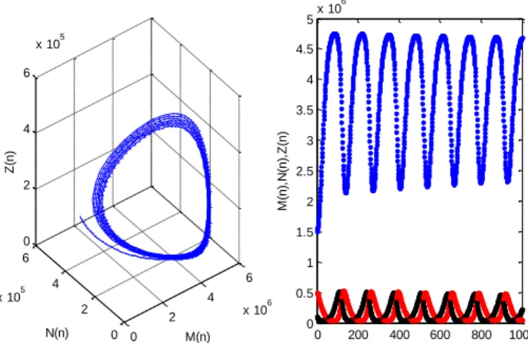
, ve for this point. Figure 2 shows that is the Neimark-Sacker bifurcation point of the system with the eigenvalues and
0.0544078i=1 where blue, red and black graphs represent , and population densities respectively. 0 200 400 600 800 6 6.5 7 7.5 8 8.5 9 9.5 10 10.5x 10 5 n M (n ), N (n ), Z (n ) 0 200 400 600 800 1000 0 1 2 3 4 5x 10 6 n M (n ), N (n ), Z (n ) b) a)
11
Figure 2. Neimark-Sacker bifurcation of system (6) for, where , , . The other parameters are taken Example 1. As seen in Figure 2, a stable limit cycle occurs at the bifurcation point as a result of Neimark-Sacker bifurcation. This result leads to stable periodic solutions around the positive equilibrium point. Determining bifurcation point is very important issue for the control of the tumor cell population. After the bifurcation point, tumor and immune system will exhibit unstable oscillatory behavior, thus resulting uncontrolled tumor growth. The solutions of the system at the point can be seen in Figure 3, where the
system has damped oscillation and the positive equilibrium point is local asymptotic stable. At the point , system (6) has unstable
oscillation and the positive equilibrium point is unstable (see Figure 4).
Finally, we can compare our theoretical results to the system (4) that is given in [11]. In study [11], a hopf bifurcation that is continuous case of Neimark-Sacker bifurcation is occurred around positive equilibrium point through stable limit cycle. Thus, we can say that bifurcation results of system (6) and system (4) are similar.
Figure 3. The iteration solution of the system for
. The other parameters and initial conditions
are the same as Figure 2.
Figure 4. The iteration solution of the system for
. The other parameters and initial conditions
are the same as Figure 2.
4. References
[1] V. A. Kuznetsov, I. A. Makalkin, M. A. Taylor et al., “Nonlinear dynamics of immunogenic tumors: parameter estimation and global bifurcation analysis,” Bulletin of Mathematical Biology, vol. 56, no. 2, pp. 295-321, 1994.
[2] D. Kirschner and J. C. Panetta, “Modeling immunotherapy of the tumor-immune interaction,”
Journal of Mathematical Biology, vol. 37, no. 3, pp. 235-252, 1998.
[3] R. R. Sarkar and S. Banerjee, “Cancer self remission and tumor stability- a stochastic approach,”
Mathematical Bioscience, vol. 196, no. 1, pp. 65-81,
2005.
[4] A. D. Onofrio, “A general framework for modeling tumor-immune system competition and immunotherapy: mathematical analysis and biomedical inferences,” Physica D-Nonlinear
Phenomena, vol. 208, no. 3-4, pp. 220-235, 2005.
[5] A. D. Onofrio, “Metamodeling tumor-immune system interaction, tumor evasion and immunotherapy,” Mathematical and Computer
Modelling, vol. 47, no. 5-6, pp. 614-637, 2008. [6] R. A. Gatenby, “Models of tumor-host interaction as
competing populations: implications for tumor biology and treatment,” Journal of Theoretical
Biology, vol. 176, no. 4, pp. 447-455, 1995.
[7] A. Merola, C. Cosentino and F. Amato, “An insight into tumor dormancy equilibrium via the analysis of its domain of attraction,” Biomedical Signal
Processing and Control, vol. 3, no. 3, pp. 212-219, 2008.
[8] O. S. Costa, L. M. Molina, D. R. Perez et al., “Behavior of tumors under nonstationary therapy,” 0 2 4 6 x 10⁶ 0 2 4 6 x 10⁵ 0 2 4 6 x 10⁵ M(n) N(n) Z (n ) 0 200 400 600 800 1000 0 0.5 1 1.5 2 2.5 3 3.5 4 4.5 5x 10 6 n M (n ), N (n ), Z (n ) 0 2 4 6 x 10⁶ 0 5 10 x 105 0 2 4 6 8 10 x 105 M(n) N(n) Z (n ) 0 500 1000 1500 2000 0 0.5 1 1.5 2 2.5 3 3.5 4 4.5x 10 6 n M (n ), N (n ), Z (n ) 0 2 4 6 x 10⁶ 0 5 10 x 105 0 2 4 6 8 x 10⁵ M(n) N(n) Z (n ) 0 500 1000 1500 2000 0 0.5 1 1.5 2 2.5 3 3.5 4 4.5 5x 10 6 n M (n ), N (n ), Z (n )
12
Physica D-Nonlinear Phenomena, vol. 178, no. 3-4,
pp. 242-253, 2003.
[9] D. Wodarz and V. A. A Jansen, “A dynamical perspective of CTL cross-priming and regulation: implications for cancer immunology,” Immunology
Letters, vol. 86, no. 3, pp. 213-227, 2003.
[10] C. T. H. Baker, G. A. Bocharov and C. A. H. Paul, “Mathematical modeling of the interleukin-2 T-cell system: a comparative study of approaches based on ordinary and delay differential equations,” Journal
Theoretical Medicine, vol. 1, no. 2, pp. 117-128,
1997.
[11] R. R. Sarkar and S. Banerjee, “A time delay model for control of malignant tumor growth,” Third
National Conference on Nonlinear Systems and Dynamics, 2006.
[12] S. Banerjee and R. R. Sarkar, “Delay-induced model for tumor-immune interaction and control of malignant tumor growth,” Biosystems, vol. 91, no. 1, pp. 268-288, 2008.
[13] S. Banerjee, “Immunotherapy with interleukin-2: a study based on mathematical modeling,”
International Jornal of Applied Mathematics and Computer Science, vol. 18, no. 3, pp. 389-398, 2008.
[14] M. Villasana and A. Radunskaya, “A delay differential equation model for tumor growth,”
Journal of Mathematical Biology, vol. 47, no. 3, pp. 270-294, 2003.
[15] M. Galach, “Dynamics of the tumor-immune system competition-the effect of time delay,” International
Journal of Applied Mathematics and Computer Science, vol. 13, no. 3, pp. 395-406, 2003.
[16] R. Yafia, “Hopf bifurcation analysis and numerical simulations in an ODE model of the immune system with positive immune response,” Nonlinear
Analysis-Real World Applications, vol. 8, no. 5, pp. 1359-1369, 2007.
[17] K. L. Cooke and I. Györi, “Numerical approximation of the solutions of delay-differential equations on an infinite interval using piecewise constant argument,” Computers & Mathematics with
Applications, vol. 28, no. 1-3, pp. 81-92, 1994.
[18] I. Ozturk, F. Bozkurt and F. Gurcan, “Stability analysis of a mathematical model in a microcosm with piecewise constant arguments,” Mathematical
Bioscience, vol. 240, no. 2, pp. 85-91, 2012.
[19] F. Bozkurt, “Modeling a tumor growth with piecewise constant arguments,” Discrete Dynamics
Nature and Society, vol. 2013, Article ID 841764, 8
pages, 2013.
[20] K. Gopalsamy and P. Liu, “Persistence and global stability in a population model,” Journal of
Mathematical Analysis And Applications, vol. 224,
no. 1, pp. 59-80, 1998.
[21] Y. Muroya, “Persistence contractivity and global stability in a logistic equation with piecewise constant delays,” Journal of Mathematical Analysis
And Applications, vol. 270, no. 2, pp. 602-635,
2002.
[22] F. Gurcan and F. Bozkurt, “Global stability in a population model with piecewise constant arguments,” Journal of Mathematical Analysis And
Applications, vol. 360, no. 1, pp. 334-342, 2009. [23] J. W. H. So and J. S. Yu, “Global stability in a
logistic equation with piecewise constant arguments,” Hokkaido Mathematical Journal, vol. 24, no. 2, pp. 269-286, 1995.
[24] I. Ozturk and F. Bozkurt, “Stability analysis of a population model with piecewise constant arguments,” Nonlinear Analysis-Real World Applications vol. 12, no. 3, pp. 1532-1545, 2011.
[25] P. Liu and K. Gopalsamy, “Global stability and chaos in a population model with piecewise constant arguments,” Applied Mathematics and Computation, vol. 101, no. 1, pp. 63-68, 1999.
[26] K. Uesugi, Y. Muroya and E. Ishiwata, “On the global attractivity for a logistic equation with piecewise constant arguments,” Journal of
Mathematical Analysis And Applications, vol. 294, no. 2, pp. 560–580, 2004.
[27] K. Patanarapeelert, T.D. Frank, I.M. Tang, From a cellular automaton model of tumor-immune interactions to its macroscopic dynamical equation: a drift-diffusion data analysis, Math. Comput.
Model. 53 (2011) 122-130.
[28] X. Li, C. Mou, W. Niu et al., “Stability analysis for discrete biological models using algebraic methods,”
Mathematics in Computer Science, vol. 5, no. 3, pp.
247-262, 2011.
[29] R. Thomlinson, “Measurement and management of carcinoma of the breast," Clinical Radiology, vol. 33, no. 5, pp. 481-493, 1982.