Metaheuristics for the no-idle permutation flowshop scheduling problem

(1)

METAHEURISTICS FOR THE NO-IDLE

PERMUTATION FLOWSHOP SCHEDULING

PROBLEM

Özge BÜYÜKDAĞLI

Supervisor: Mehmet Fatih TAŞGETİREN

Bornova, İZMİR 2013

(2)

YASAR UNIVERSITY

GRADUATE SCHOOL OF NATURAL AND APPLIED SCIENCE

METAHEURISTICS FOR THE NO-IDLE

PERMUTATION FLOWSHOP SCHEDULING

PROBLEM

Özge BÜYÜKDAĞLI

Thesis Advisor: Mehmet Fatih TAŞGETİREN

Department of Industrial Engineering

Bornova, İZMİR 2013

(3)

This study titled “Metaheuristics for the No-Idle Permutation Flowshop Scheduling Problem ” and presented as Master’s Thesis by Özge BÜYÜKDAĞLI has been evaluated in compliance with the relevant provisions of Y.U Graduate Education and Training Regulation and Y.U Institute of Science Education and Training Direction and jury members written below have decided for the defence of this thesis and it has been declared by consensus / majority of votes that the candidate has succeeded in thesis defence examination dated………..

Jury Members: Signature:

Head: ……… ………...

Rapporteur Member: ………. ………

(4)

TEXT OF OATH

I declare and honestly confirm that my study titled “Metaheuristics for the No-Idle Permutatıon Flowshop Scheduling Problem”, and presented as Master’s Thesis has been written without applying to any assistance inconsistent with scientific ethics and traditions and all sources I have benefited from are listed in bibliography and I have benefited from these sources by means of making references.

.. / .. / 20…

Özge BÜYÜKDAĞLI Signature

(5)

ÖZET

BEKLEME ZAMANSIZ PERMÜTASYON AKIŞ TİPİ

ÇİZELGELEME PROBLEMİ İÇİN SEZGİSEL YÖNTEMLER

BÜYÜKDAĞLI, Özge

Yüksek Lisans Tezi, Endüstri Mühendisliği Bölümü Tez Danışmanı: Doç. Dr. Mehmet Fatih TAŞGETİREN

Mayıs 2013, 50 sayfa

Bu çalışmada, permütasyon akış tipi çizelgeleme probleminin, bekleme zamanlarına izin verilmeyen hali ele alınmıştır. Güçlü bir metasezgisel algoritma olan Genel Değişken Komşu Arama algoritması, dış döngüde ekle ve değiştir operasyonları, iç döngüde ise iteratif açgözlü algoritma ve iteratif bölgesel arama algoritması kullanılmıştır. Sunulan algoritmanın performansı, teknik yazında sunulan 4 farklı algoritmayla sonuçlarının karşılaştırılması ile ölçülmüştür. Karşılaştırma yapılan diğer algoritmalar şunlardır; (1) iteratif açgözlü, (2) değişken iteratif açgözlü, (3) hibrit ayrık farksal evrim algoritması, (4) farksal evrim ile değişken iteratif açgözlü algoritması. Bu algoritmaların performanslarını test etmek için http://soa.iti.es/rruiz sayfasında, Prof. Ruben Ruiz tarafından sunulan örnek problem yapısı kullanılmıştır. Yapılan karşılaştırmalar sonucunda Genel Değişken Komşu Arama algoritmasının, mevcut bilinen en iyi 250 sonucun 85 tanesini iyileştirdiği gözlenmiştir.

(6)

ABSTRACT

METAHEURISTICS FOR THE NO-IDLE PERMUTATION

FLOWSHOP SCHEDULING PROBLEM

BÜYÜKDAĞLI, Özge

Master’s Thesis, Department of Industrial Engineering Supervisor: Assoc. Prof. Mehmet Fatih TAŞGETİREN

May 2013, 50 pages

In this thesis, a variant of permutation flowshop scheduling problem, where no-idle times are allowed on machines, is considered and a metaheuristic algorithm; a General Variable Neighborhood Search algorithm with insert and swap operations in outer loop and in the inner loop (Variable Neighborhood Descent phase), Iterated Greedy algorithm and Iterated Local Search algorithm is represented. The results of the algorithm are compared to the results with some other algorithms to measure the performance. These algorithms are; (1) an iterated greedy, (2) variable iterated greedy, (3) the hybrid discrete differential evolution and (4) variable iterated greedy algorithm with differential evolution algorithm. The performances of the proposed algorithms are tested on the Prof. Ruben Ruiz’ benchmark suite that is presented in http://soa.iti.es/rruiz. Computational results are proposed and concluded as the GVNS algorithm further improved 85 out of 250 current best known solutions. In addition, these conclusions are supported by the paired T-tests and the interval plot.

(7)

ACKNOWLEDGEMENTS

I owe my deepest gratitude to my thesis advisor Assoc. Prof. Mehmet Fatih Taşgetiren for his invaluable support, encouragement and patience throughout my research.

I gratefully acknowledge Assist. Prof. Önder Bulut for his help and encouragement all the time.

This thesis would not have been possible without their encouragement and support.

I thankfully acknowledge the support of TUBITAK - Turkish Technological and Scientiﬁc Research Institute during my thesis period.

(8)

LIST OF FIGURES

Figure 1. Computation of ... 6 Figure 2. Computation of ... 6 Figure 3. Computation of ... 7 Figure 4. Computation of ... 8 Figure 5. Computation of ... 10 Figure 6. Computation of ... 10 Figure 7. Computation of ... 11 Figure 8. Computation of ... 11

Figure 9 Iterated Greedy Algorithm ... 16

Figure 10. Referenced Insertion Algorithm ... 19

Figure 11. The general outline for an iterated local search ... 21

Figure 12. Variable Iterated Greedy Algortihm of Framinan and Leisten ... 22

Figure 13.Variable Iterated Greedy Algorithm with Differential Evolution 25 Figure 14. Perturbed Local Search ... 27

Figure 15. Hybrid Discrete Differential Evolution ... 28

Figure 16. General Variable Neighborhood Search Algorithm ... 29

Figure 17. Variable Neighborhood Descent ... 30

Figure 18. The first neighborhood structure of VND in GVNS ... 30

Figure 19. The second neighborhood structure of VND in GVNS ... 31

(10)

LIST OF TABLES

Table 1. An example instance for forward and backward pass calculation ... 8

Table 2. An example instance for Destruction and Construction Procedure 17 Table 3. Multi-vector chromosome representation ... 24

Table 4. Average relative percentage deviation of the algorithms ... 33

Table 5. Makespan values obtained by the algorithms ... 36

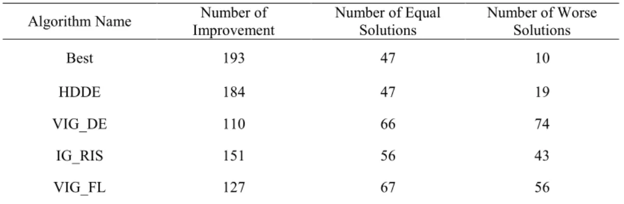
Table 6. Comparison of GVNS with competing algorithms ... 43

(11)

INDEX OF SYMBOLS AND ABBREVIATIONS

Symbols Explanations

machine no-idle permutation flowshop problem with makespan minimization

, jobs, total number of jobs

, machines, total number of machines

processing time of job j on machine

m

starting time of processing jobs on machine k

, job permutation, jth job of

permutation

( ) completion time of on machine k

makespan

population size

mutation scale factor, crossover

probability Abbreviations

PFSP permutation flowshop problem

NIPFS no-idle permutation flowshop

(12)

IG Iterated Greedy

VNS Variable Neighborhood Search

GVNS Global Variable Neighborhood Search

TFT total flow time

IG_LS iterated greedy with local search

VIG_FL variable iterated greedy by Framinan and Leisten

DE differential evolution

DDE discrete differential evolution

HDDE hibrit discrete differential evolution

VIG_DE variable iterated greedy with differential evolution

VND variable neighborhood descent

ILS iterated local search

RIS referenced insertion

(13)

CHAPTER 1 INTRODUCTION

A flowshop is a commonly used production system in manufacturing industries. Generally, in manufacturing environments, the jobs should go through different processes till the end items are obtained. If the route of each job is different, then this environment is referred as jobshop. The production environment with all jobs have the same route is called flowshop. Scheduling of a flowshop has an essential role in competitive environments; therefore this problem has been one of the most attractive subjects for researchers.

In a flowshop, there is more than one machine and each job must be processed on each of the machines. Each job has the same ordering of machines for its process sequence. Each job can be processed on one machine at a time, and each machine can process only one job at a time. For the permutation flowshop, the processing sequences of the jobs are the same on each machine. In other words, jobs have a permutation and therefore, once a permutation is fixed for all jobs on the first machine, this permutation is maintained for all other machines. If one job is at the position on machine 1, then this job will be at the position on all the machines.

In order to measure the performance of scheduling in a flowshop, there are several criteria such as, makespan and due-date based performance measures. Makespan criterion, without any doubt, the most widely used performance measure in the literature. The popularity of makespan criterion comes from the ease of implementation of this criterion to each kind of problem. On the other hand, in real life considerations, meeting customers’ requirements on-time is essential for several industries. For these problems which aim to satisfy promised due dates to customers, due-date based performance measures have been attracted interest from the researchers recently. There are many interesting and successful studies that are considering total tardiness criterion in literature as well.

In this thesis, a variant of permutation flowshop scheduling problem (PFSP), where no-idle times are allowed on machines, is considered. The no-idle constraint has an important role in scheduling environment, where expensive

(14)

machinery is employed. Idling machines in such environments is not cost-effective. Another situation that production environment desires to have no-idle times in schedule, is when high setup time or costs exist so that shutting down the machines after initial setup is not wanted. In no-idle permutation flowshop scheduling (NIPFS) problem, each machine must process each job without any interruption from the beginning of the first job to the completion of the last job. In order to meet this constraint, delays may occur in the processing of the first job on any machine. There are various examples of this problem in manufacturing industries. For instance, fiberglass processing has both costly and time consuming setups where the furnaces must be heated up to 2800ºF which takes three days. So furnace must stay on during the entire production to avoid long setup times but at the same time, since the cost of idling furnace is too high, the production must be scheduled considering no-idle restriction. (H. Saadani, A. Guinet, M. Moalla, 2003) presented a three-machine flowshop production of engine blocks in a foundry.

is a well-known notation of the m-machine NIPFS problem where the makespan is minimized. (Baptiste, P., & Lee, K. H., 1997) showed that is an NP-hard problem. Although it has a great importance in both theory and practical applications, it has not attracted much attention in the literature by the researchers. In (Adiri, I. and Pohoryles, D., 1982) an algorithm to solve optimally, is presented. The first time, problem is studied with the makespan criterion in (Vachajitpan, 1982). (Woollam, 1986) examined heuristic approaches for the general m-machine no-idle PFSP with the makespan criterion.

Recently, heuristic approaches have attracted increasing attention by many researchers. The solution quality of heuristic approaches started to get higher especially when the low computational effort is considered. A heuristic, based on the traveling salesman problem (TSP), for the the was represented in (Saadani, N. E. H., Guinet, A., and Moalla, M., 2005). (Kalczynski, P.J. and Kamburowski, J., 2007) presented an adaptation of the NEH heuristic for the NIPFS problem and also studied the interactions between the idle and no-wait flowshops. In (Ruiz, R. , Vallada, E. , Fernández-Martínez, C., 2009), an IG algorithm for the NIPFS problem with the makespan criterion was presented and examined the performance against the existing algorithms. (Tasgetiren M.F., Pan

(15)

Q., Suganthan P.N.,Oner A.) presented a discrete artificial bee colony algorithm to solve the no-idle permutation flowshop scheduling problem with the total tardiness criterion. (Kirlik G., Oguz C., 2012) applied a different algorithm to a different problem; the single machine scheduling problem to minimize the total weighted tardiness with the sequence dependent setup times by using general variable neighborhood search (GVNS) algorithm. This algorithm resulted very well for that NP-hard problem, therefore, inspiring from (Kirlik G., Oguz C., 2012), in this study, a GVNS algorithm is proposed to solve the NIPFS problem with makespan criterion and compared the results with some other algorithms to measure the performance.

This paper is organized as follows. In Chapter 2 NIPFS problem is defined. Details of metaheuristic algorithms are given in Chapter 3. Computational experiments that evaluate the performance of the solution methods are reported in Chapter 4. Finally, conclusion is given in Chapter 5.

(16)

CHAPTER 2 NO-IDLE PERMUTATION FLOWSHOP SCHEDULING

PROBLEM

No-idle permutation flowshop scheduling is required when the production environment desires to have no-idle times in production schedule because of the high costs or setup complexity of the system. In order to avoid the troubles in the production environment, the schedule must be done carefully while considering the all systems behavior.

There are jobs to be processed successively on machines with the same sequence on each machine. Associated with each job and machine , there is a processing time .

The assumptions for this problem are introduced;

 Each machine can perform at most one job at any given time;

 Each job can be processed on at most one machine at any given time;

 Processing sequences of jobs are same on each machine;

 There cannot be idle times between the start of processing the first job to the completion of processing the last job on any machine. While constructing the algorithm that will determine the production sequence of jobs, the time complexity of performance measures must be considered as well as problems’ objective, which is the makespan minimization for this problem. Both the reliability and the speed of the algorithm have an essential importance for real life problems. In real life problems, it is desirable to have a good quality solution in a short time period. In order to provide this, researchers have been studying on decreasing the time complexity of algorithms. (Ruiz, R. , Vallada, E. , Fernández-Martínez, C., 2009) proposed a formulation to calculate makespan of no-idle flowshop. In this formulation, first, when a given

machine can start processing with no needed idle time is calculated. Then by

using these values, the completion times are calculated straight forward, by adding processing times of jobs to the starting times for each machine, since the jobs are processed with no-idle time. Moreover, (Pan, Q-K. and Wang, L., 2008) also presented a formulation for the NIPFS problem with the makespan criterion.

(17)

This formulation consists of forward and backward pass calculation. These methods decrease the time complexity of calculating the completion times comparing to (Ruiz, R. , Vallada, E. , Fernández-Martínez, C., 2009) calculation method, which is a very desirable property especially in algorithmic studies. Less CPU time for calculation, provide opportunity to algorithm to apply more moves or to generate more generations that increases the chance to obtain more improved solutions.

In the formulation that (Ruiz, R. , Vallada, E. , Fernández-Martínez, C., 2009) used in their study, the necessity of the delay of the jobs, to ensure that jobs are processed without idle time, is considered and according to this feature, they proposed to first calculate the starting time of processing jobs on each machine which is denoted by where and denotes the machine. Then by adding the processing times to these starting times, they calculate the completion times. Let, a job permutation, be the sequence of jobs to be processed on each machine and the completion time of on machine be ( ). The formulations are given below;

{∑ ( ) ∑ ( ) }

(1)

After calculating the values, the completion time of each job can be calculated by adding the processing times of jobs on each machine;

(2) ( ) ( ) ( ) , (3) As a result, the completion time of jobs on the last machine gives the makespan;

. (4)

In order to come up with the complexity, the summations inside the max term in expression (1) have to be stored at each step. For example:

(18)

As mentioned before, (Pan, Q-K. and Wang, L., 2008) proposed another calculation method for NIPFS problem that consists of forward and backward passes which is explained in the following sections.

2.1 Forward Pass Calculation

Let the partial sequence of , represent the sequence of jobs from the first job to the job of sequence where . The minimum difference, between the completion of processing the last job of on machines and is denoted as and restricted by no-idle constraint. can be computed as shown below.

The completion time of last job, on last machine can be calculated as summation of value for all machines and the processing times of all previously processed jobs including itself;

∑ ∑ ( ) (8) Then, for any job , completion time on last machine can be computed by subtracting the processing time of the next job, from the completion time of

on machine ;

( ) ( ) ( ) (9) Makespan can also be defined as the maximum completion time of jobs on the last machine by using the no-idle constraint of this problem;

(10) And, the total flow time of the permutation , can be obtained as a summation of all completion times;

(20)

t M1 M2 M3 1 1 1 2 2 2 3 3 3 Machine

 

 max C

 



 n j1pj,1



3,1,2



E F _F



_₃E,2,3



Figure 4. Computation of

For the example instance for 3-job 3-machine problem that is taken from (Tasgetiren M.F., Pan Q., Suganthan P.N.,Oner A., In press), Figure 1 a to Figure 1 d, the forward calculation is illustrated with a permutation .

An example for forward pass calculation is represented below. Example

An example instance is given in Table 1 for 3-job 3-machine problem with permutation and with due date tightness factor of . According to the data given, the forward pass calculation is presented below, in detail.

Machines (k) Jobs (j) 1 2 3 4 1 3 2 3 3 2 2 3

Table 1. An example instance for forward and backward pass calculation

By using the equation (6), ( ) for the first job is computed as;

(21)

Equation (7) is used to calculate ( ) for the remaining jobs. For and ; For and ;

The completion time of the last job on last machine which gives also the makespan of the permutation is computed by using the equation (8);

∑

∑ ( )

For remaining jobs, completion time on last machine is computed by using equation (9);

The makespan can also be computed by using (10);

As mentioned before, the makespan calculation by using equation (8) and equation (10) results same since the problem has a no-idle constraint.

(22)

∑ ( )

2.2 Backward Pass Calculation

Let, the partial sequence of , represent the sequence of jobs from the _{job to the last job of sequence where . And let} be the lower bound for the minimum difference between the start of processing the first job of on machines and . Then;

E Figure 7. Computation of ( )

The completion time of the first job on last machine can be obtained as follows;

∑

(14)

Then, the completion time of any job on the last machine can be computed as;

( ) ( ) (15) The objective of no-idle permutation flowshop is to find the permutation which has a minimum makespan or total flow time in the set of all permutations ∏. The permutation can be obtained as;

or , ∏ (16) or , ∏ (17) t 1 2 3 1 1 1 2 2 2 3 3 3 Machine



1F,1,2



E



₁F,2,3



E _n_

 

j1pj,3

 

 max C Figure 8. Computation of

(24)

Fig. 2 a to Fig.2 d illustrate the backward pass calculation of makespan for a 3-job 3-machine problem.

By using the example instance that is given in Table 1, a detailed backward pass calculation is represented below.

Example

For the last job , is computed by using equation (12);

Equation (13) is used to calculate for the remaining jobs. For and ; For and ;

The completion time for the first job on the last machine , is obtained by equation (14);

∑

Using equation (15), all other remaining jobs’ completion time on last machine is computed;

(25)

As mentioned before, the makespan can also be computed by using (10);

And the total flow time can be calculated same as forward pass method by using equation (11).

As a result of this comparison study, the formulation of (Pan, Q-K. and Wang, L., 2008) is selected to use in this study.

(26)

CHAPTER 3 METAHEURISTIC ALGORITHMS

In the last years, a new kind of approximate algorithm started to be used by many researchers, which basically tries to combine basic heuristic methods in higher level frameworks aimed at efficiently and effectively exploring a search space. These methods are called metaheuristics.

Metaheuristic algorithms basically aim to provide nearly-optimal solutions by creating an initial solution and improving this solution iteratively. These algorithms help researchers to have qualified solutions for very complex problems (i.e. NP-Hard problems) which are commonly needed to be solved in real-life cases. There are several algorithms presented in literature; some of these algorithms uniquely developed for a specific problem, some of these are applicable for different types of problems. (Stützle, 1999) presented the definition for the term metaheuristic as follows;

“Metaheuristics are typically high-level strategies which guide an underlying, more problem pecific heuristic, to increase their performance. The main goal is to avoid the disadvantages of iterative improvement and, in particular, multiple descents by allowing the local search to escape from local optima. This is achieved by either allowing worsening moves or generating new starting solutions for the local search in a more “intelligent” way than just providing random initial solutions. Many of the methods can be interpreted as introducing a bias such that high quality solutions are produced quickly. This bias can be of various forms and can be cast as descent bias (based on the objective function), memory bias (based on previously made decisions) or experience bias (based on prior performance). Many of the metaheuristic approaches rely on probabilistic decisions made during the search. But, the main difference to pure random search is that in metaheuristic algorithms randomness is not used blindly but in an intelligent, biased form.”

In literature, for NIPFS problem, many researchers proposed different algorithms. In this thesis, the results obtained from four different algorithms that are proposed for the NIPFS problem, are compared with the proposed GVNS algorithm. These algorithms are;

An Iterated Greedy (IG_LS) algorithm for the NIPFS problem with the makespan criterion that is presented in (Ruiz, R. , Vallada, E. , Fernández-Martínez, C., 2009)

(27)

Variable Iterated Greedy (VIG_FL) algorithm, that is presented and implemented to solve the PFSP with the total tardiness criterion in (Framinan and Leisten, 2008)

The Hybrid Discrete Differential Evolution (HDDE) algorithm that is proposed by (Deng G and Gu X., 2012)

Variable Iterated Greedy algorithm with Differential Evolution (VIG_DE).

In this chapter these algorithms and the algorithm that is proposed; a GVNS algorithm with insert and swap operations in outer loop and in the inner loop (VND), IG algorithm and iterated local search (ILS) algorithm are explained.

3.1 Iterated Greedy (IG) Algorithm

Iterated Greedy algorithm is presented in (Ruiz R., Stützle T., 2007), based on a very simple principle and easy to implement as well as has successful applications in discrete/combinatorial optimization problem. It produces solutions with very good quality in a very short amount of time.

Algorithm starts with an initial solution that is generated either randomly or using heuristics, such as NEH heuristic that is explained in Section 3.1.1 . Then Destruction Construction Procedure is applied which is presented in Section 3.1.2 and repeated until some stopping criterion like a maximum number of iterations or a computation time limit is met. An optional local search phase can be added before the acceptance test for improving the re-constructed solution. For this study, Referenced Insertion Algorithm is used as a local search and explained in Section 3.1.3. . The pseudo code of the algorithm is given below;

//(optional) Local Search //Acceptance test { ( ) }

(28)

//Stopping criterion

Figure 9 Iterated Greedy Algorithm

3.1.1 The NEH Heuristic

NEH heuristic is proposed by (Nawaz, M., Enscore, Jr, E. E., and Ham, I., 1983) and has been recognized as the highest performing method for the permutation ﬂowshop scheduling problem. The NEH algorithm is based on scheduling jobs with high processing times, as early as possible, on all the machines. The NEH heuristic has three phases:

1. For each job , the total processing time on the machines are computed: ∑ ,

2. Jobs are sorted in descending order of . Let the resulting permutation be , then the first two jobs are selected and two possible permutations are generated and the one that results with the minimum makespan or total flowtime is selected.

3. Second phase is repeated until all jobs are sequenced. In order to generalize the procedure; in the _{step, the job} _{at position}_{is taken} and inserted into possible positions of the permutation of the jobs that are already scheduled. The best resulting permutation is selected.

The computational complexity of the NEH heuristic is , which consumes a very high level of CPU especially for larger instances. There are some speed-up methods that are introduced to reduce the complexity of NEH to . It is claimed that these speed-up methods are one of the key factors to the success of most algorithms especially the ones with the makespan criterion. Even though, in this study no speed-up method is used, the result of the proposed algorithm is way better than most of the algorithms from the literature.

3.1.2 Destruction and Construction Procedure

Destruction and Construction Procedure consists of two main steps; destruction step and construction step. In the destruction step, pre-determined

(29)

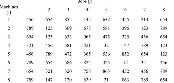
parameter many jobs are randomly chosen and removed from the current solution. Therefore, two partial solutions obtained; one consists of the removed jobs, in the order which they removed denoted as , the other one is the remaining part of the initial solution with size and denoted as . In the construction phase, a heuristic called NEH insertion is used. In this heuristic, basically all jobs in is inserted into each position in one by one, and finally the best permutation with the minimum makespan (or total tardiness) is selected. In a more detailed way; the first job of the is selected and removed from and inserted into all possible positions, thus many partial solutions obtained. By considering the performance criterion, the best solution is selected and kept. Next, the same procedure is applied for second job, third job and so on, until the is empty. Therefore, the size of becomes again. In order to be more descriptive, an example that is represented in (Ruiz R., Stützle T., 2007) is given below. Jobs (j) Machines (i) 1 2 3 4 5 6 7 8 1 456 654 852 145 632 425 214 654 2 789 123 369 678 581 396 123 789 3 654 123 632 965 475 325 456 654 4 321 456 581 421 32 147 789 123 5 456 789 472 365 536 852 654 123 6 789 654 586 824 325 12 321 456 7 654 321 320 758 863 452 456 789 8 789 147 120 639 21 863 789 654

Table 2. An example instance for Destruction and Construction Procedure

For the example instance given in Table 2, one iteration of the IG algorithm is applied. Let the given sequence given below be the initial solution that is obtained by using NEH algorithm with .

(30)

For the destruction phase, let the destruction size be, . Then, three jobs must be randomly chosen and removed from the current solution. Let these jobs be 5, 1 and 4, respectively.

7 3 4 1 8 2 5 6

Then, the removed job to be reinserted, and the partial sequence to be reconstructed becomes as follows, respectively;

5 1 4

7 3 8 2 6

In construction phase, each job in is reinserted in all possible positions in and the sequence with the best performance is selected. In the figures below, the best sequence after the reinsertion of each job is given.

After reinserting job 5, After reinserting job 1, After reinserting job 4,

The example shows that a new solution obtained by removing jobs 5, 1 and 4 and reinserting them, is which is a better solution than the inital solution given by the NEH heuristic ( ). This new solution is accepted by the acceptance criterion since it is better than the starting solution. Furthermore, this new sequence is known to be an optimal solution for this instance.

3.1.3 Referenced Insertion Algorithm

In the referenced insertion (RIS) procedure, as an initial step, a referenced permutation, , is selected which is the best solution found so far. Then, the first job of the is determined and the position of this job is found in the current permutation . This corresponding job is removed from and inserted into all possible positions of permutation . Next, second job of the is found in the permutation , removed and inserted into the positions of its own permutation. And the procedure goes on in this way, until all the jobs in the is processed. For example, let the referenced sequence be, and the current

7 3 8 5 2 6 7 3 8 5 2 1 6 7 3 8 5 2 1 6 4 1 2 1 3

(31)

solution be . The RIS procedure selects the first job of , which is job 4 and finds it in the current sequence. It removes job 4 from and inserts into all possible positions in . The objective function values of these newly generated permutations are compared to and if any insertion is better than , then the current solution is replaced by that permutation obtained by the insertion. Then the RIS procedure takes the second job of the referenced sequence which is job 2 and finds it in . Procedure removes job 2 from current solution , and inserts it into all possible positions of . This procedure is repeated until is empty.

The RIS procedure claims to have better solutions since the jobs are selected by referring to a good quality solution instead of a random choice. The pseudo code of this algorithm is represented below;

( )

Figure 10. Referenced Insertion Algorithm

In this study, an IG algorithm with RIS local search is applied to NIPFS problem. In addition to IG, another powerful algorithm, Iterated Local Search (ILS) algorithm is also applied to this problem. In the next section, ILS algorithm is explained in details.

(32)

3.1.4 Iterated Local Search Algorithm

Iterated local search (ILS) is first presented in (H.R. Lourenc, O. Martin, T. Stützle, 2002) and known as a simple and powerful stochastic local search method. According to (H.R. Lourenc, O. Martin, T. Stützle, 2002), “ILS is a

simple and generally applicable stochastic local search method that iteratively applies local search to perturbations of the current search point, leading to a randomized walk in the space of local optima”. The main idea of iterated local

search (ILS) algorithm is to apply local search repeatedly to initial solutions obtained by perturbations of a previously visited locally optimal solutions. The simplicity, ease of implementation and at the same time efficiency of this algorithm makes this algorithm eligible.

In (Thomas Stützle, 2006), the application of ILS to the quadratic assignment problem is represented. In this study, as a second algorithm of VND phase of the GVNS algorithm is inspired by this application of ILS.

In ILS algorithm, there are some procedures to be specified. These are;  How to generate initial solution (GenerateInitialSolution),  Perturbation type (Perturbation),

 Acceptance criterion (AcceptanceCriterion),  Which local search to use (LocalSearch).

(Thomas Stützle, 2006), used a random assignment of items to locations as the initial solution (GenerateInitialSolution). The phase Perturbation exchanges randomly chosen items, corresponding to a random move in the k-opt neighborhood. (Thomas Stützle, 2006) decided to determine value by using VNS. In order to decide which solution to choose, as AcceptanceCriterion,

Better(s,s’) function is used. By using this function, good solutions ( ) are determined as;

{

where represents the objective function value for solution . In

LocalSearch phase, an iterated descent algorithm with a first improvement

pivoting rule is used. The pseudo code of the ILS algorithm is given below, in Figure 17.

(33)

Figure 11. The general outline for an iterated local search

where indicates that also the search history may affect the and decisions.

3.2 Variable Iterated Greedy Algorithm

Variable IG algorithm (VIG_FL) is presented and implemented to solve the PFSP with the total tardiness criterion in (Framinan and Leisten, 2008). This algorithm is inspired from the idea of neighbourhood change of the VNS algorithm that is explained in Section 3.5 . In (Ruiz R., Stützle T., 2007) it is shown that destruction of 4 jobs is most adequate, so in their study, the destruction size is used as a constant parameter which equals to 4. In VIG_FL, the destruction size is developed as a variable and at the beginning it is fixed at . If the solution is not improved, the destruction size is incremented by until the maximum destruction size which is (where indicates the number of jobs). At any destruction size, if there is an improvement in the solution, destruction size is again fixed at and search starts all over again. The pseudo code of VIG_FL is given below;

( )

(34)

( )

Figure 12. Variable Iterated Greedy Algortihm of Framinan and Leisten

3.3 Variable Iterated Greedy Algorithm with Differential Evolution

Standard Differential Evolution (DE) algorithm is introduced by (Storn R, Price K., 1997) for continuous optimization problems. DE algorithm is a population-based algorithm and there are three different individual types; target, mutant and trial. At the beginning, population is consisting of “population size” ( ) many target individuals. Mutant individuals are generated by applying

mutation operation and trial individuals are generated by crossover operation and

then applies selection operator to determine the new target individuals for the next generation.

Let denote the th individual of target population at generation . denote mutant and denote trial individuals. Mutant and trial individuals are generated as follows;

(18)

{

(19)

where , , and are random integers that are different than each other and , and take values between . is a random number between [ ), is the mutation scale factor from [ ) and is the crossover probability from [ ]. is a random integer from [ ]. For creating a mutant individual in (18), three different individuals are randomly chosen from target population and the

(35)

difference of two of these individuals’ th elements is multiplied with mutation scale factor and added to third individual’s th element. So that, new mutant individual’s th element is obtained. In (19), with crossover probability the trial individual is taken from mutant population, otherwise it remains same as target individual.

By using these formulations, (18) and (19), trial population is generated for and . In selection phase, target population and trial population is compared and the one with better objective function value is selected. This phase is performed as;

{

(20)

where is the objective function value for individual . These iterations go on until pre-determined stopping criteria is satisfied.

A modified VIG algorithm is also applied to NIPFS problem to compare the performance of proposed algorithm. (Tasgetiren M.F., Pan Q., Suganthan P.N., Buyukdagli O., 2013) proposed an algorithm that the standard DE algorithm is modified and applied such that the probability to apply IG algorithm to the specific individual in the target population and the parameter of IG, destruction size is a variable. Thus, this algorithm is a variable iterated greedy algorithm guided by differential evolution denoted by VIG_DE.

Basically, VIG_DE algorithm optimizes the probability to apply IG to an individual ( ) and the destruction size ( ) that is used as a parameter of IG, by using DE. In the initial population, the permutation of the first individual is constructed by using NEH heuristic. All the remaining individuals in the target population are generated randomly and NEH heuristic is applied each of them to start the algorithm with relatively better individuals. The destruction size, , is determined randomly and uniformly between . After generating target population and for each individual of that population, IG algorithm is applied the individuals in target population without considering the probability that guides algorithm either IG is applied or not. Next, is determined as follows;

∑

(36)

A uniform random number is generated between [0,1), if this number is less than the probability , IG algorithm is applied to the trial individual with the destruction size . This calculation gives a high ratio which means higher probability to apply IG, when the objective function value is lower (for minimization problem) for that individual. This means after applying IG if the objective function value gets better, then the probability to apply IG gets higher value.

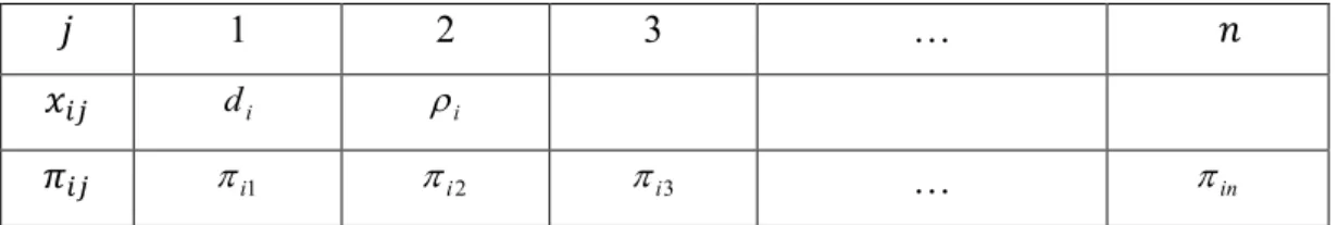
In order to avoid complexity, a unique multi-vector chromosome representation is used to keep all variables together in this problem. In Table 2, it can be observed that, the variables and appear in the first vector. corresponds to destruction size and to probability . The second vector contains the permutation that is assigned to each individual.

1 2 3 …

di i

i1 i2 i3 … in

Table 3. Multi-vector chromosome representation

In VIG_DE algorithm, mutant individuals are obtained by using formulation (18), for and , , and are randomly chosen integers by tournament selection with size of 2 that are different than each other and , and take values between .

For the crossover phase, an arithmetic crossover operator is applied to generate trial population.

(22)

where is a crossover probability from the range and . The higher value means, the higher effect of mutant individual comparing to target individual on the new trial individual. This arithmetic calculation may cause the individual to violate the search range. In order to fix this problem, following formulation is used;

(37)

where and , and is a uniform random number from . Since the first dimension is taken as a destruction size, this value should be an integer value. Therefore, destruction size is obtained by truncating such that; ⌈ ⌉. The second dimension is used as the probability to apply IG algorithm, . If a uniform random number is less than the probability , then the IG algorithm is applied and the fitness value of the generated trial individual is computed. In the selection phase, the survival of the fittest among all the trial and target individuals is considered as shown below;

{

(24)

Differential evolution part of the algorithm, that is explained above, is applied only the first vector of the solution representation which contains and . The pseudo code of the whole VIG_DE algorithm is given in Figure XXX.

Figure 13. Variable Iterated Greedy Algorithm with Differential Evolution

3.4 Hybrid Discrete Differential Evolution

The DE algorithm is proposed for continuous optimization problems where the individuals are represented by floating-point numbers, so in order to apply this algorithm to the problems where discrete job permutation is needed to be generated. (Tasgetiren, M. F., Pan, Q. -K., Liang, Y. -C., Suganthan, P.N., 2007a) proposed an algorithm for scheduling problems which is called Discrete

(38)

Differential Evolution (DDE) algorithm. Mutation and crossover operations are re-designed as job-permutation-based that is applicable for discrete cases.

The Hybrid DDE (HDDE) algorithm is the combination of DDE-based evolutionary searching technique and a problem specific local search. (Deng G and Gu X., 2012) inspired from (Tasgetiren M.F., Pan Q.K., Suganthan P.N., Liang Y.C., 2007b) study and applied their perturbed local search after the new population generated by using DDE which provides algorithm to start the new search with a qualified individuals. HDDE algorithm that (Deng G and Gu X., 2012) proposed is one of the metaheuristic algorithms that is compared with the algorithm presented in this study.

In this algorithm, the individuals are represented as job permutations; ( ). Different than standard DE that is explained in Section 3.3 , th individual of target population at generation is represented as

. Mutant and trial individuals are generated as follows;

{ ( )

(25)

{

(26)

where _{is a relatively better solution than current one, from generation} . operator is a random insert move in an individual , represents a crossover operator (partially mapped crossover) applied to and , is the insert mutation scale factor and is the crossover probability. is a random number between but different than and is a uniform random number between [ ). In (25), mutant individual is obtained as following; if is less than , insertion move is applied to a relatively better solution , otherwise to a random target individual different than th. Similarly, for the trial individual generation in (26), if is less than , partially mapped crossover is applied to mutant individual and the corresponding target value at the previous generation _{, otherwise mutant individual is directly taken.}

Selection phase of HDDE is performed same as in standard DE that is represented in (20) in Section 3.3 .

(39)

As a local search, in (Deng G and Gu X., 2012) perturbed local search is presented. This local search algorithm is a combination of destruction construction algorithm that is explained in Section 3.1.2 , referenced insertion algoritm that is presented in Section 3.1.3 and IterativeImprovement_Insertion that is represented in (Ruiz R., Stützle T., 2007). The outline of perturbed local search is shown below;

( ) ( ) { ( ) }

Figure 14. Perturbed Local Search

where is the best individual found by HDDE so far. For a given permutation , first destruction construction is applied, then insertion-based local search and lastly the acceptance criterion is checked.

The initial target population is generated randomly except two individuals of this population. One is generated by using NEH heuristic that is explained in Section 3.1.1, the other is generated by a variant of InsertionImprovement( ).

The pseudo code of HDDE algorithm is given below. This algorithm includes standard DE procedures, mutation, crossover and selection and as a local search perturbed local search.

(40)

Figure 15. Hybrid Discrete Differential Evolution

3.5 General Variable Neighbourhood Search

Variable neighborhood search (VNS) is a common approach to enhance the solution quality with systematic changes of neighborhood within a local search. It is proposed by (Mladenovic´, N., Hansen, P., 1997). The algorithm involves iterative exploration of larger and larger neighborhoods for a given local optima until there is an improvement, after which time the search is repeated. The basic steps of VNS algorithm can be summarized as given below:

Initially, a set of neighborhood structures, is selected where . Having a multi neighborhood structure makes VNS an effective algorithm since most local search heuristics use one structure, . Then the initial solution is generated either randomly or using heuristics, such as NEH heuristic. The stopping criteria can be selected as maximum CPU time allowed or maximum number of iterations. Then, following steps are repeated until the stopping criterion is met;

 Set ;

 Repeat the following steps until :

o Generate a point at random from _{neighborhood of} , (shaking)

o Apply local search method by considering as initial solution and obtain a local optimum denoted by . (local search)

o If this local optimum is better than , and continue search with current neighborhood structure meaning ; otherwise set .

There are some decisions to be made before using VNS algorithm. These are;  Number and types of neighborhoods to be used

 Order of their use in the search

 Strategy for changing the neighborhoods  Local search method

(41)

Shaking step of VNS algorithm provides randomness in search. If this step

is eliminated from algorithm, variable neighborhood descent (VND) algorithm is obtained. The steps of VND can be explained briefly, as follows;

 Set ;

 Repeat the following steps until : o Find the best

o If is better than , then set ; otherwise set .

An extended VNS algorithm called general variable neighborhood search (GVNS) that is proposed in (Hansen P., Mladenovic N., Urosevic D., 2006). It can be obtained by replacing the local search step of VNS with VND algorithm. In this study, a different version of the GVNS algorithm with insert and swap operations in outer loop and in the inner loop (VND), IG algorithm and iterated local search (ILS) algorithm is applied to NIPFS problem and compared to all other algorithms. Using an another algorithm in local search step of the VNS provides to have a more powerful algorithm.

The pseudo code of the GVNS algorithm we applied in this study is given below;

Figure 16. General Variable Neighborhood Search Algorithm

where, and operations. Shaking phase is composed of two different operations. The and operations applies only one insert and one swap move, respectively, to shake the permutation. The sequence of these operations has an

(42)

important role in search. In literature many study shows that putting insert operation before swap results better than the converse version. After shaking phase is applied, as a local search, and is explained below;

Figure 17. Variable Neighborhood Descent

where which is explained in Section 3.1 but with some differences. These differences will be shown in pseudo code given below.

, that will be explained briefly in Section 3.1.4 .

In phase, IG algorithm is applied until there is no improvement. After the neighborhood structure is changed as ILS algorithm. ILS algorithm is also applied as long as there is improvement. Otherwise the search is stopped.

Figure 18. The first neighborhood structure of VND in GVNS

In this study, as mentioned before, ILS algorithm is used as a second neighborhood structure in VND phase. Using that much powerful algorithm as a neighborhood structure instead of more basic ones, increase this phase’s ability to

(43)

reach better solutions. According to the No-Free Lunch (NFL) theorem that is proposed in (Wolpert D. H. and Macready W. G., 1997); “For any algorithm, any elevated performance over one class of problems is offset by performance over another class”. Meaning that, any algorithms performance may differ from problem to problem. So applying two different algorithms to a specific problem and changing the neighborhood while there is no improvement may increase the chance to get better solution. At some point, one of the algorithms may stuck and perform worse, when the neighborhood is changed, the other algorithm may perform very well.

Figure 19. The second neighborhood structure of VND in GVNS

where has a variable input that is called perturbation size and selected randomly between as applied and shown in (Pan, Q-K. and Wang, L., 2008) study that these interval results better than other. The perturbation is applied to permutation , that is obtained from the first neighborhood structure of VND. Perturbation strength many inserts are made in this step. Then, the local search RIS, that is explained in Section 3.1.3, is applied to newly generated permutation until there is no improvement.

(44)

CHAPTER 4 COMPUTATIONAL RESULTS

In this thesis, different algorithms that are proposed to solve no-idle permutation flow shop scheduling problem is compared with a newly modified GVNS algorithm, as mentioned in previous chapters. In Chapter 3, some metaheuristics that are applied to NIPFS problem from the literature are explained. Then, the computational results of these algorithms are compared with the GVNS algorithm.

In order to test the performance of these algorithms, the benchmark suite presented in the personal website of Ruiz García, Rubén1 is used. This benchmark is designed for NIPFS problem with makespan criterion specifically, with the number of jobs and the number of machines . There are 50 combinations with different sizes and each combination has 5 different instances. Thus, there are 250 instances in total. 5 runs were carried out for each instance for each algorithm. All results are compared with the best-known solutions presented in the website of Ruiz García, Rubén1

.

In order to compare these results, an average relative percentage deviation is calculated for each combination by using the following equation;

∑

( )_⁄

(26)

where is the objective function value that is obtained in run of each algorithm, is the best-known solution presented in the website of Ruiz García, Rubén1 and is the number of runs. The stopping criterion is selected as a maximum run time of each algorithm which is defined as milliseconds where the value of can be taken as, or depending on the comparison case. In the comparison tables, denotes that the algorithm was run for .

The proposed algorithms are coded in C++ and run on an Intel Core 2 Quad 2.66 GHz PC with 3.5 GB memory. The parameters of DE, the crossover

(45)

probability and mutation scale factor are taken as and , respectively. These high ratios provide algorithms to enhance the search space and to increase the diversification of solutions. The population size is taken as . For the Destruction and Construction procedure, the destruction size is fixed at .

The results of HDDE algorithm are taken directly from (Deng G and Gu X., 2012) study. They implemented the proposed algorithm HDDE to NIPFS problem with termination criterion of milliseconds where . There are a few differences in properties of their computer and the computer that is used in this study. These differences may cause an unfair comparison, therefore, in order to avoid this inequality, the algorithms other than HDDE were run with termination criterion milliseconds where . In other words, all other algorithms were run for half of the CPU time that HDDE algorithm was run for. The computational results are given in Table 4.

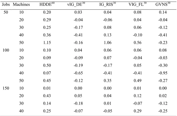
From Table 4, it can be observed that the proposed algorithm, GVNS, has better average relative percentage deviations than the other algorithms that applied to NIPFS problem. The GVNS algorithm was able to further improve the Best results to -0.213 which indicates that this algorithm is superior than the other four algorithms.

Table 4. Average relative percentage deviation of the algorithms

Jobs Machines HDDE60 vIG_DE30 IG_RIS30 VIG_FL30 GVNS30

50 10 0.20 0.03 0.04 0.08 0.14 20 0.29 -0.04 -0.06 0.04 -0.04 30 0.25 -0.17 0.08 0.06 -0.12 40 0.36 -0.41 0.13 -0.10 -0.41 50 1.15 -0.16 1.06 0.56 -0.23 100 10 0.10 0.04 0.06 0.06 0.08 20 0.09 -0.09 0.07 -0.04 -0.03 30 0.50 -0.19 -0.17 0.05 -0.30 40 0.07 -0.65 -0.41 -0.41 -0.95 50 0.45 -0.12 0.35 0.49 -0.27 150 10 0.01 0.00 0.00 0.01 0.00 20 0.43 0.05 0.04 0.12 0.02 30 0.14 -0.18 0.01 -0.07 -0.12 40 0.25 -0.07 -0.05 0.29 -0.25

(46)

Jobs Machines HDDE60 _{vIG_DE}30 _{IG_RIS}30 _{VIG_FL}30 _GVNS30 50 0.17 -0.85 -0.46 -0.57 -0.97 200 10 0.03 0.00 0.00 0.00 -0.00 20 0.04 -0.07 0.00 -0.01 -0.05 30 0.01 -0.31 -0.17 -0.20 -0.33 40 0.10 -0.26 -0.29 -0.26 -0.61 50 0.45 -0.40 -0.22 -0.17 -0.53 250 10 0.00 -0.01 0.00 0.00 -0.01 20 0.13 -0.03 0.05 0.02 -0.01 30 0.00 -0.14 -0.06 -0.12 -0.28 40 0.31 0.02 0.04 0.11 -0.14 50 0.06 -0.60 -0.77 -0.49 -1.09 300 10 0.00 0.00 0.00 0.00 0.00 20 0.12 0.00 -0.03 -0.03 -0.05 30 0.30 0.02 0.00 -0.06 -0.05 40 0.15 -0.34 -0.04 -0.17 -0.32 50 0.10 -0.23 -0.27 -0.15 -0.54 350 10 0.02 0.00 0.02 0.00 0.01 20 0.05 -0.01 0.02 -0.01 0.00 30 0.11 -0.05 -0.01 -0.08 -0.14 40 0.31 0.08 0.02 0.01 -0.17 50 0.18 -0.44 -0.40 -0.38 -0.72 400 10 0.01 0.00 0.00 0.00 -0.00 20 0.14 0.04 0.06 -0.01 0.00 30 0.23 0.11 0.05 -0.01 -0.02 40 0.20 -0.04 -0.09 -0.15 -0.16 50 0.08 -0.25 -0.28 -0.33 -0.49 450 10 0.02 0.00 0.00 0.00 0.01 20 0.12 0.00 0.04 0.00 0.04 30 0.08 -0.03 -0.09 -0.12 -0.16 40 0.01 -0.09 -0.02 -0.23 -0.23 50 0.21 -0.07 -0.27 -0.43 -0.53 500 10 0.01 0.00 0.01 0.00 0.00 20 0.04 -0.04 0.00 -0.04 -0.04 30 0.13 0.08 0.04 0.00 -0.05 40 0.13 0.10 -0.04 -0.04 -0.17 50 0.17 -0.03 -0.08 -0.23 -0.38 Overall Avg 0.16 -0.12 -0.04 -0.06 -0.213

(47)

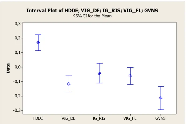
In order to determine if the average relative percentage deviations of algorithms are statistically significant, an interval plot is given in Figure 20. Vertical lines with horizontal lines at their end points represent the 95% confidence interval for the mean and the symbol at the middle indicates the mean of each algorithm’s relative percentage deviations. As can be observed from the interval plot, 95% confidence interval for the mean of GVNS algorithm is obviously does not coincide with the others which means that the means are statistically significant. In addition the mean of GVNS is significantly lower than the others.

Figure 20. Interval plot of algoritms compared

In Table 5, the best makespan values obtained by applying the compared algorithms to the benchmark suits are presented. The first three columns represent the number of jobs, number of machines and the instance number of the problem solved in that row, respectively. The column “Best” represents the best-known solutions presented in the website of Ruiz García, Rubén. The values in column HDDE60 are directly taken from (Deng G and Gu X., 2012), the remaining results obtained by applying these algorithms to the problem. For each row, meaning an instance, the minimum result is represented in bold font.

D a ta GVNS VIG_FL IG_RIS VIG_DE HDDE 0,3 0,2 0,1 0,0 -0,1 -0,2 -0,3

Interval Plot of HDDE; VIG_DE; IG_RIS; VIG_FL; GVNS

(48)

Table 5. Makespan values obtained by the algorithms

Jobs Machines Instances Best HDDE60_{VIG_DE}60_{IG_RIS}60_{VIG_FL}60_GVNS60

50 10 1 4127 4127 4127 4127 4127 4127 2 4283 4283 4283 4283 4283 4283 3 3262 3263 3262 3262 3262 3267 4 3219 3216 3216 3219 3219 3219 5 3470 3470 3470 3471 3471 3470 20 1 5647 5647 5647 5647 5647 5646 2 5834 5820 5818 5820 5820 5814 3 5794 5793 5793 5793 5793 5793 4 5803 5798 5799 5798 5795 5798 5 4907 4881 4884 4900 4897 4874 30 1 7243 7256 7223 7239 7239 7242 2 7381 7351 7351 7331 7330 7334 3 6902 6844 6857 6900 6885 6850 4 7624 7579 7579 7580 7580 7585 5 7340 7338 7333 7366 7366 7337 40 1 9264 9227 9168 9167 9130 9171 2 10164 10116 10137 10121 10117 10134 3 9896 9791 9782 9854 9836 9822 4 9575 9607 9523 9550 9533 9495 5 9082 8967 8968 8960 8957 8904 50 1 11652 11717 11604 11753 11753 11584 2 10946 10980 10893 10942 10942 10857 3 10960 10960 10885 10955 10935 10873 4 10026 10044 9967 10030 10030 9890 5 11380 11349 11316 11365 11348 11359 100 10 1 6575 6570 6570 6575 6575 6575 2 5798 5802 5803 5808 5802 5802 3 6533 6533 6533 6533 6533 6533 4 6161 6171 6158 6158 6158 6158 5 6654 6654 6654 6654 6654 6654 20 1 8611 8606 8606 8606 8606 8606 2 8223 8218 8224 8241 8241 8235 3 9057 9057 9043 9055 9043 9043 4 9031 9029 8972 8973 8970 8970 5 9126 9125 9109 9109 9109 9109 30 1 11249 11228 11210 11210 11202 11202 2 10989 10943 10938 10938 10938 10943 3 10666 10674 10571 10555 10555 10549

(49)

Jobs Machines Instances Best HDDE60 VIG_DE60 IG_RIS60 VIG_FL60 GVNS60 4 11175 11137 11103 11097 11097 11097 5 11030 11065 10983 10996 10985 10986 40 1 12806 12721 12606 12640 12640 12608 2 13306 13295 13117 13206 13202 13162 3 12654 12574 12488 12528 12504 12411 4 12044 11934 11781 11857 11829 11778 5 12934 12911 12920 12919 12919 12902 50 1 16111 16035 16019 16057 16050 15998 2 15019 14800 14787 14989 14916 14853 3 17755 17798 17585 17686 17650 17571 4 16672 16703 16684 16692 16667 16626 5 14827 14948 14802 14920 14854 14746 150 10 1 10404 10404 10404 10404 10404 10404 2 8824 8824 8824 8826 8824 8826 3 9180 9180 9180 9180 9181 9180 4 10032 10032 10032 10032 10032 10032 5 9870 9870 9866 9870 9870 9870 20 1 10768 10823 10758 10800 10790 10771 2 11718 11725 11699 11704 11699 11699 3 12063 12058 12046 12063 12060 12046 4 10965 11001 10936 10933 10933 10903 5 13210 13210 13210 13210 13210 13210 30 1 15569 15548 15505 15500 15500 15482 2 13747 13719 13667 13699 13667 13667 3 14688 14688 14651 14673 14651 14650 4 14627 14574 14549 14549 14549 14549 5 15257 15259 15265 15277 15277 15276 40 1 16217 16114 16025 16135 16120 15935 2 18235 18238 18122 18218 18173 18075 3 16416 16434 16356 16419 16381 16375 4 14658 14647 14648 14651 14640 14555 5 17298 17260 17246 17288 17244 17234 50 1 20625 20388 20364 20371 20367 20298 2 19512 19389 19121 19247 19227 19173 3 19702 19655 19447 19476 19358 19419 4 20355 20166 20139 20237 20224 20143 5 19611 19342 19308 19429 19418 19241 200 10 1 12155 12155 12155 12155 12155 12155

Metaheuristics for the no-idle permutation flowshop scheduling problem

METAHEURISTICS FOR THE NO-IDLE

PERMUTATION FLOWSHOP SCHEDULING

PROBLEM

Özge BÜYÜKDAĞLI

METAHEURISTICS FOR THE NO-IDLE

PERMUTATION FLOWSHOP SCHEDULING

PROBLEM

Özge BÜYÜKDAĞLI

TEXT OF OATH

ÖZET

BEKLEME ZAMANSIZ PERMÜTASYON AKIŞ TİPİ

ÇİZELGELEME PROBLEMİ İÇİN SEZGİSEL YÖNTEMLER

ABSTRACT

METAHEURISTICS FOR THE NO-IDLE PERMUTATION

FLOWSHOP SCHEDULING PROBLEM

ACKNOWLEDGEMENTS

TABLE OF CONTENTS

LIST OF FIGURES

LIST OF TABLES

INDEX OF SYMBOLS AND ABBREVIATIONS

CHAPTER 1

INTRODUCTION

CHAPTER 2

NO-IDLE PERMUTATION FLOWSHOP SCHEDULING

PROBLEM

























 

 























 

















 

 

CHAPTER 3

METAHEURISTIC ALGORITHMS

CHAPTER 4

COMPUTATIONAL RESULTS

.