KADIR HAS UNIVERSITY
GRADUATE SCHOOL OF SCIENCE AND ENGINEERING
LOCATION ESTIMATION OF BASE STATION OF MOBILE
PHONES USING ARTIFICIAL NEURAL NETWORKS
RAMAZAN CENGİZ
January, 2016
Ram az an C en giz M S T he sis 20 16
LOCATION ESTIMATION OF BASE STATION OF MOBILE
PHONES USING ARTIFICIAL NEURAL NETWORKS
RAMAZAN CENGİZ
B.S., Computer Engineering, Kadir Has University, 2012
Submitted to the Graduate School of Kadir Has University In partial fulfillment of the requirements for the degree of
Master of Science in
Computer Engineering
KADIR HAS UNIVERSITY January, 2016
iii
LOCATION ESTIMATION OF BASE STATION OF MOBILE
PHONES USING ARTIFICIAL NEURAL NETWORKS
Abstract
Finding the location of the base station of mobile phones is a problem. There are different approaches and methods for finding location in the literature. A solution to this problem is using “supervised learning” method. Recently, supervised learning technology is used in solving problems. For example, computer is trained and fed by necessary data. This data includes input and ideal targets. After computer is trained properly, it can make estimations of new data and give reasonable results. For the base station estimation program, mobile phone data(as input) of mobile phones and base station locations(as targets) are given to software. Software can estimate base location with input data, after training software
Matlab is a good program for supervised learning methods and artificial neural networks. For finding the optimal neural network topology and optimal training methods, Matlab is used in this project. Experiments are made with different data,different neural networks and different training methods. Results and outputs are observed. After finding best neural network topology, experiments are made with real data. Raw data are collected from mobile phones and after converting it into useful numbers and after normalizing these numbers, performance of the program is evaluated. Finally, this solution is implemented in Java platform. In this thesis, we present base location estimation program. This program takes as input a training data and test data. It uses training data to estimate the output of the test data. As output it creates a report that shows the estimated base station location.
v
MOBİL CİHAZLARIN BAZ İSTASYONLARININ YERİNİ SİNİR AĞLARI
KULLANARAK BULMA
Özet
Mobil cihazların sinyal aldığı baz istasyonlarının yerini bulma bir problemdir.Literatürde yer bulma için çeşitli yaklaşımlar ve yöntemler vardır. Bu probleme yönelik bir çözüm de”gözetimli öğrenimdir”. Günümüzde “gözetimli öğrenim” birçok problemin çözümünde kullanılır. Örneğin,bilgisayar ilgili veri ile eğitilir. Bu veri giriş verisive hedef verisini içerir. Bilgisayar bu veri ile eğitilmesinin ardından bir dahaki sefere yeni giriş verisi geldiğinde mantıklı çıktılar(sonuçlar) verebilir. Baz istasyonu yeri tahmin programı için giriş verisi mobil kullanıcıdan alınan giriş verisi ve hedef verisi(baz istasyonları yeri) programa verilir. Eğitim sonrasında yeni gelen giriş verisi bilgisayara verildiğinde ,bilgisayar baz istasyonu lokasyonu tahmini yapabilir.
Bu tezde, Matlab uygulamasından faydalanılmıştır. Matlab gözetimli öğrenimin yapay sinir ağları üzerinde uygulanması için iyi bir programdır. En iyi yapay sinir ağları topolojisini bulmak, en iyi eğitim metodunu bulmak için bu projede Matlab kullanılmıştır. Farklı verilerle, farklı yapay ağlarla ve farklı eğitim metodlarıyla deneyler yapılmıştır. En iyi yapay ağ teknolojisi bulunduktan sonra yapay veriden gerçek verilerle deney yapılmaya geçilmiştir. Cep telefonlarından ham veri toplanmıştır. Bu veri gereksiz bilgilerden ayıklandıktan sonra, sadeleştirilerek ve özeti alınarak anlamlı veri haline getirilmiştir. Sonrasında bu veri normalize edilerek programın çalıştırabileceği hale ve kullanıcıya kolaylık sağlar hale getirilmiştir. Sonrasında bu programın performansı deneylerle ölçülmüştür. En sonunda program Java platformunda implement edilmiştir.
vi
Bu tezde baz istasyonu yeri tespit etme programı anlatılmıştır. Bu program girdi olarak eğitim ve test datası alır. Bu program eğitim verisini kullanır ve kendisine verilen test verisinin çıktılarını buna göre tahmin eder. Çıktı olarak baz istasyonu yerlerini gösteren bir rapor verir.
vii
Acknowledgements
I would like to express my deep-felt gratitude to my advisor, Assistant Professor Selçuk Öğrenci of the Electronic Engineering Department at Kadir Has University. This thesis would not have been possible without his valuable guidance, constant motivation and constructive suggestions. He always gave me his time and support led me with constructive suggestions. I wish all students would benefit from his experience and ability.
Besides, I would like to thank Assistant Professor Taner Arsan of the Computer Engineering Department at Kadir Has University, for all supports they provided me throughout my all academic and graduate career.
I thank to my dear friend İlktan Ar and my all other friends who supported me during the thesis. And I thank Aykut Çayır who made the data collection mobile program.
Lastly, I thank to my family for their supports and understanding on me in completing this project. Without any of them mentioned above, I would face many difficulties while doing this thesis.
viii
Table of Contents
Abstract i Özet iii Acknowledgements v Table of Contents viList of Tables viii
List of Figures ix
List of Abbreviations xi
1 Introduction 1
2 Overview of Geolocation methods 5
2.1 Location accuracy methods... 5 2.2 Geolocation implementations... 8 3 Overview of Neural Networks and Training methods 15
4 Data collection 26
5 Algorithms and Source Code 39
6 Tests and Results 63
7 Conclusion 82
References 83
Curriculum Vitae 85
ix
List of Tables
Table 3.1:Training algorithms comparison Table 3.2:Training algorithms' performances Table 6.1: Matlab test results sample1 Table 6.2: Matlab test results sample2 Table 6.3: Encog test results sample1 Table 6.4: Encog test results sample2 Table 6.5: Encog test results sample3 Table 6.6: Encog test results sample4 Table 6.7 Encog test results sample5
Table 6.8: Resilient Propagation Comparisons Table 6.9: Levenberg Marquard Comparisons
x
LIST OF FIGURES
Figure 2.1: Cell of origin Figure 2.2: Time of arrival
Figure 2.3: Time difference of arrival Figure 2.4: Angle of arrival
Figure 4.1 : Database queries of data Figure 4. 2:Raw data
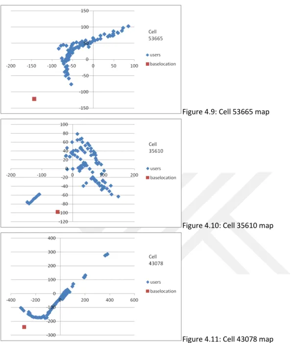
Figure 4. 3:Processed data Figure 4. 4:Final data Figure 4.5:Cell 6700 map Figure 4.6:Cell 29515 map Figure 4.7:Cell 40143 map Figure 4.8:Cell 37442 map Figure 4.9:Cell 53665 map Figure 4.10:Cell 35610 map Figure 4.11:Cell 43078 map
Figure 5.1:Flowchart of two outputs
Figure 5.2:Neural network topology for two outputs Figure 5.3:Flowchart of one output
Figure 5.4: Neural network topology for one outputs Figure 5.5: BrowseTrain Button
Figure 5.6: BrowseTest Button Figure 5.7: LoadNetwork Button Figure 5.8: TrainandTest Button Figure 5.9: LoadandTest Button
Figure 5.10: Levenberg-Marquard radio button Figure 5.11: Resilient Propagation radio button Figure 5.12: Hidden Layer Neuron InputText Figure 5.13: Output Neurons InputText
xi Figure 6.1: Base locations on map
Figure 6.2: Cell 6700 matlab estimation map Figure 6.3: Cell 11749 matlab estimation map Figure 6.4: Cell 29515 matlab estimation map Figure 6.5: Cell 32571 matlab estimation map Figure 6.6: Cell 29554 encog estimation map Figure 6.7:Cell 25625 encog estimation map
Figure 6.8: Cell 32430 encog estimation map Figure 6.9: Cell 35610 encog estimation map
Figure 6.10:Distance-Hidden Layer Comparisons in Resilient Propagation Figure 6.11:Distance-Hidden Layer Comparisons in Levenberg Marquard
LIST OF ABBREVIATIONS
Angle-of-Arrival: (AOA)
Cell identification: (Cell ID)
Global Positioning System: (GPS)
Round Trip Time :(RTT)
TDOA:(Time Difference of Arrival)
Time-of-arrival :(TOA)
1
Chapter 1
Introduction
The problem is to find the base station of mobile devices by using the most feasible methods. This problem, which we refer to as localization, is a challenging one, and yet extremely crucial for many applications of very large networks of devices[1]. There are some used methods in the literature.
A lot of related articles and presentations are read and know-how is acquired. Some of them are angulation, cell of identity, lateration and received signal strength methods. The first step is to investigate and find which method will help us more in the process. The most widely known, using the internal hardware of the cellphone, is satellite positioning using GPS but WiFi, Bluetooth, and augmented sensor networks can also be employed [2], [3], [4]. The cost, the easiness to implement and the performance of the methods are examined and comparisons are discussed.
The given input is the data of the mobile devices. The data gives the coordinates and received signal strength of the mobile devices. Boundary of the base station cell can be estimated by using this data . There are various methods for estimating the location of the base station. Firstly, location can be found by benefitting from the signal strength lines. Received signals can form a map in which various signal lines exist. Strong signal lines are closer to base station while weak signal lines are further to the base station. From this map the location of the base station can be approximated. In order to benefit from this data, data should be normalized. Then, it must be preprocessed. And after using the data, it should be post-processed. An improvement to the map model is to use artificial neural networks and learning methods. These methods help us predicting the values. This helps us make the
2
estimation process faster and more accurate. Moreover with these methods data can be visualized and controlled so good that data can be interpreted easier and better. These methods benefit from neural networks.
As an input that comes from the mobile phone is the longitude, latitude, cell identity and rscp values of the phone are taken and as output the longitude and latitude(location) of the base station is estimated. Neural networks are very helpful in achieving this aim. Once appropriate neural network is fed by appropriate data, if new data comes to trained artificial neural network, it can estimate the desired results. In this study artificial neural networks and supervised learning methods are used to find base location of mobile phones.
As the first step, a project planning is made. The steps that have to be taken are determined. Time planning is made. According to this plan, project progresses. Firstly, Matlab is used for the project with artificial data, then the project is realized by Java with real values. Raw data can't be used for the experiments on the neural networks. Some redundant data should be stripped from the main data. Furthermore data should be normalized. The normalization and cleansing of the data is one of the steps. By normalization,meaningful data is obtained.
Finding the best method for training is also a step.Firstly, the most suitable neural network has to be determined. Secondly, the most suitable training method has to be determined. The number of neurons in the input, output and hidden layers are determined. The optimum neuron numbers in the hidden layer will give best results. The most suitable transfer function in the hidden layers is important
Solution by Supervised Learning Method 1. Obtain data and data cleansing
3
For three different cell regions(dense urban, urban and rural) obtain data for the neighbour 10-20 cell information. After that, redundant and unnecessary data must be cleansed and finally, necessary and helpful data will be obtained
2. Data Preprocessing
Before we use the data in the program, data must be preprocessed. After the data is preprocessed, we can get better results easier.
• For every cell, record and base station data is normalized. There are 3 different methods.
• Normalize according to cell’s lower right corner. • Normalize based on cell’s geometrical middle point. • Normalize based on cell’s gravity center.
• Grouping : Cells form training, validation and test sets. 3. Realize algorithm by using Matlab
An algorithm must be made if we want to train data in Matlab. Matlab codes are used to realize the algorithm which trains data.
4
An algorithm must be made if we want to train data in Java. Encog libray and Java codes are used to realize the algorithm which trains data.
5.Training and Results
Final project stage is training. After enough trainings are made, results of the trainings will be discussed.
Dense urban training, urban training and rural training
Utilization of various artificial neural network topology. ( Neuron numbers in the hidden layer, hidden layer neuron numbers).
Objective: To find results for the test set using back-propagation training for data whose base station is known.
Input: Normalized longitude,latitude values.
5
Chapter 2
Literature Review
Overview of Geolocation methods
In this chapter, literature review about the geolocation methods will be explained. These methods are about locating a place on earth. They have already been used before. Each method has its own way to calculate the position of a place on earth. Each of them uses separate parameters to find location. After explaining theory of these methods,
implementations of these methods are discussed.
An Analysis of Base Station Location Accuracy
within Mobile-Cellular Networks
Received Signal Strength Indication (RSSI) measurements
RSSI beneftis from the received signal strength and its relation between the distance from the base stations(BS) to the mobile station. Due to the complex propagation mechanisms accuracy of this method is decreased.This problem, which we refer to as localization, is a challenging one, and yet extremely crucial for many applications of very large networks of devices.Radio propagation models [5] in various environments have been well researched and have traditionally focused on predicting the average received signal strength at a given distance from the transmitter (large scale propagation models), as well as the variability of the signal strength in close spatial proximity to a location (small scale or fading models).
Angle-of-Arrival (AOA)
It locates the mobile by using the angle-of-arrival(AOA) of a signal from many Base Stations(BSs) from the mobile. A line of bearing between the and mobile estimates the AOA distance. When multiple LOBs intersect, mobile position is estimated.
6
GPS (Global Positioning System)
The most accurate locationing metheod is GPS. It uses satellite signals and it provides accurate estimation.GPS solves the problem of localization in outdoor environmentsfor PC class nodes. But when signals are prevented, for example in indoors setting, Assisted GPS method needs hardware development.In addition new algorithms have greatly improved the accuracy and efficiency with which a cellphone can calculate its position [6], [7].
Time-of-arrival (TOA)
The fourth category determines mobile location by measuring the time-of-arrival (TOA) which provides the estimate of the distance between the BS and the mobile since electromagnetic waves propagate at the speed of light[8]. In this method, the mobile location is determined by measuring the time-of-arrival(TOA). The distance between the BS and the mobile is estimated by using electromagnetic wave propagation speed. When multiple TOAs intersect, mobile location is estimated. The most simple technic for GSM to measure the TOA is “ time advance”(TA). TA measures run-trip time between the BS and the mobile.
TDOA(Time Difference of Arrival)
TDOA(Time Difference of Arrival), is another technique based on propagation delay time. It calculates the differences in TOAs of a mobile signal at multiple pairs of BSs. Each TDOA forms a hyperbolic curve in which mobile may lie.
UL-TOA (Uplink TOA) and E-OTD (Enhanced ObservedTime Difference) are standard TDOA techniques for GSM networks. NLOS propagation and time synchronization between stations are potential disadvantages for propagation-time-based techniques.
Most feasible methods for location estimation of a cellphone within a mobile-cellular networks depends on the location of base stations(BSs) as known reference points for calculating the estimated position of the cellphone. The other techniques are WiFi,Bluetooth and augmented sensor networks. The accuracy of techniques depend on the technology,line-of-sight(LOS), and sensor network coverage. Assisted-GPS(A-GPS) uses mobile network information in combination with internal hardware of the cellphone. A-GPS uses network resources in the case
7
of poor signal reception. Location methods based primarily on mobile-cellular network information is popular.
Cell identification (Cell ID)
Cell identification (Cell ID) is the simplest location estimation method available, but also the least accurate[9]. A wedge shaped area, comprising roughly a third of the cell(for three sectored sites) is at best estimated. But if omnidirectional antennas in low-density single sector cells are used, entire circular area for sites can be included.
Round Trip Time (RTT)
Round Trip Time(RTT) is a measure of the distance. It measures the time taken by a radio signal to travel from the base station to cellphone and back. It reduces drastically the estimated location area compared to the Cell ID method for the same site.
Cell ID and RTT combine methods to provide an location estimation where these areas overlap
Location Accuracy
In addition to accuracy degrading, these challenges can also increase the cost of location estimation. These challenges are non-line-ofsight and multi-path propagation of radio waves, base station density(or lack of) and accuracy of base station locations.
The methods of location estimation consist of two groups. The first group doesn’t depend on base station location and aren’t affected by the accuracy with which these locations are known. These methods are A-GPS, probabilistic fingerprinting,bulk map-matching and centroid algoritm. The second group has methods that estimate location of the cellphone relative to the base station location and depend on the accuracy of network base station location. This group includes Cell-ID based methods,Cell ID and RTT,The time of arrival(TOA) and its enhancements.
8
Location Tracking Approaches(Implementations)
Location tracking and positioning systems are classified by the measurement techniques. These techniques are used to find the mobile device location(localization). Real Time Location Systems (RTLS) are grouped into four categories. They find the position on the basis of the following:
1. Cell of origin(nearest cell) 2. Distance(lateration) 3. Angle(angulation)
4. Location patterning(pattern recognition)
A RTLS designer can choose to implement one or more of the above techniques.
Cell of Origin
This method indicates the cell with which the mobile device is registered so it finds the position of the mobile device. Cell origin doesn’t need any complicated algorithm and thus its positioning performance is rapid. All cellular-based RF systems and cell-based WLANs can be easily and cost-effectively adapted to cell of origin positioning. This approach’s coarse granularity is a drawback. Some users who want more precise results also implement lateration,pattern recognition and angulation besides this technique for better results. Cell of origin figure is shown at Figure 2.1.
9 Figure 2.1: Cell of Origin
Distance-Based (Lateration) Techniques
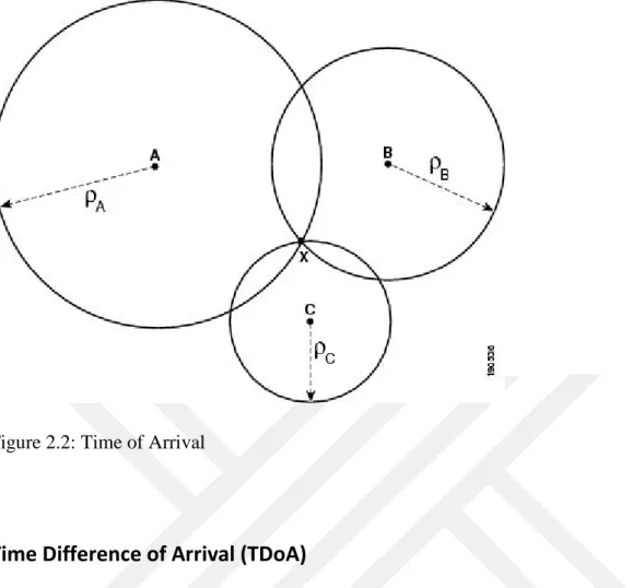
Time of Arrival(ToA) systems measure the arrival time of a signal transmitted from a mobile device to several receiving sensors. Signals travel with a known velocity(approximately the speed of the light.)The ToA requires that all receving sensors and the mobile device are synchronized with a precise time source. Distance can be thought as a radius of a circle area estimates the mobile location. Three sensors are implemented in ToA tri-lateration and this increases mobile location estimation accuracy. Three circular area of sensors give the estimated location . Large amount of multipath, interference, or noise creates error in ToA implemented positioning systems. The Global Positioning System (GPS) is a kind of ToA system. Timing is provided by atomic clocks precisely which is necessary in ToA systems. Figure 2.2 shows the mechanism.
10 Figure 2.2: Time of Arrival
Time Difference of Arrival (TDoA)
TDoA benefit from relative time measurement for each receiving sensor. Therefore TDoA doesn’t require a synchronized time source at the point of transmission as in the ToA systems.In TDoA systems only receivers need synchronization.
TDoA systems are implemented based on a mathematical concept known as hyperbolic lateration. In this method, at least three time-synchronized receiving sensors are needed. ToA and TDoA are similar. Both of these techniques proved to be successful for large-scale outdoor positioning systems. Figure 2.3 shows the hyperbols
11
Received Signal Strength (RSS)
Lateration can also be realized by using received signal strength(RSS) in place of time. RSS is calculated by either the mobile device or the receiving sensor. With this technique mobile device or receiving sensor measures the RSS. Transmitter output power, cable losses,antenna gains and path loss model allows to solve for the distance between two stations.
PL=PL1Meter+10log(d^n)+s
PL means path loss between the receiver and sender in dB
o • PL1Meter means the reference path loss in dB for the desired frequency when the receiver-to-transmitter distance is 1 meter.
• d means the distance between the transmitter and receiver in meters. • n means the path loss exponent for the environment.
• S shows the standart deviation related with the degree of shadow fading in dB.
• Path loss(PL) is the difference between the transmitted signal level and the received signal level. Path loss shows signal attenuation level present in the environment that is caused by free space propagation,reflection,diffraction and scattering.
RSS lateration techniques have a cost advantage because they don’t require any specialized hardware at the mobile device or network infrastructure locations
12
Angle-Based (Angulation) Techniques
Angle of Arrival (AoA)
The Angle of Arrival is also called Direction of Arrival. This method benefits from the angle of incidence at which receiving sensor takes the signal. Geometric relationships are used to determine location by using the intersection of two lines of bearing(LoBs) which is formed by a radial line to each receiving sensor. At least two receiving sensors are necessary but three or more receiving sensors increase accuracy.
Directional antennas deployed at the receiving sensors are adjusted to the signal with highest signal strength. The positioning of the antennas determine the LoBs and measure the angles of incidence.
Multiple tower sites obtain the AoA of the cellular user’s signal and use this info to perform tri-angulation. This info is converted to user location and latitude and longitude coordinates by the switching processors AoA works well with direct line of sight but its accuracy and precision decreases when confronted with signal reflections from objects.In practice this method requires expensive antenna arrays, which limit its feasibility despite its potential for high accuracy [9]. Figure 2.4 shows the angles.
13
Location Patterning (Pattern Recognition) Techniques
Location patterning basically samples and records radio signal behavior patterns in specific environments. A location patterning solution doesn’t require specialized hardware. Location patterning can be implemented fully in software therefore it reduces cost and complexity comparing to angulation or lateration systems.
Location patterning techniques require two fundamental conditions
• Each potential device location possesses a distinct and unique RF “signature”. • Each floor or subsection has unique signal propagation features.
Generally location patterning solution benefit from received signal strength(RSSI), pattern recognition may benefit from ToA,AoA or TDoA-based RF signatures as well. Patterning based positioning system consist of two phases:
• Calibration phase • Operation phase
During the calibration phase a database of RF signals are created. And during the operational phase the RF signature of the tracked device are matched with the database. The radio maps or calibration databases which is used by pattern recognition method are very specific to the areas used in their creation and it isn’t suitable for re-use. The radio maps or calibration databases which is used by pattern recognition method are very specific to the areas used in their creation and it isn’t suitable for re-use.
14
Okumura Model
The Okumura model is generally used in Urban Areas. It is a Radio propagation model. It is used for signal prediction. Its frequency range is 200Mhz-1900Mhz. Its distance range is 1km-100km. Antenna heights whose ranges 30m-300m is effective for base station. Okumura model has a 10-14db standard deviation. Its the deviation between the path loss model which is predicted by the model and the real measured path loss. Correlation factors related to terrain are calculated to improve the model accuracy.
Hata Model
The Hata model is an empirical formulation of data given by the Okumura. It is valid between 150-1500MHz. Hata model simplifies the path loss calculation since it has a closed form formula. Besides it doesn’t use empirical curves for the different parameters.
Hata model doesn’t use any specific path correlation factors. The Hata model gives more accurate results for distances d>1km. Hata models don’t capture indoor environments. Hata model is good at first generation cellular systems but it doesn’t model propagation well in new cellular systems with smaller sizes and high frequencies.
Okumura-Hata model (OH) [13] :
path_loss=158.3-13.82log(HBT )+(44.9-6.55log(HBT))log(d)
Where (HBT) is BS antenna height. ∆Hb is difference between BS antenna height and MS height (1.5m) and (d) is the BS-MS distance[14].
15
CHAPTER 3
Overview of Neural Networks
In this chapter, artificial neural networks and training will be explained. This is the theory part of the project. Various neural network types are discussed. Besides, various learning methods are discussed. Furthermore,various training methods are discussed. The details of training,test,train validation sets and improving results are discussed for an optimal neural network training.
Artificial Neural Networks
In computer science artificial neural networks are computational models that resemble animals’ biological central nervous system. Scientists who examined the central nervous systems inspired from them. Basically a class of statistical model which consist of set of adaptive weights, a learning algorithm with numerical parameters and which can approximate a function of their inputs can be called artificial neural network. Learning updates the weights.An activation function converts input to output. In artificial neural networks simple artificial nodes are called “neurons”,”units” or processing elements.The adaptive weights are used in training and prediction phases. They are connection strengths between neurons.
Learning paradigms
There are three major learning paradigms. 1-Supervised learning
2-Unsupervised learning 3-Reinforcement learning
16
Supervised learning
In supervised learning we have to infer the mapping from a given function, using the implied data.
As the name suggests, we have prior knowledge from the labeled data about the problem domain.
Basically we have to find a function from a given set of example pairs(x,y) to find f:X-> Y matching examples. Difference between our mapping and the data gives us the cost function. Some of application areas of supervised learning are pattern recognition(classification) and regression(function approximation). We use previous solutions as feedback in supervised learning.
.
Training:Basically, neural network’s function is to predict an output pattern when an input pattern is given. After a neural network is trained, it is able to recognize similarities when it is presented with a new input pattern. Therefore it results in a predicted output pattern.
Clustering:Clustering algorithm finds resemblances between patterns and puts similar patterns in its cluster.
Pattern recognition(Classification): When an input pattern is given, it is assigned to a class between some classes. This task is called pattern recognition.
Function approximation:Function approximation creates an estimate of the unknown function f() subject to noise.
Prediction/Dynamical Systems: When a time-sequenced data is given, some future values are estimated. This task is called prediction. Prediction is used widely in decision support systems and datawarehouses. The difference between prediction and function approximation is time factor. Prediction is a dynamical system and gives different results for the same input data but different system state(time).
Learning rate: The learning rate is value between 0 and 1. Weight adjusments size is controlled by it. Learning process speed is affected by it. In addition, precision rate of network is affected by it.
17
Difference between supervised learning and unsupervised learning: In supervised training, inputs and outputs are given. The network uses the inputs and compares its results with the desired outputs. Errors are calculated and according to this, the system adjusts the weights which control the network. This process is repeated many times and weights are changed. In unsupervised training the inputs are given to the network but outputs aren’t given to the network. The system itself decides the features which is needed to group the input data. This is called self-organization(adaption). For example learning process is usually unsupervised. Supervised Learning
In supervised learning a labeled training set is given. The class of inputs is provided and known. Unsupervised Learning
In unsupervised learning a set of patterns are given from n-dimensional space. But no/little information about their classification and evaluation is given
Tasks:
Vector Quantization: N-dimensional space S is divided into a small set of regions.(It is also useful in clustering pattern sets.)
Feature extraction: Feature extraction reduces the dimensionality of n-dimensional space S by removing unimportant features that don’t help clustering
Bias:Two different kind of parameters are modified during ANN training, the weights and the t values. “t” parameter is the amount of incoming pulses that is needed to activate a real neuron. This is not practical and it would be easier if only one parameter is modified. Bias neuron is invented to solve this problem.
18
Perceptron has many definitions but one of the simplest is this “A single layer network which produces a correct target vector when presented with the input vector.” [14]. This single layer does this training by changing the weights and biases of the network.
The training technique for the perceptrons is perceptron learning rule.
The perceptron contains a single layer. It is connected to R inputs with a set of weights. A perceptron is created with the newp function. net = newp(P,T)
The network includes zero weights and biases. If you want different weights and biases with values other than zero, you have to create them with command manually.
Set the two weights and the one bias to -1, 1, and 1 net.IW{1,1}= [-1 1]; net.b{1} = [1];
Now use init to reset the weights and bias to their original values: net = init(net);
A learning rule means a procedure to modify the weights and biases of a network. It is also called training. Learning rule is applied to network to do a specific task. If epochs is set to 1, train goes through the input vectors 1 time.
To set the parameter
time. net.trainParam.epochs = 1; net = train(net,p,t);
The outputs aren’t equal to the targets yet, so the network needs to be trained for more than one pass. More epochs are needed to find more accurate results. net.trainParam.epochs = 1000;
The default training function for networks created with newp is trainc. This fact can be verified by executing net.trainFcn (Youcan find this by executing net.trainFcn.)
19
Perceptron networks are generally trained with adapt function. Adapt function presents the input vectors to the network one at a time. After that corrections and adjusments are made to the network by the result of each input vector prestentation. In this way, it is guaranteed that any linearly separable problem is solved in finite steps training presentations.
Backpropagation
Back propagation is the most widely used algorithm for supervised learning with multi-layered feed-forward networks[15]. The basic idea of the back propagation learning algorithm [16] is the repeated application of the chain rule to compute the influence of each weight in the network with respect to an arbitrary error function E:
𝜕𝜕𝜕𝜕 𝜕𝜕𝑤𝑤𝑖𝑖𝑖𝑖 = 𝜕𝜕𝜕𝜕 𝜕𝜕𝑠𝑠𝑖𝑖 𝜕𝜕𝑠𝑠𝑖𝑖 𝜕𝜕𝑛𝑛𝑛𝑛𝑛𝑛𝑖𝑖 𝜕𝜕𝑛𝑛𝑛𝑛𝑛𝑛𝑖𝑖 𝜕𝜕𝑤𝑤𝑖𝑖𝑖𝑖
wij represents the weight from neuron j to neuron i, s; is the output, and neti represents the weighted sum of the inputs of neuron i.
Once the partial derivative for each weight is known, the aim of minimizing the error function is achieved by performing a simple gradient descent:
𝑤𝑤𝑖𝑖𝑖𝑖(𝑛𝑛 + 1) = 𝑤𝑤𝑖𝑖𝑖𝑖(𝑛𝑛) − 𝑛𝑛𝜕𝜕𝑤𝑤𝜕𝜕𝜕𝜕 𝑖𝑖𝑖𝑖(𝑛𝑛)
Backpropagation means backward propagation of errors. This is a training method used with gradient descent optimization method. The aim of the method is to calculate the gradient of a loss function according to the weights in the network. The gradient is used by the optimization method and optimization method uses it to update the weights.
Typically a network is given input and output. This way network learns . And if a new input is given it will produce output that is similar to the learnt correct output.
Neurons use a differentiable transfer function f to generate their output. Firstly, a feedforward network is created. . The third argument is an array containing the sizes of each hidden layer. In matlab net = newff(houseInputs,houseTargets,20); does this job.
20
While two-layer feed-forward networks can be trained and can learn almost any input-output relationship, feed-forward networks with more layers might learn complex relationships more quickly.
The weights and biases of the network are adjusted so that the error is minimized. This performance error function is net.performFcn in matlab. If any performance function isn’t specified, default function for it is mean square error(The average squared error between the network outputs a and the target outputs t) “mse” in matlab
During training the weights and biases of the network are iteratively adjusted to minimize the network performance function net.performFcn. The default performance function for feedforward networks is mean square error mse—the average squared error between the network outputs a and the target outputs t. net = newff(p,t,3,{},'traingd');
More optional arguments can be provided for the feedforward backpropagation method in the matlab. For instance, the fourth argument represents a cell array which contains the names of the transfer functions to be used in each layer. The fifth argument represents the name of the training function to be used. If only three arguments are supplied, the default transfer function of hidden layers is tansig and the default for the output layer is purelin. The default training function is trainlm.
net = newff(p,t,3,{},'trainrp');
net = newff(houseInputs,houseTargets,20); net = train(net,p,t);
Training,Validation,Test Datasets
In multilayer networks, firstly the data is divided into three subsets. The first subset is training subset. In training subset the gradient is computed and the network weights and biases are updated.
The second subset is the validation subset. The error on the validation set decreases during training phase with training set error. When network overfits the data,
21
validation set error starts to rise. At minimum validation set error the network weights and biases are saved.
The test set error is used for comparing different models. It is used when plotting the test set error during training.
In matlab four functions are used to divide data into training,validation and test sets. These are dividerand(the default),divideblock,divideint and divideind.
Training Set
The training dataset trains or builds a model. For instance, in a linear regression model the training dataset fits the linear regression model. Besides it is used to obtain regression coefficients. The training dataset finds the network weights in a neural network model.
Validation Set
After a model is built based on the training data, the accuracy of the model on unseen data is needed. Therefore data needs to be used on a dataset that wasn't used in the training process(This dataset has the actual value of the target variable) The small difference between the actual value and the predicted value of the target variable is the error in prediction. Some form of average error(for example MSE ) measures the overall accuracy.
The training data itself can't be used to compute the accuracy of model fit becuase model fit process ensures the training data is very accurate and therefore very optimistic estimates are obtained.So a part of the original data needs to be partitioned for realistic estimate with unseen data. This dataset is called validation dataset. After the model is fit on the traing dataset, its performance on the validation dataset is measured.
22
The validation dataset is used in fine-tuning of models. It can be used in various architectures. When finally a model is chosen after comparisons of architectures it may still give optimistic estimates because the final model is winner among the other models based on the validation dataset accuracy.
A portion of the original data that is neither used in training nor in the validation phase is set aside. This dataset is called test dataset.
The most realistic performance estimate of the model on completely unseen data is on the test data set.
Improving Results
After training the network, if it isn't accurate enough, the network can be initialized and it can be trained again. Each time a feedforward network is initialized, the network parameters change and it may produce different solutions.
This can be done in matlab by using init command. net = init(net);
net = train(net,houseInputs,houseTargets);
Secondly ,the hidden neuron number can be increased above 20. Larger neuron number gives the network more flexibility. Because the network can optimize more parameters. However too large hidden layers can optimize more parameters than data vectors which constrain these parameters.
Thirdly, a different training function can be used. For example Bayesian regularization training with trainbr sometimes produces better results than early stopping.
Eventually, using additional training data is good for better training. Feeding network with additional data produces a network that generalizes better to new data.[17]
23
The R value indicates the relationship between the outputs and targets. If R=1, this is the indication that outputs and targets have exact linear relationships. If R is close to zero this means there is no linear relationships between outputs and targets. After training the network the performance can be measured by the errors on the training, validation and test sets. However sometimes investigating the network response in more detail is needed. A good approach is a regression analysis between the network outputs and the corresponding targets. The regression method is designed to perform this analysis.
Training Algorithm
Problem Solution Class
Network Size
Levenberg-Marquardt
trainlm function approximation
medium
networks
24
BFGS Quasi-Newton
trainbfg function approximation
medium
networks
Resilient Backpropagation trainrp
pattern recognition
large
networks
Scaled Conjugate Gradient trainscg
pattern
recognition,function
approximation
large
networks
Conjugate Gradient with
Powell/Beale Restarts
traincgb
pattern
recognition,function
approximation
large
networks
Fletcher-Powell Conjugate
Gradient
traincgf
pattern
recognition,function
approximation
large
networks
Polak-Ribiére Conjugate
Gradient
traincgp
pattern
recognition,function
approximation
large
networks
One Step Secant
trainoss function approximation
large
networks
Variable Learning Rate
Backpropagation
traingdx
pattern
recognition,function
approximation
medium
networks
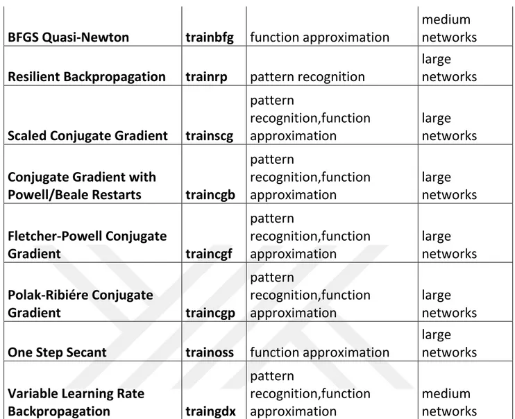
Table 3.1: Training algorithms comparison
Table 3.1 compares various training algorithms. Each training algorithm is good at solving its specific problem type or types. Besides, abbreviations of training algorithms are given. Furthermore, each training algorithm is good at specific network size. These attributes are listed and compared at the table.
25
Levenberg-Marquardt trainlm Very High High Cheap
Jacobian
matrix(easier than Hessian)
BFGS Quasi-Newton trainbfg High High Expensive
Second
derivative(Hessian matrix)
Resilient
Backpropagation trainrp Medium Medium weights change by derivative sign
Scaled Conjugate
Gradient trainscg High Low Cheap No line search
Conjugate Gradient with Powell/Beale
Restarts traincgb High Medium Medium
Less reset points for the direction of gradient
Fletcher-Powell
Conjugate Gradient traincgf High Low Medium conjugate search direction
Polak-Ribiére
Conjugate Gradient traincgp High Low Medium conjugate search direction
One Step Secant trainoss Medium Medium Medium
Compromise function between BFSG and
conjugate gradient
Variable Learning Rate
Backpropagation traingdx Medium Medium Cheap adaptive learning rate
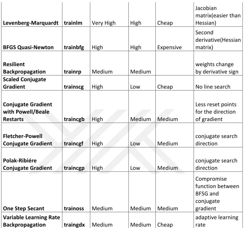
Table 3.2: Training algorithms performances
Table 3.2 lists and compares various training algorithms according to their performance, storage, computation and its special training method. Besides, abbreviations of training algorithms are given. Performance, storage and computation are important attributes in training. A training algorithm can be good in one attribute but it can be medium or poor in other attributes. User can decide a training algorithm according to his needs. “Special” column is specific method to related training algorithm.
26
CHAPTER 4
DATA COLLECTION
In the project, firstly raw data was studied. This raw data contained a lot of redundant information. Meaningful patterns had to be specified and an algorithm for this data had to be made. This algorithm aims to extract meaningful information from raw data. After that java parser code implements and realizes this solution. After that this meaningful data is analyzed in excel and access. Necessary normalizations are made and a training data is created.
Secondly, artificial data was studied. Artificial data is created by Dr. Selçuk Öğrenci. Real data is simulated and noise is added therefore artificial data is created. This simulated data was similar to real data. This data contains user location coordinates and rscp values. Rscp values indicate the signal strength between phone and base station. Experiments are made with this data on Matlab program and java encog library. Encog library is an open source machine learning library that contains training methods.
Finally, real data that comes from user mobile phones was studied. This data is collected by a mobile program. This program starts to collect user data as user presses “start” button. It finishes collecting data when the user presses “finish” button. A person has to go around certain locations to collect the user data at this location. This data was gathered by Dr. Selçuk Öğrenci. He wandered around certain locations with mobile phone and gathered user data. Later, programmer Ramazan Cengiz gathered user data by going around certain locations for additional data. This is real data and outputs are real values and locations. Experiments were made with this data on Matlab and Encog. This data contained data from 60-70 base stations. It contained tens of thousands of lines of data. Data was reduced to 20-30 base stations and data lines were reduced to hundreds of lines. This was realized by queries and analysis on excel and access. Finally, 21 training and 5 test sets were created.
27
Database code
In the project information for each cell was required. This information was concerned about cell normalization. This info has to show the estimated cell identity according to three normalization types(Gravity center coordinate,Geometric center coordinate, Minimum left point coordinate). In addition normalized coordinates(latitude,longitude values) has to be shown in the information document.
In the gravity center normalization gravity center of the cell is accepted as cell center and other points’ relative distance to center is calculated as its normalized value. In the geometric center normalization, geometric center of the cell is accepted as base station and other points’ relative distance to center is calculated as its normalized value. In the min normalization, minimum coordinates of the cell is accepted as base station and other points’ relative distance to center is calculated as its normalize value.
So, a cell id and all coordinate points belonging to this cell id needs to be collected. After these values are collected, gravity center of it is calculated,then geometric point of the cell and min,max points of the cell are calculated. After that process each cell id(base staion) has its own geometric center,gravity center and min,max points. Later on, the coordinates(longitude,latitude values) that belong to specific cells are normalized(the distance to center is calculated) so that they have new normalized values. This process makes the job easier in the training process.
28
1- Main data table named “tabela” is imported into Access database. This table contains “OMA specified longitude,latitude values” and their distances in km to (0,0)point in the map. X distances, Y distances and direct distances are held in this table.
2- By running query1 on table “tabela” ,a table named “QTABLO1” is formed. This table contains detailed data. Each cell’s longitude and latitude values are held in this table.
3- By running query2 on table “tabela” ,a table named “QTABLO2” is formed. This table contains summary main data. Each cell’s avg,min,max,geo values are held in this table
4- By running NormalizeQuery each longitude,latitude with its normalized values are obtained. This query includes a relationship between QTABLO1 and QTABLO2. By using inner join ” FROM QTABLO22 INNER JOIN QTABLO11 ON QTABLO22.UC=QTABLO11.UC;” Foreign key,primary key relationship is done.
29
NormalizeQuery
SELECT QTABLO22.UC AS QTABLO22_UC, QTABLO11.LATIY AS LATI, LATI-QTABLO22.avglat AS ["normlatavg"], LATI-QTABLO22.geolat AS ["normlatgeo"], LATI-QTABLO22.minlat AS ["normlatmin"], QTABLO22.minlat, QTABLO22.avglat, QTABLO22.geolat, QTABLO22.maxlat, QTABLO11.LONGIX AS LONGI, LONGI-QTABLO22.avglon AS ["normlonavg"], LONGI-QTABLO22.geolon AS ["normlongeo"], LONGI-QTABLO22.minlon AS ["normlntmin"], QTABLO22.minlon, QTABLO22.avglon, QTABLO22.geolon, QTABLO22.maxlon
FROM QTABLO22 INNER JOIN QTABLO11 ON QTABLO22.UC=QTABLO11.UC;
QUERY1(Detail table)
SELECT tabela.UC, tabela.LATIY, tabela.LONGIX, Count(tabela.UC) AS totalcell, Min(tabela.LATIY) AS minlat, Avg(tabela.LATIY) AS avglat, (minlat+maxlat)/2 AS geolat, Max(tabela.LATIY) AS maxlat, Min(tabela.LONGIX) AS minlon, Avg(tabela.LONGIX) AS avglon, ((minlon+maxlon)/2) AS geolon,Max(tabela.LONGIX) AS maxlon INTO QTABLO11 FROM tabela
WHERE (((tabela.UC) Is Not Null) AND ((tabela.LATITUDE) Is Not Null) AND ((tabela.LATITUDE) Is Not Null)) GROUP BY tabela.UC, tabela.LATIY, tabela.LONGIX;
QUERY2(Main table)
SELECT tabela.UC, Count(tabela.UC) AS totalcell, Min(tabela.LATIY) AS minlat, Round(Avg(tabela.LATIY),2) AS avglat, (minlat+maxlat)/2 AS geolat, Max(tabela.LATIY) AS maxlat, Min(tabela.LONGIX) AS minlon, Round(Avg(tabela.LONGIX),2) AS avglon, ((minlon+maxlon)/2) AS geolon,
Max(tabela.LONGIX) AS maxlon INTO QTABLO22 FROM tabela
30 Figure 4.1 : Database queries of data
31
MOBILE PHONE DATA COLLECT SOURCE CODE
public void run() //Create TelephonyManager Object
//GsmCellLocation gsmLoc = (GsmCellLocation) tm.getCellLocation();
//Log.d("ramco", gsmLoc.getCid() + ""); List<CellInfo> gcis = tm.getAllCellInfo();
File dir = Environment.getExternalStorageDirectory(); Calendar calendar = Calendar.getInstance();
SimpleDateFormat sdf = new SimpleDateFormat("dd-MM-yyyy"); if(gcis != null){
for(CellInfo ci : gcis){ String logStr = ""; if(ci instanceof CellInfoGsm){
//Log.d("GSM", "GSM_INFO"); //Log to GSM file
fileName = "gsmData_"+sdf.format(calendar.getTime())+".csv"; File logFile = new File(dir, fileName);
CellInfoGsm cgi = (CellInfoGsm)ci;
int rssi = cgi.getCellSignalStrength().getDbm(); long timestamp = cgi.getTimeStamp();
int lac = cgi.getCellIdentity().getLac(); int cid = cgi.getCellIdentity().getCid(); int mnc = cgi.getCellIdentity().getMnc(); int mcc = cgi.getCellIdentity().getMcc();
Above, mobile phone method code can be seen. Its "run" method is seen. Using the related library, cgi object is created. In cgi object, all necessary info about cell location is stored. These info is extracted and put into variables by using related methods such as getMNC,getCid,getMCC.
32 super.onCreate(savedInstanceState);
setContentView(R.layout.activity_main); //initialize & instantiate objects
state = false;
startBtn = (Button) findViewById(R.id.startBtn); stopBtn = (Button) findViewById(R.id.stopBtn); secText = (EditText) findViewById(R.id.sec);
locationManager = (LocationManager)getSystemService(LOCATION_SERVICE);
locationManager.requestLocationUpdates(LocationManager.GPS_PROVIDER, 0, 0, this); tm = (TelephonyManager)getSystemService(TELEPHONY_SERVICE);
startBtn.setOnClickListener(new OnClickListener() { @Override
public void onClick(View arg0) { int ms;
timer = new Timer();
if(secText.getText() == null || secText.getText().toString().equalsIgnoreCase(""))
ms = 3000;
Above, mobile phone code is seen. In this method GUI of the program is designed. GUI items, buttons and texts are assigned to program variables. Besides a timer object is created to specify the data collection time.
33
Raw Data
Figure 4.2: Raw data
This raw data is unprocessed data that is collected by the mobile phone. It is shown at figure 4.2.This data needs to be adjusted in order to be used by the program. Redundant data should be eliminated. Besides, necessary base locations need to be added for training. And
34
Processed Data
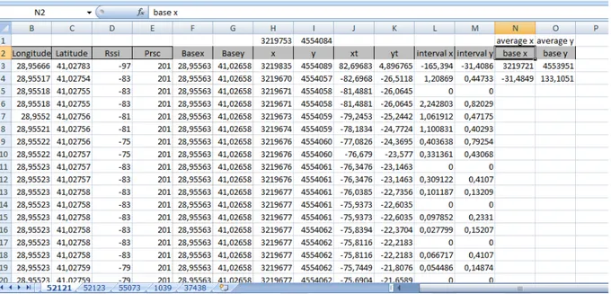
Figure 4.3: Processed data
This data is intermediate processed data. It is shown at figure 4.3. Average user x and average user y locations need to be found. According to these average values, normalization is made. This normalized values are small and more suitable for training. In addition, base x and base y locations need to be found. This is necessary for supervised learning and training data.
Interval x and interval y helps us to eliminate redundant and repeated data. 0 means the distance values are the same and redundant and isn't needed for training.
35
Final Train Data
Figure 4.4: Final Train Data
This is final train data. Only useful data is stored in the file. It is shown at figure 4.4. This final data is ready for use for the program. The values found in the processed data are divided by 1000 to evaluate in km and to be run in java.Normalized x and y distances of the users are found. Average x and average y data is used to find denormalized locations.
36
User Locations and Base Stations Distributions
Below, there are tables. These tables show the cell area and shape. Information about user x coordinates distribution, user y distribution, cell type(small or large) and the ratio of x and y are shown. The Cellids are also listed. There are 4 cell types. Their distribution determines their type. If distribution is in a small area, it is small, if user coordinates are distributed around a large area its type is large and so on.
Cells CellId dx dy alan tip dx/dy
Cell21 40143 0,21 0,13 0,0273 small 1,6 Cell26 53665 0,17 0,18 0,0306 small 0,9 Cell14 25627 0,27 0,13 0,0351 small 2,1 Cell6 29515 0,29 0,15 0,0435 small 1,9 Cell10 35610 0,29 0,16 0,0464 small 1,8 Cell15 29554 0,3 0,16 0,048 small 1,9 Cell23 40149 0,24 0,21 0,0504 small 1,1 Cell11 37442 0,78 0,07 0,0546 thin 11,1 Cell1 6700 0,21 0,33 0,0693 small 0,6 Cell7 32430 0,21 0,33 0,0693 small 0,6 Cell22 40144 0,29 0,25 0,0725 small 1,2 Cell8 32571 0,42 0,21 0,0882 small 2,0 Cell17 32431 0,98 0,09 0,0882 thin 10,9 Cell5 26297 0,37 0,27 0,0999 small 1,4 Cell25 43079 0,34 0,47 0,1598 mid 0,7 Cell19 37443 0,52 0,32 0,1664 mid 1,6 Cell13 25625 0,58 0,34 0,1972 mid 1,7 Cell12 6701 0,5 0,41 0,205 mid 1,2 Cell16 29555 0,47 0,57 0,2679 mid 0,8 Cell3 17611 1,1 0,27 0,297 large 4,1 Cell4 25617 0,86 0,37 0,3182 large 2,3 Cell24 43078 0,7 0,46 0,322 large 1,5 Cell2 11749 1,11 0,42 0,4662 large 2,6 Cell18 35053 0,86 0,7 0,602 large 1,2 Cell9 35050 0,84 0,94 0,7896 large 0,9
37
Figure 4.5:Cell 6700 map
Figure 4.6:Cell 29515 map
Figure 4.7:Cell 40143 map
38
Figure 4.9: Cell 53665 map
Figure 4.10: Cell 35610 map
Figure 4.11: Cell 43078 map
Above in 4.5 - 4.11 figures user x-y and base station x-y distributions are listed and shown on the map. Red rectangle sign shows base station and kites are distributed user locations.
39
CHAPTER 5
Algorithms and Source Code
Project Flowchart
40
Figure 5.2: Neural network topology for two outputs
Figure 5.3: Flowchart for one output
.
Input Layer
Hidden Layer
Output Layer
Input 1#
Rscp
Input 2#
Userx
Input 3#
Usery
Output 1#
Base x
Output 1#
Base y
41
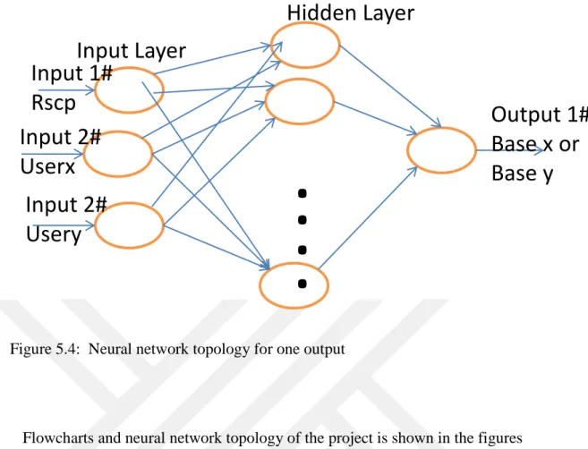
Figure 5.4: Neural network topology for one output
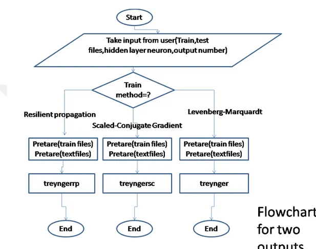
Flowcharts and neural network topology of the project is shown in the figures above. These figures explain the project flowchart simply and visually.
Figure 5.1 explains the flowchart for the 3 input 2 output network topology. It explains which methods will run if the user chooses 3 input 2 output network topology in its order. Neural network topology is represented in figure 5.2 visually. It briefly shows what inputs, hidden layer and outputs are taken. Figure 5.1 explains the flowchart for the 3 input 2 output network topology. It explains which methods will run if the user chooses 3 input 2 output network topology in its order. Neural network topology is represented in figure 5.2 visually. It briefly shows what inputs, hidden layer and outputs are taken.
Below methods of the project are explained. These methods are in the flowcharts. These methods benefit from open source library "Encog Library". Encog is a jar file that contains machine learning methods. Encog library is included in the java project to use its methods in source code. For example, if we want to create a network, we can call it by typing network1 = new BasicNetwork();.eThis creates a ready network from encog library. Furthermore, if we want to use a training method
Input Layer
Hidden Layer
Input 1#
Rscp
.
.
.
.
Output 1#
Base x or
Base y
Input 2#
Userx
Input 2#
Usery
42
it is enough to type LevenbergMarquardtTraining train = new
LevenbergMarquardtTraining(network1, trainingSet);
Dosyeokuma Project
Readdgertrain method
This method’s function is to take raw data and transform it into processed data. This raw data contains cellid,userx,usery,rscp,srcm,basex and basey. Basex and basey are prepared by user in excel or other programs. This raw data is prepared by user from cellphone data in excel other programs. After being prepared as comma seperated file. Program takes values from the file using comma as delimiter.
valus=line.split(",");
for(int i=0; i<valus.length; i++){ cellId=valus[0];
43 outputy=valus[2]; rscp=valus[3]; srcm=valus[4]; basex=valus[5]; basey=valus[6]; }
This processed data is put into a multidimensional array. Raw data contains longitude and latitude values in degree values. But we need meter values in order to train it. Therefore program makes a calculation and gives the point’s distance to (0,0) point at ecuador. Program parses the data and turns into numeric values in order to use the data.
longi= ((Double.parseDouble(outputx))) ; late=((Double.parseDouble(outputy))) ; baseym=(Double.parseDouble(basey)); baseym2=baseym*111; basexm=(Double.parseDouble(basex)); latee=(late*111); longii=longi*111.195; basexm2=basexm*111.195;
Program puts data into multidimensional array
xl1[ind][0]= Double.valueOf(cellId); xl1[ind][1] = longii; xl1[ind][2]= latee;
44 xl1[ind][4]=Double.valueOf(outputx); xl1[ind][5]=Double.valueOf(outputy); xl1[ind][6]=Double.valueOf(srcm); xl1[ind][7]=basexm2; xl1[ind][8]=baseym2;
Arfillgertrain method
This method’s function is to create an ordered multidimensional array. It continues the work that readdgertrain method started. It takes the array that readdgertrain method created and as output it makes it ordered according to cellids. And when doing this job it benefits from a basic algorithm. If it takes a cellid value, it scans the multidimensional array from beginning to end and signs them as false so that it doesn’t put it into unique cellid array. At the same time multidimensional array becomes ordered.
for (int i = 0; i < xl1.length; i++) { flag= xl1[i][0]; if(barray[i]==true){ z1[unind]=xl1[i][0]; unind++; }
45
//A cell-id value is read from the array and it is compared with other values //in the array. If it matches,this values are put into another array
// In addition boarray with this index is marked as false //Two for loops are used to go through arrays
//An array is required for unique cell ids for (int j = 0; j < xl1.length; j++) {
if(flag==xl1[j][0]&&barray[j]!=false){ yl1[indx][0]=xl1[j][0]; yl1[indx][1]=xl1[j][1]; yl1[indx][2]=xl1[j][2]; yl1[indx][3]=xl1[j][3]; yl1[indx][4]=xl1[j][4]; yl1[indx][5]=xl1[j][5]; yl1[indx][6]=xl1[j][6]; yl1[indx][7]=xl1[j][7]; yl1[indx][8]=xl1[j][8]; barray[j]=false; indx++; } } }
46
Objefillgertrain method
This method’s function is to create cell objects. These cell objects each have an unique cell id and in addition it has its own cell’s user longitude,latitude and rscp values. In short it has everthing necessary and important for the cell. It makes this according to a basic algorithm. It takes the unique cellid array and ordered multidimensional array. It traverses multidimensional array by cellids and takes all data related to that cell. Then it puts this data to a cell object. All necessary and important data is stored in that cell object. After an object is finished, it goes to next cell object that is in the object array.
for (int i = 0; i < xl1.length; i++) { myindex=0; while(xl1[i]==yl1[index][0]&&xl1[i]!=0){ obje1[i].cellId=yl1[index][0]; obje1[i].longitude[myindex]=yl1[index][1];
47 obje1[i].latitude[myindex]=yl1[index][2]; obje1[i].rscp[myindex]=yl1[index][3]; obje1[i].longer[myindex]=yl1[index][4]; obje1[i].latger[myindex]=yl1[index][5]; obje1[i].Scrm[myindex]=yl1[index][6]; obje1[i].basex[myindex]=yl1[index][7]; obje1[i].basey[myindex]=yl1[index][8]; myindex++; index++; if(xl1[i]==0) break; if(myindex>obje1[i].longitude.length) break; if(index>yl1.length) break; } }
Pretare method
public static void pretare (String path,double[][]input,double[][]target,double[]cellIdar, double[]lngavg, double[]latavg)
Pretare method takes 6 parameters as input. “String path” variable takes the file path of the file which is read.”double[][]input” is entered by program as a blank array. After the function processes this array, it is filled with x,y and rscp values.” double[][]target “variable is entered
48
by program as a blank array. After the function processes this array, it is filled with base x and base y values. “double[]cellIdar” variable is entered by program as a blank array. After the function processes this array, it is filled with cell-id list.” double[]lngavg” is a blank array entered by program. After the function processes this array, it is filled average longitude value of a specific cell.” double[]latavg” is a blank array entered by program. After the function processes this array, it is filled average latitude value of a specific cell.Algorithm logic is similar in pretare1inp method.
GUI class or main class that called myproject class’ pretare method uses static arrays for use in method. These filled in static arrays are then used for other methods. Pretare method takes three arrays and one string as arguments. String path specifies the location of the file that will be read. A line is read,then it is divided into pieces by a delimiter. Zero index piece becomes the cell id of the data,first will be x coordinate of user, second will be y coordinate of user, third will be rscp value of the user gsm. Fourth will be the x coordinate of the base station and fifth will be the y coordinate of the base station.
valus=line.split(";");
for(int i=0; i<valus.length; i++){ cell=valus[0]; outputx=valus[1]; outputy=valus[2]; rscp=valus[3]; desiredx=valus[4]; desiredy=valus[5]; }
Zero index data piece will be put into cellid array. This cellid array will not be used for training but will be used for report later. First, second and third values will be put into multidimensional input array. Fourth and fifth data pieces will be used for multidimensional target array. Input and target arrays will be used for training and testing. They are also needed in reports as well. Pieces are strings. By DoubleValueOf method they’re converted to double values. There is an algorithm that distinguishes distinct cellid values.