Search for resonances decaying to a pair of Higgs bosons in the b b ¯ q q ¯ ’ℓν final state in proton-proton collisions at √s = 13 TeV

JHEP10(2019)125

Published for SISSA by Springer

Received: April 8, 2019 Revised: August 12, 2019 Accepted: September 10, 2019 Published: October 9, 2019

Search for resonances decaying to a pair of Higgs

bosons in the bbqq

0

`ν final state in proton-proton

collisions at

√

s = 13 TeV

The CMS collaboration

E-mail: cms-publication-committee-chair@cern.ch

Abstract: A search for new massive particles decaying into a pair of Higgs bosons in

proton-proton collisions at a center-of-mass energy of 13 TeV is presented. Data were

collected with the CMS detector at the LHC, corresponding to an integrated luminosity

of 35.9 fb−1. The search is performed for resonances with a mass between 0.8 and 3.5 TeV

using events in which one Higgs boson decays into a bottom quark pair and the other decays into two W bosons that subsequently decay into a lepton, a neutrino, and a quark pair. The Higgs boson decays are reconstructed with techniques that identify final state quarks as substructure within boosted jets. The data are consistent with standard model expectations. Exclusion limits are placed on the product of the cross section and branching fraction for generic spin-0 and spin-2 massive resonances. The results are interpreted in the context of radion and bulk graviton production in models with a warped extra spatial dimension. These are the best results to date from searches for an HH resonance decaying to this final state, and they are comparable to the results from searches in other channels for resonances with masses below 1.5 TeV.

Keywords: Beyond Standard Model, Hadron-Hadron scattering (experiments), Higgs physics

JHEP10(2019)125

Contents 1 Introduction 1 2 The CMS detector 2 3 Simulated samples 3 4 Event reconstruction 4

4.1 Electron and muon identification 4

4.2 Jet clustering and momentum corrections 5

4.3 Hadronic boson decay reconstruction 6

4.4 Jet flavor identification 7

4.5 Semileptonic Higgs boson decay and signal mass reconstruction 7

5 Event selection and categorization 7

5.1 Event selection 7

5.2 Event categorization 8

5.3 Control region event selection and categorization 10

6 Background and signal modeling 11

6.1 Background categorization 11

6.2 Template creation strategy 11

6.3 Background process modeling 12

6.4 Signal process modeling 13

6.5 Validation of background models with control region data 14

7 Systematic uncertainties 14

7.1 Background normalization uncertainties 16

7.2 Background shape uncertainties 16

7.3 Signal uncertainties 18

8 Results 18

9 Summary 21

The CMS collaboration 34

1 Introduction

The discovery of a Higgs boson (H) [1–3] established the existence of at least a simple mass

generation mechanism for the standard model (SM) [4,5], the so-called “Higgs Mechanism”.

The simple model, however, has a number of limitations that are ameliorated [6] by a

so-called “extended Higgs sector”. Supersymmetry [7–14] requires such an extended Higgs

sector, with new spin-0 particles. Another class of models with warped extra dimensions,

proposed by Randall and Sundrum [15], postulates the existence of a compact fourth spatial

JHEP10(2019)125

a tower of Kaluza-Klein excitations, leading to possible spin-0 radions [16–19] or spin-2 bulk

gravitons [20–22]. The ATLAS [23–38] and CMS [39–57] collaborations have conducted a

number of searches for these particles, where the new bosons decay into vector bosons and/or Higgs bosons (WW, ZZ, WZ, HH, ZH, or WH).

In this paper, we describe a search for narrow resonances (X) decaying to HH, where one H decays to a bottom quark pair (bb ) and the other decays to a W boson pair, with at

least one W boson off-shell (WW∗). These are the most likely and second-most likely Higgs

boson decay channels, respectively. The otherwise large SM background of jets produced via quantum chromodynamics processes, referred to as “multijet” background, is greatly

reduced by considering the WW∗ final state in which one W boson decays to quarks (qq0)

and the other to either an electron-neutrino pair (eν) or a muon-neutrino pair (µν). This

search is optimized for particle mass m_X > 0.8 TeV and employs new techniques for this

channel to recognize substructure within boosted jets. The search is performed on a data set collected in 2016 at the CERN LHC, corresponding to an integrated luminosity of

35.9 fb−1 of proton-proton (pp) collisions at √s = 13 TeV.

The Higgs bosons have a high Lorentz boost because of the large values of mX

consid-ered, and the decay products of each one are produced in a collimated cone. The H → bb decay is reconstructed as a single jet, referred to as the bb jet, with high transverse

mo-mentum pT. The H → WW

∗

decay is also reconstructed as a single jet, referred to as the

qq0 jet, but with a nearby lepton (e or µ). In both cases, the jets are required to have

a reconstructed topology consistent with a substructure arising from a boson decaying to two quarks. The semileptonic Higgs boson decay chain is reconstructed from both the visible decay products and the missing transverse momentum. A distinguishing

character-istic of the signal is a peak in the two-dimensional plane of the bb jet mass m_bb and the

reconstructed HH invariant mass m_HH.

The main SM background to this search arises from top quark pair tt production in which one top quark decays via a charged lepton (t → Wb → `νb) and the other decays

exclusively to quarks (t → Wb → qq0b). The top quarks affecting this analysis have decay

products that are collimated because of large boosts. In particular, the all-hadronic top

quark decays can be misreconstructed as single bb jets. Peaks in the m_bb distribution

from this background correspond to fully contained top quark and W boson decays. The second-largest background is primarily composed of production of W bosons in association with jets (W + jets) and multijet events. Both W + jets and multijet background events

are experimentally distinct from tt production, in part because their m_bb distributions are

smoothly falling.

In this analysis, the events are divided into 12 exclusive categories by lepton flavor,

qq0jet substructure, and bb jet flavor identification. The SM background and signal yields

are then simultaneously estimated using a maximum likelihood fit to the two-dimensional

distribution in the m_bb and m_HH mass plane.

2 The CMS detector

The central feature of the CMS apparatus is a superconducting solenoid of 6 m internal diameter, providing a magnetic field of 3.8 T. Within the solenoid volume are a silicon pixel

JHEP10(2019)125

and strip tracker, a lead tungstate crystal electromagnetic calorimeter (ECAL), and a brass and scintillator hadron calorimeter (HCAL), each composed of a barrel and two endcap sections. Forward calorimeters extend the coverage in pseudorapidity η provided by the barrel and endcap detectors. Muons are detected in gas-ionization chambers embedded in the steel flux-return yoke outside the solenoid. Events of interest are selected using a

two-tiered trigger system [58]. The first level, composed of custom hardware processors, uses

information from the calorimeters and muon detectors to select events at a rate of around 100 kHz within a time interval of less than 4 µs. The second level, known as the high-level trigger, consists of a farm of processors running a version of the full event reconstruction software optimized for fast processing, and reduces the event rate to around 1 kHz before data storage. A more detailed description of the CMS detector, together with a definition

of the coordinate system used and the relevant kinematic variables, can be found in ref. [59].

3 Simulated samples

Signal and background yields are extracted from data with a fit using templates of the

two-dimensional m_bb and m_HH mass distribution. The signal and background templates

are obtained from samples generated using Monte Carlo simulation.

The signal process pp → X → HH → bb WW∗ is simulated for both the spin-0 and

spin-2 resonance scenarios. The X bosons are produced via gluon fusion and have a 1 MeV resonance width, which is small compared to the experimental resolution. The samples

are generated at leading order (LO) using the MadGraph5 amc@nlo 2.2.2 generator [60]

with MLM merging [61] for mX between 0.8 and 3.5 TeV.

The background processes are produced with a variety of generators. The same gen-erator as for signal is used to produce tt , W + jets, multijet, Higgs boson production in association with a t quark (tH), and Drell-Yan samples. Samples of WZ diboson pro-duction and the associated propro-duction of tt with either a W or Z boson (tt + V) are also generated with MadGraph5 amc@nlo, but at next-to-leading-order (NLO) with the

FxFx jet merging scheme [62]. The WW diboson process, single top production, and tt H

are generated with powheg v2 at NLO [63–70]. Single top in the associated production

(tW) and t-channel (tq) processes are included, but not s-channel (tb), which is negligible. For all samples, the parton showering and hadronization are simulated with pythia

8.205 [71] using the CUETP8M1 [72] tune, with NNPDF 3.0 [73] parton distribution

func-tions (PDFs). The simulation of the CMS detector is performed with the Geant4 [74]

toolkit. Additional pp collisions in the same or nearby bunch crossings (pileup) are sim-ulated and the samples are weighted to have the same pileup multiplicity as measured in data.

While the final background normalizations are extracted from data with the template fit, all processes are initially normalized to their theoretical cross sections, using the highest order available. The tt process is rescaled to the next-to-next-to-leading-order (NNLO)

cross section, computed with Top++ v2.0 [75]. The W +jets and Drell-Yan samples are

also normalized using NNLO cross sections, but calculated with fewz v3.1 [76]. NLO cross

JHEP10(2019)125

79]. The multijet and tt + V cross sections are obtained from MadGraph5 amc@nlo

at LO and NLO accuracy, respectively. NLO cross sections are used for the tt H and tH

processes [80].

4 Event reconstruction

Signal events and those from the primary SM background source, tt production with a

single-lepton final state, have similar signatures. Both processes feature high-pT jets with

substructure consistent with two or more quarks, jets containing b hadron decays, and leptons that originate from a W boson decay. Additional discrimination of signal events from background events is achieved by associating the lepton and each jet with a particle

in the HH → bb WW∗→ bb`νqq0 decay chain and applying mass constraints.

A particle-flow (PF) algorithm [81] aims to reconstruct and identify each individual

particle in an event, with an optimized combination of information from the various ele-ments of the CMS detector. The reconstructed vertex with the largest value of summed

tracking-object p2_T is taken to be the primary pp interaction vertex. These tracking objects

are track jets and the negative vector sum of the track jet p_T. Track jets are clustered

using the anti-kT jet finding algorithm [82,83] with the tracks assigned to the vertex as

inputs.

4.1 Electron and muon identification

Events are required to have exactly one isolated lepton. This lepton is associated with the

leptonic W boson decay. Reconstructed electrons are required to have p_T > 20 GeV and

|η| < 2.5, and are identified with a high-purity selection to suppress the potentially large

multijet background [84]. Muons are required to have pT > 20 GeV and |η| < 2.4, and

to pass identification criteria optimized to select muons with >95% efficiency [85]. The

impact parameter of lepton tracks with respect to the primary vertex is required to be con-sistent with originating from that vertex: longitudinal distance <0.1 cm, transverse distance <0.05 cm, and significance <4 standard deviations of the three-dimensional displacement. These criteria remove background events where the lepton is produced by a semileptonic heavy-flavor decay rather than a W boson decay. In addition, these criteria prevent incor-rectly selecting a lepton from a heavy-flavor decay in signal events. Requiring leptons to be isolated from nearby hadronic activity is important to suppress background, but can also cause significant signal inefficiency because of the collinear decay of the Lorentz-boosted Higgs boson. This inefficiency is mitigated by using an isolation definition specifically

de-signed for leptons from boosted decays [86]. The isolation metric Irel is the pT sum of the

PF particles with ∆R < ∆R_iso with respect to the lepton, divided by the lepton p_T. The

angular distance is ∆R =p(∆η)2+ (∆φ)2. The value ∆R_iso is defined to be

∆R_iso =        0.2, pT< 50 GeV, 10 GeV/p_T, 50 < p_T < 200 GeV, 0.05, p_T> 200 GeV, (4.1)

JHEP10(2019)125

which preserves signal efficiency even in the case of high m_X. The neutral particle

contribu-tion to Irel from pileup interactions is estimated and removed using the method described

in ref. [84]. Electrons are selected with I_rel < 0.1, whereas muons, because of lower

back-ground rates, are selected with I_rel< 0.2.

Muons in signal events have an approximate efficiency of 85% for mX = 0.8 TeV,

de-creasing to 70% for m_X = 3.5 TeV, with isolation being the leading source of inefficiency

compared to all other requirements. The efficiency to select electrons is lower,

approxi-mately 40% for mX = 0.8 TeV, decreasing to 6% for mX = 3.5 TeV. The leading source of

electron inefficiency is a selection imposed at the reconstruction level on the ratio of the energy deposited in the HCAL to that deposited in the ECAL. Signal electrons typically fail this selection because of the nearby energy deposits from the hadronic W boson decay. Lepton reconstruction, identification, and isolation efficiencies are measured in a Z → ``

data sample with a “tag-and-probe” method [87] and the simulation is corrected for any

discrepancies with the data. There is generally much less hadronic activity in Z → `` events than in signal events, so these corrections are parameterized by nearby hadronic activity to ensure their applicability. For this measurement, a lepton’s hadronic activity is quantified by using the PF particles with ∆R < 0.4 about the lepton to obtain two

variables: the relative p_T sum around the lepton and the ∆R between the lepton and the

~

p sum of these particles. When parameterized by these two variables, a similar drop in efficiency is measured in low ∆R and high relative momentum Z → `` events as in signal events. The lepton selection efficiencies in simulation are found to be within 10% of those in data. The uncertainty in the correction is at its largest for high hadronic activity, with a maximum value of 10% for electrons and 5% for muons.

4.2 Jet clustering and momentum corrections

Two types of jets are used. Because the X bosons being considered here are much more massive compared to the mass of the Higgs bosons they decay into, the subsequent H → bb

and W → qq0 decays are each reconstructed as single, merged jets. These jets are formed

by clustering PF particles according to the anti-k_T algorithm [82, 83] with a distance

parameter of 0.8, and are referred to as AK8 jets. The PF particle or particles associated with the lepton are not included in the clustering of this jet type in order to prevent

the qq0 jet from containing the lepton’s momentum. Jets of the second type, referred to

as AK4 jets, are used to suppress background events from tt production by identifying additional jets originating from b quarks. These jets are also clustered according to the

anti-k_T algorithm, but with a distance parameter of 0.4. Jets of both types are required

to have |η| < 2.4 so that a majority of their area is within acceptance of the tracker. The

AK8 jets are required to have p_T > 50 GeV, whereas the threshold is 20 GeV for AK4 jets.

Jet momentum for both jet types is determined as the vectorial sum of all particle momenta in the jet, and is found from simulation to be, on average, within 5 to 10% of

the true momentum over the whole p_T spectrum and detector acceptance. Additional pp

interactions within the same or nearby bunch crossings can contribute additional tracks and calorimetric energy depositions, increasing the apparent jet momentum. The pileup

JHEP10(2019)125

at the reconstructed particle-level, making use of local shape information, event pileup properties, and tracking information. Charged particles identified to be originating from pileup vertices are discarded. For each neutral particle, a local shape variable is computed using the surrounding charged particles compatible with the primary vertex within the tracker acceptance (|η| < 2.5), and using both charged and neutral particles in the region outside of the tracker coverage. The momenta of the neutral particles are then rescaled according to their probability to originate from the primary interaction vertex deduced

from the local shape variable [89]. Jet energy corrections are derived from simulation

studies so that the average measured response of jets becomes identical to that of particle level jets. In situ measurements of the momentum balance in dijet, photon+jet, Z+jet, and multijet events are used to determine any residual differences between the jet energy scale

in data and in simulation, and appropriate corrections are made [90]. Additional selection

criteria are applied to each jet to remove jets potentially dominated by instrumental effects

or reconstruction failures [89].

4.3 Hadronic boson decay reconstruction

In high-mXsignal events, the H → WW

∗

decay is reconstructed as an AK8 jet and a nearby lepton, with the jet itself containing two localized energy deposits, “subjets”, one from each

quark. Only the AK8 jet closest in ∆R to the lepton is considered for qq0jet reconstruction.

This jet satisfies qq0 jet reconstruction criteria if it is close to the lepton (∆R < 1.2) and

if two subjets with p_T > 20 GeV and |η| < 2.4 can be identified. The constituents of the

jet are first reclustered using the Cambridge-Aachen algorithm [91, 92]. The “modified

mass drop tagger” algorithm [93,94], also known as the “soft drop” (SD) algorithm, with

angular exponent β = 0, soft cutoff threshold z_cut < 0.1, and characteristic radius R₀ =

0.8 [95], is applied to remove soft, wide-angle radiation from the jet. The subjets used

in the analysis are those remaining after the algorithm has removed all recognized soft

radiation. The purity of the qq0 jet reconstruction is quantified using the “N -subjettiness”

variables τ_N, which measure compatibility with the hypothesis that a jet originates from N

subjets [96]. The τN are obtained by first reclustering the jet into N subjets using the kT

algorithm [97]. The variables are then calculated with these subjets as described in ref. [96]

with a characteristic radius R0= 0.8. The ratio of N -subjettiness variables, τ2/τ1, is used

to discriminate qq0 jets originating from two-pronged W boson decays against those from

single quarks or gluons.

Generally, the Higgs bosons in signal events have large Lorentz boosts and are produced with ∆φ ≈ π between them. Therefore, bb jet candidates are required to be AK8 jets with

∆φ > 2 from the lepton and ∆R > 1.6 from the qq0 jet. If there are two or more bb jet

candidates, the one leading in pT is used. This jet is reconstructed as a bb jet if it is the

leading or second-leading AK8 jet in p_T, has p_T> 200 GeV, and if two constituent subjets

with p_T > 20 GeV and |η| < 2.4 can be identified. The bb jet SD mass, which is the

invariant mass of the two subjets, is used to obtain m_bb. The mass grooming helps reject

events for which the bb jet originates from a single quark or gluon. The performance of

JHEP10(2019)125

applied as a function of p_T to make the average m_bb value be 125 GeV, the Higgs boson

mass mH [98].

4.4 Jet flavor identification

Jets and subjets are identified as likely to have originated from b hadron decays using

the combined secondary vertex b tagging algorithm [99]. Two operating points of the

algorithm are used, which have similar performance on subjets and AK4 jets. A high-efficiency working point, referred to as “loose”, has an high-efficiency of ≈80% and a light-quark or gluon misidentification rate of ≈10%. The “medium” operating point has an efficiency and misidentification rate of ≈60% and ≈1%, respectively. A “tight” operating point is not

used. Jets or subjets with pT > 30 GeV and |η| < 2.4 are considered for b tagging. This

lower bound on p_T is chosen because the uncertainty in b tagging calibrations is larger for

lower p_T jets and because the b quarks in our signal events have large p_T. The b tagging

efficiency and misidentification rate are measured in data, and the simulation is corrected

for any discrepancy [99].

4.5 Semileptonic Higgs boson decay and signal mass reconstruction

The missing transverse momentum vector ~pTmiss is computed as the negative vector pT sum

of all the PF candidates in an event [100]. The ~p_Tmiss is modified to account for corrections

to the energy scale of the reconstructed jets in the event. The ~p_Tmiss is an estimate of the

transverse momentum of the neutrino in the semileptonic Higgs boson decay chain. The

longitudinal momentum p_z of this neutrino is estimated by setting the invariant mass of

the neutrino, the lepton, and the qq0 jet to mHand solving the corresponding second-order

equation. If two real solutions exist, the one with the smaller magnitude is chosen. If the

p_z solution is complex, the real component of the solution is used. Other methods for

determining the neutrino pz, including choosing the other pz solution or incorporating the

imaginary components, do not improve the m_HHresolution. The reconstructed momentum

of the W boson that decays to leptons, referred to as the `ν candidate, is obtained from

the lepton and the estimated neutrino momenta. The WW∗ candidate momentum is then

obtained from the combined `ν candidate and the qq0 jet momenta. The invariant mass of

this object and the bb jet is m_HH.

5 Event selection and categorization

Events are included in this search if they pass the following criteria that indicate they originate from a X boson decay and are then divided into 12 independent categories. A separate set of criteria is used to define control regions, which are used to validate the modeling of background processes.

5.1 Event selection

Events are selected by the trigger system if they contain one of the following: an isolated

electron with p_T > 27 GeV, an isolated muon with p_T> 24 GeV, or H_T > 800 GeV (900 GeV

for the last quarter of data taking), where H_T is the scalar sum of jet p_T for all AK4

JHEP10(2019)125

used because the online lepton isolation selection is inefficient for high-m_X signal, which

provides two high-pT, collimated Higgs boson decays. These events have large HT and

are instead selected with higher efficiency by the H_T trigger. Additional multi-object

triggers that select events with a single lepton and H_T > 400 GeV supplement these two

single-object triggers, thereby maintaining high signal trigger efficiency for the entire mX

analysis range. The pileup correction for H_T is the same offline as in the trigger. The

trigger efficiency is measured for tt events in data and is >94% for events passing HT and

lepton pT offline selection criteria. The simulation is corrected so that its trigger efficiency

matches the efficiency measured with data. The trigger efficiency for signal events is 98%

for mX = 0.8 TeV and >99% for mX > 1 TeV.

Offline, events are required to have H_T > 400 GeV and a lepton with p_T > 30 GeV

for electrons and p_T> 26 GeV for muons. Background events from Z → `` are suppressed

by rejecting events that contain additional leptons with pT > 20 GeV. Events are further

required to have a qq0 jet and a bb jet. Background from tt production is reduced by

vetoing events with AK4 jets that are ∆R > 1.2 from the bb jet and pass the medium b tagging operating point.

Jets in multijet and W + jets events tend to be produced at higher |η| than those produced in signal events, which contain jets from the decay of a heavy resonance. The

ratio pT/m, which is the WW

∗

candidate pT divided by mHH, exploits this property

and is especially effective at high m_HH. Events are required to have p_T/m > 0.3. A

m_H constraint on the WW∗ candidate is not useful because it is already imposed in the

neutrino momentum calculation. However, there is discrimination because the decay chain

involves a two-body decay as an intermediate step. We define a variable m_D ≡ p_T∆R/2,

where ∆R is the separation of the two reconstructed W bosons and the pT is that of the

WW∗candidate. This variable is based on an approximate expression for the opening angle

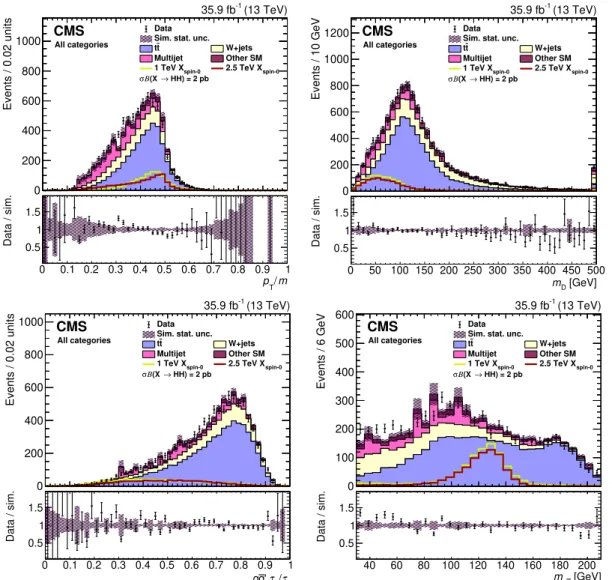
of a highly boosted, massive particle decay. The selection m_D< 125 GeV is applied and has

a high efficiency for signal events. The mD and pT/m distributions are shown in figure 1.

This figure is shown only to illustrate how these variables are used to discriminate signal events from background events; the simulated distributions are pre-modeling and pre-fit.

The initial difference in m_bb near 50 GeV between simulation and data is apparent only

with the pre-fit background model; with the full post-fit background model no discrepancy appears.

5.2 Event categorization

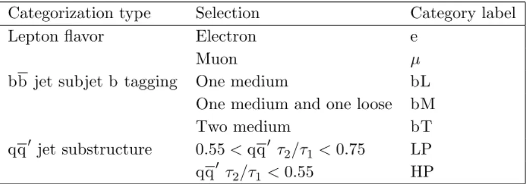
Events are categorized by event properties that reflect the signal purity. The categorization

allows for a single set of selections that targets the full mX range, which is preferable to

search categories that are optimized for different mass ranges. Electron and muon events are separated because their efficiencies for background and signal are different, resulting in different signal purities. The electron and muon categories are labeled “e” and “µ”, respectively, in the figures. There are three categories of b tagging, evaluated by counting the number of subjets in the bb jet that pass b tagging operating points. The first, labeled “bL”, is composed of events in which one subjet passes the medium operating point and the other does not pass the loose operating point. Events with one subjet passing the medium

JHEP10(2019)125

0 200 400 600 800 1000 Events / 0.02 units (13 TeV) -1 35.9 fb CMS All categories HH) = 2 pb → (X Β σ Data Sim. stat. unc.

t

t W+jets

Multijet Other SM

spin-0

1 TeV X 2.5 TeV Xspin-0

0 0.1 0.2 0.3 0.4 0.5 0.6 0.7 0.8 0.9 1 m / T p 0.5 1 1.5 Data / sim. 0 200 400 600 800 1000 1200 Events / 10 GeV (13 TeV) -1 35.9 fb CMS All categories HH) = 2 pb → (X Β σ Data Sim. stat. unc.

t

t W+jets

Multijet Other SM

spin-0

1 TeV X 2.5 TeV Xspin-0

0 50 100 150 200 250 300 350 400 450 500 [GeV] D m 0.5 1 1.5 Data / sim. 0 200 400 600 800 1000 Events / 0.02 units (13 TeV) -1 35.9 fb CMS All categories HH) = 2 pb → (X Β σ Data Sim. stat. unc.

t

t W+jets

Multijet Other SM

spin-0

1 TeV X 2.5 TeV Xspin-0

0 0.1 0.2 0.3 0.4 0.5 0.6 0.7 0.8 0.9 1 1 τ / 2 τ ' q q 0.5 1 1.5 Data / sim. 0 100 200 300 400 500 600 Events / 6 GeV (13 TeV) -1 35.9 fb CMS All categories HH) = 2 pb → (X Β σ Data Sim. stat. unc.

t

t W+jets

Multijet Other SM

spin-0

1 TeV X 2.5 TeV Xspin-0

40 60 80 100 120 140 160 180 200 [GeV] b b m 0.5 1 1.5 Data / sim.

Figure 1. Pre-modeling and pre-fit distributions of the discriminating variables, which are de-scribed in the text, are shown for data (points) and SM processes (filled histograms) as predicted directly from simulation. The statistical uncertainty of the simulated sample is shown as the hatched band. The solid lines correspond to spin-0 signals for mX of 1 and 2.5 TeV. The product of the cross section and branching fraction to two Higgs bosons is set to 2 pb for both signal models. The lower panels show the ratio of the data to the sum of all background processes.

operating point and one passing the loose but not the medium operating point are denoted “bM”, and those with two subjets passing the medium operating point are labeled “bT”.

The final categorization is based on the τ2/τ1 N -subjettiness ratio of the qq

0

jet, referred

to as qq0 τ₂/τ₁. Events with 0.55 < qq0 τ₂/τ₁ < 0.75 fall into the low-purity category,

“LP”, while those with qq0 τ2/τ1 < 0.55 are included in a high-purity category, “HP”.

The qq0 τ₂/τ₁ distribution is shown in figure 1. Events are divided into all combinations

of categories for a total of 12 exclusive selections. When describing a single selection, the category label is a combination of those listed above. For example, the tightest b tagging

category with a low-purity qq0 τ₂/τ₁ selection in the electron channel is: “e, bT, LP”. The

JHEP10(2019)125

Categorization type Selection Category label

Lepton flavor Electron e

Muon µ

bb jet subjet b tagging One medium bL

One medium and one loose bM

Two medium bT

qq0 jet substructure 0.55 < qq0 τ₂/τ₁< 0.75 LP

qq0 τ₂/τ₁< 0.55 HP

Table 1. Event categorization and corresponding category labels. All combinations of the two lepton flavor, three bb jet subjet b tagging, and two qq0 jet substructure selections are used to form 12 independent event categories. For the bb jet subjet b tagging type, “medium” refers to the subjets that pass the medium b tagging operating point and “loose” refers to those that pass the loose, but not the medium, operating point.

The search is performed in these categories for 30 < m_bb < 210 GeV. Events below

30 GeV would provide little sensitivity and would be relatively difficult to model since these are events for which the SD algorithm results in nearly all of the jet energy being removed.

The m_bb distribution is displayed in figure 1. Events with 700 < m_HH < 4000 GeV are

analyzed. The lower bound is chosen such that the mHH distribution is monotonically

decreasing for background events. The upper bound is far above the highest mass event

observed in data. For spin-0 scenarios, the selection efficiency for X → bb qq0`ν events to

pass the criteria of any event category is 9% at mX = 0.8 TeV. The efficiency increases with

m_X to 18% at m_X = 1.2 TeV because the Higgs boson decays become more collimated.

Above 1.2 TeV the selection efficiency decreases to a minimum of 9% at m_X = 3.5 TeV

because of the combination of lower b tagging efficiency for high-pT jets and the worsening

of the lepton isolation for extremely collimated Higgs boson decays. The Higgs bosons in spin-2 signal events are more central in polar angle than those from spin-0 signal, resulting in a larger selection efficiency, ≈15%, relative.

5.3 Control region event selection and categorization

Two control regions are used to validate the SM background estimation and to obtain systematic uncertainties. The first, labeled “tt CR”, targets backgrounds with top quarks, specifically tt production. Such events are selected by inverting the AK4 jet b-tagging

veto. The m_D and p_T/m selections are removed to increase the statistical power of the

sample. This control region is then divided into the 12 categories previously described.

Overall, the m_bb and m_HH shapes in this control region are very similar to the shapes in

the signal region for the backgrounds that contain top quarks. The top quark pT spectrum

in tt events has been shown to be mis-modelled in simulation [101, 102]. A correction

is measured in this region and applied to the simulation as a normalization correction. However, ultimately the final value of the normalization and its uncertainty come from the two-dimensional fit to signal and background. While the tt CR is an adequate probe of processes that involve top quarks, it is not sensitive to the multijet or W+jets backgrounds.

JHEP10(2019)125

Instead, a second control region, labeled “q/g CR”, is used to study the modeling of the mass shapes and the relative composition of the W + jets and the multijet backgrounds, which is similar to their relative composition in the search region. The selection of events in this control region is the same as for the signal region, except that the bb jet is required to have no subjets passing the loose b tagging operating point. As a result, the events in this control region are not categorized by bb jet b tagging, but are still categorized by

lepton flavor and qq0 τ2/τ1.

6 Background and signal modeling

The search is performed by simultaneously estimating the signal and background yields using a maximum likelihood fit to the data in the 12 event categories. The data are binned

in two dimensions, m_HH and m_bb, with the ranges specified in section5and with bin widths

of 25 and 2 GeV, respectively. The bin widths are smaller than the mass resolutions, but large enough to keep the number of bins computationally tractable. Each processes is modeled with two-dimensional templates, one for each event category. The templates are created using simulation. Because of the limited size of the simulated samples, we employ methods to smooth the background distributions. Shape uncertainties that account for possible differences between data and simulation are included while executing the fit. This

fitting method was previously presented in ref. [52].

6.1 Background categorization

Background events are separated into four generator-level categories, each with distinct

m_bb shapes. The categories are defined by counting the number of generator-level quarks

from the immediate decay of a top quark, W boson, or (rarely) Z boson within ∆R < 0.8

of the bb jet axis. The first, labeled “m_t background”, is the component in which all

three quarks from a single top quark decay fulfill this criterion. The second is labeled

“mW background” and consists of those events that are not labeled mt background but in

which both quarks from a W or Z boson fall within the jet cone. Both of these backgrounds

contain resonant peaks in the m_bb shape corresponding to either the top quark or W boson

mass. The “lost t/W background” contains events with partial decays within the bb jet, identified as events in which at least one quark is contained within the jet cone, but does not satisfy one of the previous two requirements. The last category, “q/g background”, desig-nates all other events. The first three categories are primarily composed of tt events, while the last is a composite of W+jets, multijet, and tt events. The background categorization

is summarized in table 2.

6.2 Template creation strategy

A template is produced for each of the 12 event categories, for each of the four back-grounds. To reduce statistical fluctuations in the templates, each is generated from an initial smooth template created by relaxing requirements or by combining categories. In all cases, the regions with relaxed criteria are chosen such that the shapes for these regions are similar to those for the full event selection. The final template for each event category

JHEP10(2019)125

Bkg. category Dominant SM process(es) Resonant in m_bb Num. of gen.–level quarks

mt tt Yes (near mt) 3 from t

mW tt Yes (near mW) 2 from W

Lost t/W tt No 1 or 2

q/g W +jets and multijet No 0

Table 2. The four exclusive background categories with their kinematical properties and defining number of generator-level quarks within ∆R < 0.8 of the bb jet axis.

and background is produced by fitting the high-statistics template to the simulated sam-ples for that category’s event selection. The fit is performed in a similar manner to the fit to data and with a similar parameterization of the template shape. The templates are compared to simulation after applying the full event selection and any deviations in shape are found to be much smaller than the statistical uncertainty of the data sample. The background templates and associated systematic uncertainties are ultimately validated by

fitting to data in dedicated control regions, which is described in section 6.5.

While this procedure increases the statistical power of the simulation samples, the multijet background simulation sample cannot be produced with a large enough effective integrated luminosity to be directly used in the template creation. Instead, the similarity

of m_bb reconstruction for W +jets and multijet events is exploited. Both these processes

have bb jets that are composed of at least one quark or gluon that is misidentified as

a bb jet, resulting in nearly identical monotonically falling m_bb shapes. Both processes

also have similar relative fractions in the bL, bM, and bT categories. The W + jets and

multijet samples are used to obtain a combined yield and mHH distribution for each lepton

flavor and qq0 τ₂/τ₁ category. The m_bb modeling and the relative bb jet subjet b tagging

categorization is then taken from the W+jets sample. These two components are combined to form a single background shape when forming the q/g background templates.

6.3 Background process modeling

The background templates are modeled as conditional probabilities of m_bb as a function

of m_HH so that the templates include the correlation of these two variables. The

two-dimensional probability distribution is

Pbkg(mbb, mHH) = Pbb(mbb|mHH, θ1)PHH(mHH|θ2), (6.1)

where PHH and Pbb are one-dimensional probability distributions and the θ1 and θ2 are

nuisance parameters used to account for shape uncertainties. A parametric function that

models the full mHH range for background events is difficult to obtain from first

prin-ciples. Instead, a non-parametric approach is taken. The P_HH are produced from the

one-dimensional m_HH histograms with kernel density estimation (KDE) [103–105]. The

smoothing of the PHH distributions is controlled by parameters within the KDE

frame-work called bandwidths. Gaussian kernels with adaptive bandwidths are used because the

JHEP10(2019)125

is not suitable for the full distribution. These adaptive bandwidths depend on a first

iter-ation estimate of PHH, which itself is produced with KDE. However, for this first iteration

a global bandwidth h is used that scales as

h ∝ ( Pn i=1wi) 2 Pn i=1w 2 i !−1/5 . (6.2)

The sums are over all events in the simulation sample and the wi are the individual event

weights. This formulation is chosen to minimize the mean integrated squared error of the

estimate. For the adaptive estimates, the bandwidths h_i associated with each event are

h_i = h g

e

f (x_i)

!1/2

, (6.3)

where the ef (xi) are the estimated event densities at the location xi of the event and g is a

normalization factor such that the global bandwidth scale is controlled by h. As discussed

in ref. [106], adaptive KDE can result in overestimation of the distribution tails in the case

of large bandwidths being applied. This is ameliorated by imposing a maximum bandwidth value, which is usually chosen to be 1–5 times larger than the median bandwidth. The

mHH tail is further smoothed by fitting with an exponential function for mHH & 2 TeV.

The P_bb distributions are obtained for the m_t and m_W backgrounds by fitting m_bb

histograms with a double Crystal Ball function [107, 108]. This function has a Gaussian

core, which is used to model the bulk of the m_bb distribution, and power-law tails, which

describe the effects of more severe jet misreconstruction. The fits are performed for events

binned in m_HH to capture the evolution of the m_bb shape with m_HH. The double Crystal

Ball function parameters are then interpolated between mHH bins. The Pbb distributions

for the lost t/W and q/g backgrounds are estimated from the two-dimensional histograms with two-dimensional KDE. Independent adaptive bandwidths and bandwidth upper limits

are used for each dimension when forming the P_bb. Similar to the derivation of the PHH,

the m_HH tails are smoothed with exponential function fits. Simulation yields are used as

the initial values of the background yields in the fit to data.

6.4 Signal process modeling

The signal templates are also modeled as conditional probabilities

Psignal(mbb, mHH|mX) = PHH(mHH|mbb, mX, θ1)Pbb(mbb|mX, θ2). (6.4)

The Psignal distributions are first obtained for discrete mX values by fitting histograms of

the signal mass distributions. Models continuous in m_Xare then produced by interpolating

the fit parameters. The P_bb distributions are created by fitting m_bb histograms with a

double Crystal Ball function, and the resonance resolution is ≈10%. The shape for the bL categories also includes an exponential function to model the small fraction of signal events with no resonant peak in the distribution.

The P_HH distributions are also modeled with a double Crystal Ball function, but with

JHEP10(2019)125

are the mean and standard deviation parameters from the fit to m_bb, respectively. The

variable µHH, the mean of the Crystal Ball function, is then

µ_HH = µ₀(1 + µ₁∆_bb), (6.5)

where µ0 and µ1 are fit parameters. This parameterization models the characteristic that

a mismeasurement of the bb jet results in a mismeasurement of m_HH. The standard

deviation of mHH, denoted as σHH, also depends on mbb,

σ_HH =

(

σ₀(1 + σ₁|∆_bb|), ∆_bb < 0,

σ₀, ∆_bb > 0, (6.6)

where σ₀ and σ₁ are fit parameters. An undermeasurement of m_bb can be caused by

the SD algorithm removing energy from the Higgs boson decay. In such a scenario, the

correlation between the two variables worsens and the mHH resolution becomes wider. For

|∆_bb| > 2.5, only the values at the boundary are used since the correlation does not hold

for severe mismeasurements. The m_HH resolution is ≈6% for m_X = 1 TeV, decreasing to

4% for mX= 3 TeV.

The product of the acceptance and efficiency for X → HH events to be included in the individual event categories is taken from simulation. As for the shape parameters,

the efficiency is interpolated in m_X. Uncertainties in the relative acceptances and in the

integrated luminosity of the sample are included in the maximum likelihood fit that is used to obtain confidence intervals on the X → HH process. The modeling is tested by fitting the templates to pseudo-experiments with injected signal and no significant bias in the fitted signal yield is found.

6.5 Validation of background models with control region data

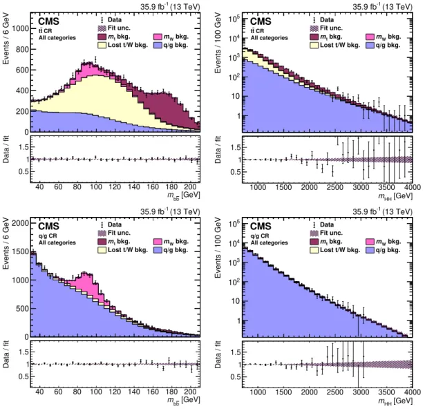
The background models are validated by analyzing the tt CR and q/g CR data samples. For both control regions, background templates are constructed in the same way as for the standard event selection, except that they are made to model the control region selection. The background templates are then fit to the control region data with the same systematic uncertainties that are used in the standard maximum likelihood fit. The result of the

simultaneous fit is shown in figure 2 for both control regions. To improve visualization,

the displayed binning shown in this and subsequent figures is coarser than that used in the maximum likelihood fit. The projections in both mass dimensions are shown for the combination of all event categories. The fit result models the data well, indicating that the shape uncertainties can account sufficiently for potential differences between data and simulation.

7 Systematic uncertainties

Systematic uncertainties are included in the maximum likelihood fit as nuisance param-eters. Nuisance parameters for shape uncertainties are modeled as Gaussian functions,

JHEP10(2019)125

0 200 400 600 800 1000 Events / 6 GeV (13 TeV) -1 35.9 fb CMS CR t t All categories Data Fit unc. bkg. t m m_W bkg. Lost t/W bkg. q/g bkg. 40 60 80 100 120 140 160 180 200 [GeV] b b m 0.5 1 1.5 Data / fit 1 10 2 10 3 10 4 10 5 10 Events / 100 GeV (13 TeV) -1 35.9 fb CMS CR t t All categories Data Fit unc. bkg. t m mW bkg. Lost t/W bkg. q/g bkg. 1000 1500 2000 2500 3000 3500 4000 [GeV] HH m 0.5 1 1.5 Data / fit 0 500 1000 1500 2000 Events / 6 GeV (13 TeV) -1 35.9 fb CMS q/g CR All categories Data Fit unc. bkg. t m m_W bkg. Lost t/W bkg. q/g bkg. 40 60 80 100 120 140 160 180 200 [GeV] b b m 0.5 1 1.5 Data / fit 1 10 2 10 3 10 4 10 5 10 Events / 100 GeV (13 TeV) -1 35.9 fb CMS q/g CR All categories Data Fit unc. bkg. t m m_W bkg. Lost t/W bkg. q/g bkg. 1000 1500 2000 2500 3000 3500 4000 [GeV] HH m 0.5 1 1.5 Data / fit

Figure 2. The fit result compared to data in the tt CR (upper plots) and q/g CR (lower plots), projected in m_bb (left) and mHH (right). Events from all categories are combined. The fit result is the filled histogram, with the different colors indicating different background categories. The background shape uncertainty is shown as the hatched band. The lower panels show the ratio of the data to the fit result.

resolution uncertainties for the signal, the mt background, and the mW background are

evaluated as uncertainties in the mean and standard deviation of the double Crystal Ball

function parameters, respectively. The signal m_HH scale and resolution uncertainties are

handled in the same manner. The other background shape uncertainties are implemented as alternative background templates. Each alternative template is produced by shifting the

nominal background template, bin-by-bin, by a factor that depends on either m_HH or m_bb.

The magnitudes of these factors are subsequently constrained as nuisance parameters. The parameterization of the background uncertainties is motivated by the expectation of possible differences between simulation and data for such aspects as background compo-sition or jet energy scale. Studies of the tt CR and the q/g CR are used to verify that the

JHEP10(2019)125

chosen uncertainties do cover these differences. More complex background models, such as those with more nuisance parameters or higher order shape distortions, are also tested in these control regions. The more complex background models do not lead to better agree-ment between data and the fit result. The fit result does not depend strongly on the initial uncertainty sizes because they function only as loose constraints for the fit. This is verified by inflating all initial background uncertainty sizes by a factor of two and observing that the final result does not change. Therefore, the initial background uncertainty sizes are sufficiently large to easily account for the differences between simulation and data in the control regions.

Shape distortions derived from differences between simulation generator programs, parton showering and simulation programs, and matrix element calculation order were also studied. The uncertainties used in obtaining this result are comparable to or larger than

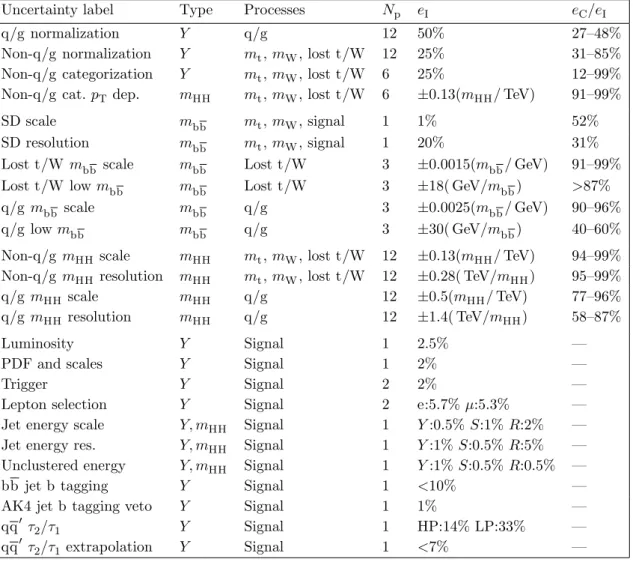
those derived from these differences. Each uncertainty is listed in table 3 with its initial

size. A single uncertainty type can be applied to multiple event categories with independent nuisance parameters per category. The background model includes 98 nuisance parameters, while the signal model includes 13 and shares an additional two with the background model. The description of each uncertainty, including correlations between event categories, is

described in sections 7.1–7.3.

7.1 Background normalization uncertainties

Since the main source of the m_t, m_W, and lost t/W backgrounds is tt production, some

uncertainties are applied by treating the three categories as a single component, referred to collectively as the “non-q/g background”.

The fraction of each of the three categories within the combination is determined from

the overall b tagging efficiency and the bb jet pT distributions. Additional uncertainties

are then assigned to the modeling of their relative composition.

For each event category, the q/g background and the non-q/g background each have a large initial normalization uncertainty that is uncorrelated among categories. The

rel-ative composition of the three tt backgrounds is controlled in two ways. First, the m_W

and lost t/W backgrounds have independent normalization uncertainties per b tagging

category. In both cases, the mt background normalization is varied in an anticorrelated

manner such that the non-q/g background normalization does not change. Second, the

composition is allowed to vary linearly with m_HH to account for bb jet reconstruction

effects that depend on bb jet pT. This is implemented with a mHH shape uncertainty that

only shifts the m_t background spectrum. There is one such independent nuisance

param-eter per b tagging category. Three other nuisance paramparam-eters shift the m_W and lost t/W

backgrounds together.

7.2 Background shape uncertainties

The jet mass scale and resolution after applying the SD algorithm are measured for W bo-son decays merged into single jets in data with tt events, using the known W bobo-son mass. The mass scale and resolution in the simulation are found to agree with the data within

JHEP10(2019)125

Uncertainty label Type Processes N_p e_I e_C/e_I

q/g normalization Y q/g 12 50% 27–48%

Non-q/g normalization Y m_t, m_W, lost t/W 12 25% 31–85%

Non-q/g categorization Y m_t, m_W, lost t/W 6 25% 12–99%

Non-q/g cat. p_T dep. m_HH m_t, m_W, lost t/W 6 ±0.13(mHH/ TeV) 91–99%

SD scale m_bb m_t, m_W, signal 1 1% 52%

SD resolution m_bb m_t, m_W, signal 1 20% 31%

Lost t/W m_bb scale m_bb Lost t/W 3 ±0.0015(m_bb/ GeV) 91–99%

Lost t/W low m_bb m_bb Lost t/W 3 ±18( GeV/m_bb) >87%

q/g m_bb scale m_bb q/g 3 ±0.0025(m_bb/ GeV) 90–96%

q/g low m_bb m_bb q/g 3 ±30( GeV/m_bb) 40–60%

Non-q/g m_HH scale m_HH m_t, m_W, lost t/W 12 ±0.13(m_HH/ TeV) 94–99% Non-q/g m_HH resolution m_HH m_t, m_W, lost t/W 12 ±0.28( TeV/m_HH) 95–99%

q/g m_HH scale m_HH q/g 12 ±0.5(m_HH/ TeV) 77–96%

q/g m_HH resolution m_HH q/g 12 ±1.4( TeV/m_HH) 58–87%

Luminosity Y Signal 1 2.5% —

PDF and scales Y Signal 1 2% —

Trigger Y Signal 2 2% —

Lepton selection Y Signal 2 e:5.7% µ:5.3% —

Jet energy scale Y, m_HH Signal 1 Y :0.5% S:1% R:2% —

Jet energy res. Y, m_HH Signal 1 Y :1% S:0.5% R:5% —

Unclustered energy Y, m_HH Signal 1 Y :1% S:0.5% R:0.5% —

bb jet b tagging Y Signal 1 <10% —

AK4 jet b tagging veto Y Signal 1 1% —

qq0 τ₂/τ₁ Y Signal 1 HP:14% LP:33% —

qq0 τ₂/τ₁extrapolation Y Signal 1 <7% —

Table 3. The systematic uncertainties included in the maximum likelihood fit and how they are applied to each process model. The “type” indicates if the uncertainty affects process yield Y or the shape of the m_bb or mHH distributions. Some uncertainties are applied to multiple event categories with independent nuisance parameters. The number of such parameters, Np, the initial uncertainty size, eI, and the ratios of the constrained size to the initial size, eC/eI, are listed. The ratios are obtained by fitting a model containing only background processes to the data. Uncertainty sizes that vary by event category are listed with category labels. The labels Y , S, and R denote how a single uncertainty affects yield, scale, and resolution, respectively.

uncertainties. These measurements determine the uncertainties in the m_bb scale and

res-olution of the m_t and m_W backgrounds. For the lost t/W and q/g backgrounds, nuisance

parameters are used to account for mismodeling of the simulated energy scale or the low-mass region by morphing the template shapes using a factor that is either proportional to,

or inversely proportional to m_bb, respectively. The m_bb shapes do not vary strongly with

lepton flavor or qq0 τ2/τ1, so a single pair of uncorrelated nuisance parameters is applied

per background and b tagging category.

Mismodeling of the background p_T spectrum could manifest as an incorrect m_HH

JHEP10(2019)125

factors proportional to m_HH. Possible mismodeling of the m_HH resolution is considered

in a similar manner, but with multiplicative factors proportional to m−1_HH. A pair of scale

and resolution uncertainties is assigned to the non-q/g background spectrum for each event

category. An independent set of m_HHuncertainties for the q/g background is also included.

7.3 Signal uncertainties

A 2.5% uncertainty in the integrated luminosity [109] is included as a signal normalization

uncertainty. Signal acceptance uncertainties from the choices of PDF, factorization scale, and renormalization scale are also applied. The scale uncertainties are obtained following

the prescription found in refs. [110,111], and the PDF uncertainty is evaluated using the

NNPDF 3.0 PDF set [73]. Both the simulated trigger selection efficiency and the lepton

selection efficiencies are corrected to match the data efficiencies. The uncertainties in these measurements are included as independent uncertainties in the electron and muon channel signal yields. Uncertainties in the jet energy scale, resolution, and unclustered energy

resolution affect signal acceptance, m_HH scale, and m_HH resolution. The same m_bb scale

and resolution uncertainties that are applied to the m_t and m_W backgrounds are applied

to the signal. In this case, the background and signal uncertainties are 100% correlated. The bb jet b tagging efficiency uncertainty is included as a single nuisance parameter that varies the signal normalization in each b tagging category. The uncertainty depends

on mX, with a maximum size of 10, 4, and 4% for the bT, bM, and bL categories,

re-spectively. The bL category normalization uncertainty is anticorrelated with the other two uncertainties. A normalization uncertainty is assigned to the efficiency for passing

the AK4 jet b tagging veto. The qq0 τ₂/τ₁ selection efficiency is measured in a tt data

sample for W bosons decaying to quarks. The uncertainty in this measurement is included as an uncertainty in the HP and LP category relative yields. An additional extrapolation

uncertainty is applied because the jets in this sample have lower p_T than those in signal

events. The uncertainty depends on m_X, with a maximum value of 7% for m_X = 3.5 TeV.

The LP and HP selection efficiency uncertainties are anticorrelated.

8 Results

The data are interpreted by performing a maximum likelihood fit for a model containing only background processes and one containing both background and signal processes. The background-only fit is found to model the data. We interpret the results as upper limits on the product of the X production cross section and the X → HH branching fraction (σB).

The quality of the fit is quantified with the generalized χ2 goodness-of-fit test using

saturated models [112]. The probability distribution function of the test statistic is obtained

with pseudo-experiments and the observed value is within the central 68% quantile of expected results. The best fit values of the nuisance parameters are consistent with the initial uncertainty ranges.

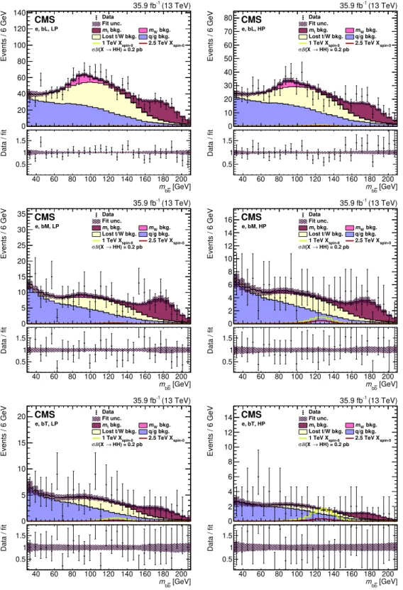
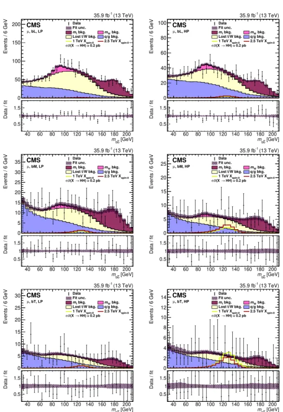
The fit result and the data are projected in m_bb for each event category in figures 3

and4. The shape is modeled well, with each background category contributing to a specific

JHEP10(2019)125

0 20 40 60 80 100 120 140 Events / 6 GeV (13 TeV) -1 35.9 fb CMS e, bL, LP HH) = 0.2 pb → (X Β σ Data Fit unc. bkg. t m mW bkg. Lost t/W bkg. q/g bkg. spin-0

1 TeV X 2.5 TeV X_spin-0

40 60 80 100 120 140 160 180 200 [GeV] b b m 0.5 1 1.5 Data / fit 0 10 20 30 40 50 60 70 80 Events / 6 GeV (13 TeV) -1 35.9 fb CMS e, bL, HP HH) = 0.2 pb → (X Β σ Data Fit unc. bkg. t m mW bkg. Lost t/W bkg. q/g bkg. spin-0

1 TeV X 2.5 TeV X_spin-0

40 60 80 100 120 140 160 180 200 [GeV] b b m 0.5 1 1.5 Data / fit 0 5 10 15 20 25 30 35 Events / 6 GeV (13 TeV) -1 35.9 fb CMS e, bM, LP HH) = 0.2 pb → (X Β σ Data Fit unc. bkg. t m mW bkg. Lost t/W bkg. q/g bkg. spin-0

1 TeV X 2.5 TeV X_spin-0

40 60 80 100 120 140 160 180 200 [GeV] b b m 0.5 1 1.5 Data / fit 0 2 4 6 8 10 12 14 16 Events / 6 GeV (13 TeV) -1 35.9 fb CMS e, bM, HP HH) = 0.2 pb → (X Β σ Data Fit unc. bkg. t m mW bkg. Lost t/W bkg. q/g bkg. spin-0

1 TeV X 2.5 TeV X_spin-0

40 60 80 100 120 140 160 180 200 [GeV] b b m 0.5 1 1.5 Data / fit 0 5 10 15 20 Events / 6 GeV (13 TeV) -1 35.9 fb CMS e, bT, LP HH) = 0.2 pb → (X Β σ Data Fit unc. bkg. t m mW bkg. Lost t/W bkg. q/g bkg. spin-0

1 TeV X 2.5 TeV X_spin-0

40 60 80 100 120 140 160 180 200 [GeV] b b m 0.5 1 1.5 Data / fit 0 2 4 6 8 10 12 14 Events / 6 GeV (13 TeV) -1 35.9 fb CMS e, bT, HP HH) = 0.2 pb → (X Β σ Data Fit unc. bkg. t m mW bkg. Lost t/W bkg. q/g bkg. spin-0

1 TeV X 2.5 TeV X_spin-0

40 60 80 100 120 140 160 180 200 [GeV] b b m 0.5 1 1.5 Data / fit

Figure 3. The fit result compared to data projected in m_bb for the electron event categories. The fit result is the filled histogram, with the different colors indicating different background categories. The background shape uncertainty is shown as the hatched band. Example spin-0 signal distribu-tions for mX of 1 and 2.5 TeV are shown as solid lines, with the product of the cross section and branching fraction to two Higgs bosons set to 0.2 pb. The lower panels show the ratio of the data to the fit result.

JHEP10(2019)125

0 50 100 150 200 Events / 6 GeV (13 TeV) -1 35.9 fb CMS , bL, LP µ HH) = 0.2 pb → (X Β σ Data Fit unc. bkg. t m mW bkg. Lost t/W bkg. q/g bkg. spin-0

1 TeV X 2.5 TeV X_spin-0

40 60 80 100 120 140 160 180 200 [GeV] b b m 0.5 1 1.5 Data / fit 0 20 40 60 80 100 Events / 6 GeV (13 TeV) -1 35.9 fb CMS , bL, HP µ HH) = 0.2 pb → (X Β σ Data Fit unc. bkg. t m mW bkg. Lost t/W bkg. q/g bkg. spin-0

1 TeV X 2.5 TeV X_spin-0

40 60 80 100 120 140 160 180 200 [GeV] b b m 0.5 1 1.5 Data / fit 0 5 10 15 20 25 30 35 Events / 6 GeV (13 TeV) -1 35.9 fb CMS , bM, LP µ HH) = 0.2 pb → (X Β σ Data Fit unc. bkg. t m mW bkg. Lost t/W bkg. q/g bkg. spin-0

1 TeV X 2.5 TeV X_spin-0

40 60 80 100 120 140 160 180 200 [GeV] b b m 0.5 1 1.5 Data / fit 0 5 10 15 20 25 Events / 6 GeV (13 TeV) -1 35.9 fb CMS , bM, HP µ HH) = 0.2 pb → (X Β σ Data Fit unc. bkg. t m mW bkg. Lost t/W bkg. q/g bkg. spin-0

1 TeV X 2.5 TeV X_spin-0

40 60 80 100 120 140 160 180 200 [GeV] b b m 0.5 1 1.5 Data / fit 0 5 10 15 20 25 30 Events / 6 GeV (13 TeV) -1 35.9 fb CMS , bT, LP µ HH) = 0.2 pb → (X Β σ Data Fit unc. bkg. t m mW bkg. Lost t/W bkg. q/g bkg. spin-0

1 TeV X 2.5 TeV X_spin-0

40 60 80 100 120 140 160 180 200 [GeV] b b m 0.5 1 1.5 Data / fit 0 2 4 6 8 10 12 14 Events / 6 GeV (13 TeV) -1 35.9 fb CMS , bT, HP µ HH) = 0.2 pb → (X Β σ Data Fit unc. bkg. t m mW bkg. Lost t/W bkg. q/g bkg. spin-0

1 TeV X 2.5 TeV X_spin-0

40 60 80 100 120 140 160 180 200 [GeV] b b m 0.5 1 1.5 Data / fit

Figure 4. The fit result compared to data projected in m_bb for the muon event categories. The fit result is the filled histogram, with the different colors indicating different background categories. The background shape uncertainty is shown as the hatched band. Example spin-0 signal distribu-tions for mX of 1 and 2.5 TeV are shown as solid lines, with the product of the cross section and branching fraction to two Higgs bosons set to 0.2 pb. The lower panels show the ratio of the data to the fit result.

JHEP10(2019)125

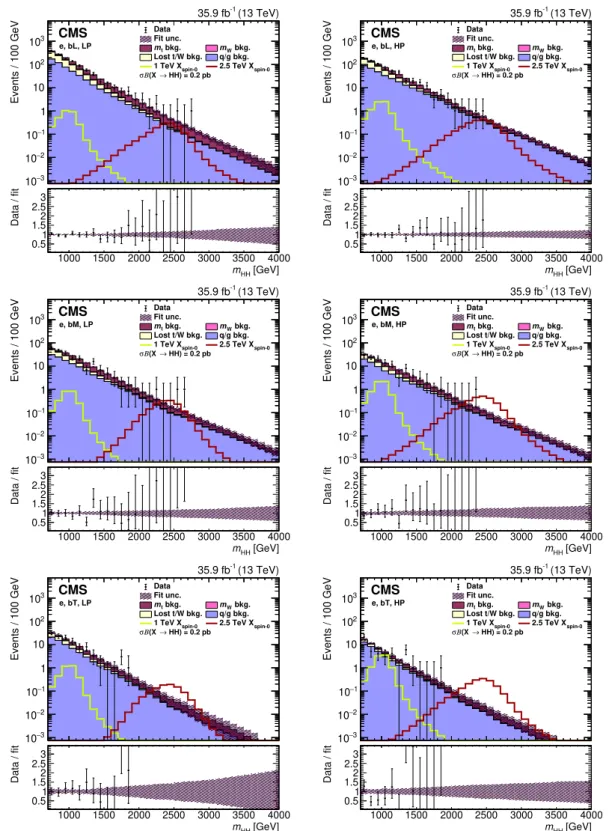
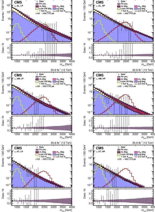
top quark decays are correctly modeled by the fit. Similarly, the projection in m_HH for

each event category is shown in figures 5 and 6. Good agreement is found for the entire

m_HH mass range.

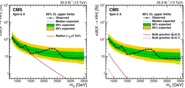
The 95% confidence level (CL) upper limits are shown in figure 7 for varying mX and

both the spin-0 and spin-2 boson scenarios. The limits are evaluated using the

asymp-totic approximation [113] of the CL_s method [114, 115]. The observed exclusion limit

is consistent with the expected limit; the most significant deviation between the two is

about 1.5 standard deviations at m_X ≈ 2.3 TeV. The sources of the discrepancy are small

excesses in data at high m_HH for the µ, bM, LP and µ, bL, HP event categories. The

mX = 0.8 TeV spin-0 signal is excluded for σB > 123 fb, with the exclusion limit

strength-ening to σB > 8.3 fb for m_X = 3.5 TeV signal. The higher signal acceptance for spin-2

signal results in stronger constraints on σB: >103 fb for mX = 0.8 TeV signal and >7.8 fb

for m_X = 3.5 TeV signal. This search yields the best limits in this decay channel for

X → HH production. It has similar sensitivity to resonances with m_X≈ 1 TeV to searches

performed in other channels [50, 56]. This search is less sensitive to mX & 1.5 TeV

res-onances because of the degradation of the lepton selection efficiency for events with very large boost.

Predicted radion and bulk graviton cross sections [116] are also shown in figure7in the

context of Randall-Sundrum models that allow the SM fields to propagate though the extra

dimension. Typical model parameters are chosen as proposed in ref. [117]. For radions,

a branching fraction of 25% to HH and an ultraviolet cutoff Λ_R = 3 TeV are assumed.

A 10% branching fraction is assumed for bulk gravitons, which occurs in scenarios that

include significant coupling between the bulk graviton and top quarks. Bulk graviton

production cross sections depend on the dimensionless quantity ek =√8πk/M_Pl, where k is

the curvature of the extra dimension and M_Pl is the Planck mass. For this interpretation,

we choose ek = 0.1 and 0.3. For these particular signal parameters the radion and bulk

graviton decay widths are larger than the 1 MeV width chosen for signal sample generation, but smaller than the detector resolution.

9 Summary

A search has been presented for new particles decaying to a pair of Higgs bosons (H) where one decays into a bottom quark pair (bb ) and the other into two W bosons that subsequently decay into a lepton, a neutrino, and a quark pair. The large Lorentz boost of the Higgs bosons leads to the distinct experimental signature of one large-radius jet with substructure consistent with the decay H → bb and a second large-radius jet with a

nearby isolated lepton consistent with the decay H → WW∗. This search uses a sample

of proton-proton collisions collected at √s = 13 TeV by the CMS detector, corresponding

to an integrated luminosity of 35.9 fb−1. The primary standard model background, top

quark pair production, is suppressed by reconstructing the HH decay chain and applying mass constraints. The signal and background yields are estimated by a two-dimensional template fit in the plane of the bb jet mass and the HH resonance mass. The templates are validated in a variety of data control regions and are shown to model the data well. The

JHEP10(2019)125

3 − 10 2 − 10 1 − 10 1 10 2 10 3 10 Events / 100 GeV (13 TeV) -1 35.9 fb CMS e, bL, LP HH) = 0.2 pb → (X Β σ Data Fit unc. bkg. t m mW bkg. Lost t/W bkg. q/g bkg. spin-0

1 TeV X 2.5 TeV Xspin-0

1000 1500 2000 2500 3000 3500 4000 [GeV] HH m 0.51 1.52 2.53 Data / fit 3 − 10 2 − 10 1 − 10 1 10 2 10 3 10 Events / 100 GeV (13 TeV) -1 35.9 fb CMS e, bL, HP HH) = 0.2 pb → (X Β σ Data Fit unc. bkg. t m mW bkg. Lost t/W bkg. q/g bkg. spin-0

1 TeV X 2.5 TeV Xspin-0

1000 1500 2000 2500 3000 3500 4000 [GeV] HH m 0.51 1.52 2.53 Data / fit 3 − 10 2 − 10 1 − 10 1 10 2 10 3 10 Events / 100 GeV (13 TeV) -1 35.9 fb CMS e, bM, LP HH) = 0.2 pb → (X Β σ Data Fit unc. bkg. t m mW bkg. Lost t/W bkg. q/g bkg. spin-0

1 TeV X 2.5 TeV X_spin-0

1000 1500 2000 2500 3000 3500 4000 [GeV] HH m 0.51 1.52 2.53 Data / fit 3 − 10 2 − 10 1 − 10 1 10 2 10 3 10 Events / 100 GeV (13 TeV) -1 35.9 fb CMS e, bM, HP HH) = 0.2 pb → (X Β σ Data Fit unc. bkg. t m mW bkg. Lost t/W bkg. q/g bkg. spin-0

1 TeV X 2.5 TeV X_spin-0

1000 1500 2000 2500 3000 3500 4000 [GeV] HH m 0.51 1.52 2.53 Data / fit 3 − 10 2 − 10 1 − 10 1 10 2 10 3 10 Events / 100 GeV (13 TeV) -1 35.9 fb CMS e, bT, LP HH) = 0.2 pb → (X Β σ Data Fit unc. bkg. t m mW bkg. Lost t/W bkg. q/g bkg. spin-0

1 TeV X 2.5 TeV X_spin-0

1000 1500 2000 2500 3000 3500 4000 [GeV] HH m 0.51 1.52 2.53 Data / fit 3 − 10 2 − 10 1 − 10 1 10 2 10 3 10 Events / 100 GeV (13 TeV) -1 35.9 fb CMS e, bT, HP HH) = 0.2 pb → (X Β σ Data Fit unc. bkg. t m mW bkg. Lost t/W bkg. q/g bkg. spin-0

1 TeV X 2.5 TeV X_spin-0

1000 1500 2000 2500 3000 3500 4000 [GeV] HH m 0.51 1.52 2.53 Data / fit

Figure 5. The fit result compared to data projected in mHH for the electron event categories. The fit result is the filled histogram, with the different colors indicating different background categories. The background shape uncertainty is shown as the hatched band. Example spin-0 signal distribu-tions for mX of 1 and 2.5 TeV are shown as solid lines, with the product of the cross section and branching fraction to two Higgs bosons set to 0.2 pb. The lower panels show the ratio of the data to the fit result.