Signal recovery from partial fractional fourier transform information

(1)

SIGNAL RECOVERY FROM PARTIAL FRACTIONAL FOURIER TRANSFORM

INFORMATION

A .

Enis Getin', Hakan Ozaktas2, Haldun

M. Ozaktas'

Bilkent University, Department

of

Electrical and Electronics Engineering, Bilkent

Ankara, 06800, Turkey.

Eastern Mediterranean University Department

of

Industrial Engineering Famagusta,

TRNC.

ABSTRACT

The fractional Fourier transform has found many applications in signal and image processing and optics. An iterative algorithm for signal recovery from partial fractional Fourier transform information is presented. The signal recovery algorithm is constructed by using the method of projections onto convex sets and convergence of the algorithm is assured.

1. INTRODUCTION

The fractional Fourier transform is widely used in optics and found applications in signal and image processing [ 13- [SI. The p-th order fractional Fourier transform operation corresponds to the p-th power of the ordinary Fourier transform operation. The zeroth-order fractional Fourier transform of a function is the function itself and the first-order transform is equal to the ordinary Fourier transform. In optics, it is well-known that Fourier Transform of an object corresponds to the image of the object at the focal point of the lens, and fractional Fourier Transform describes the image of the object in the near field of the lens for 0 < p

<

1. In this paper, an iterative algorithm for signal recovery from partial fractional Fourier transform information is developed by making alternating projections onto sets representing measurements in fractional Fourier domains. In other words, the image of the object may be reconstructed from partial near field measurements. The reconstruction algorithm is globally convergent and it is based on the method of projections onto convex sets (POCS), a classical numerical technique [6]. The convergence of t h s algorithm can be proved easily in both continuous and discrete Fractional Fourier Transform domains because both partial fractional Fourier information in a band or in a location correspond to closed and convex sets in L2 or C2, respectively. Other closed and convex sets that may be used in the reconstruction algorithm include sets representing bounded energy, non-negativity constraint and finite-support information in

time domain.

In the next section, basic concepts of fractional Fourier Transform is reviewed. In Section 111, the signal recovery algorithm is presented, and simulation examples are presented in the last section.

2. FRACTIONAL FOURIER TRANSFORM

In this section, Fractional Fourier Transform is briefly reviewed and the signal recovery problem is presented. For a thorough discussion of the Fractional Fourier Transform and its properties the reader is referred to [ 11-[SI.

Let us denote the pth order fractional Fourier transform operator as FP. When p = 1 we have the ordinary Fourier transform operator

F.

Fractional Fourier transform is defined by the standard eigenvalue methods for finding a function

G(31)

of a linear operator 3t. Hermite-Gaussian functions are the eigenfunctions of the regular Fourier transform:

F?,bn(u)

= exp(-in.rr/2)?,bn(u), where ?,bn(u),

n = 0,1,2,

. . .

are the set of Hermite-Gaussian functions: 2 1 / 4 ( Z n n ! ) - 1 / 2 H n ( d % u ) exp(-.rru2) and & ( U ) are the

standard Hermite polynomials. The fractional Fourier transform is defined in terms of the eigenvalue equation FP?,bn(u) = [exp(-in.rr/Z)]P$~~(u) where the fractional pth power satisfies [ e x p ( - i n ~ / 2 ) ] P = e x p ( - i p n ~ / 2 ) . An analytic expression for the fractional Fourier transform of an arbitrary square-integrable function z ( t ) is obtained by expanding it in terms of the complete orthonormal set of functions ?,bn(u) and then applying the above eigenvalue equation to each term of the expansion. It is shown in [3] that the pth order fractional Fourier transform z p ( u ) E

F P z ( u ) is given by

-2 csc(pn/2)ut

+

cot(p7r/Z)t2)]dt (1) The zeroth-order fractional Fourier transform of a function is the function itself and the fist-order transform is equal to

0-7803-8379-6/04/$20.00 02004 IEEE.

(2)

the ordinary Fourier transform. Positive and negative inte- ger values of p simply correspond to repeated application of the ordinary forward and inverse Fourier transforms respectively. The fractional Fourier transform operator satisfies index additivity: 3 P 2 3 P 1 = 3 P 2 + P 1 . The operator 3 P is periodic in p with period 4 since

FT2

equals the parity operator which maps

z ( t )

to z(-t) and

F4

equals the identity operator.

The pth order discrete fractional Fourier transform X, of an N x 1 vector x is defined as X, = Fax, where

X"

is the N x

N

discrete fractional Fourier transform matrix [ 5 ] , which is essentially the pth power of the ordinary discrete Fourier transform matrix X. Let the discrete-time vector x contains the samples of the continuous time signal

z ( t ) ,

and if N is chosen equal to or greater than the space-bandwidth product of the signal

z ( t ) ,

then the discrete fractional transform approximates the continuous fractional transform in the same way as the ordinary discrete transform approximates the ordinary continuous transform.

The signal recovery problem is the reconstruction of

z ( t )

from

z P ( u ) ,

U E

U

where

U

is a subset of

R.

The set

U may consist of union of some bands in the p-th fractional Fourier domain. It may also contain or consist of iso- lated discrete points representing measurements of z p ( u ) at

ui

,

i = 1

,

2, .

.

,

I As in the case of signal recovery from partial Fourier Transform information, the reconstruction problem is very noise sensitive, if U represents a narrow band in the p-th fractional Fourier transform domain. In addition to recordings in the p-th fractional domain, measurements can be available in the q-th fractional domain and this information can be used for signal recovery as well.

3. ITERATIVE SIGNAL RECOVERY ALGORITHM This section presents the signal recovery algorithm which is devised by using the method of projections onto convex sets (POCS) [6] that has been successfully used in many signal recovery and restoration problems [SI-[lo]. The key idea is to obtain a solution which is consistent with all the available information. In this method the set of all possible signals is assumed to constitute a Hilbert space with an associated norm in which the prior information about the desired signal can be represented in terms of convex sets. In this paper, the Hilbert space is L2 or l2 with Euclidian norm for continuos time and discrete-time signals, respectively. Let us suppose that the information about the desired signal is represented by M sets, C,,

m

= 1 , 2 ,

...,

M . Since the desired signal satisfies all of the constraints it must be in the intersection set

CO

= n,",,C,. Any member of the set

CO

is called a feasible solution [lo]. If all of the sets C, are closed and convex then a feasible solution can be found by making successive orthogonal projections onto sets, C,. Let P,

be the orthogonal projection operator onto the set

C,.

The iterates defined by the following equation

converge to a member of the set

CO,

regardless of the ini- tial signal yo. The number of convex sets can be infinite. The rate of convergence can be improved by using non- orthogonal projections as well. The underlying mathemati- cal concepts can be found in [6],[7].

We define the set C1 in L2 as the set of signals whose fractional Fourier Transform are equal to z p ( u ) in the band U E U in the p-th fractional domain. This set is convex because the integral operator in (1) is a linear operator. The proof of closure can be established as in []. If data is also avalible in the q-th fractional domain another set C2 can be defined in a similar manner. If the signal is

a finite extent signal then this information can be modelled as a closed and convex set as in other regular signal reconstruction problems. Actually, any time-domain information about the original signal including

z ( t ) =

0 in a bounded or unbounded window in time domain and non-negativity information belongs to the above class of sets in fractional Fourier domain as time-domain corresponds to the case of p = 0. Equation (1) simply becomes the identity operator for the fraction p = 0.

Partial information in the discrete fractional Fourier domain can be represented as convex sets in l2 in discrete-time domain as well.

Another convex set which can be used in the signal recovery algorithm is the bounded energy set, C, which is the set of sequences whose energy is bounded by eo, i.e.,

(3) This set provides robustness against noise, if eo is known or

some idea about eo is available.

Other convex sets describing partial fractional Fourier domain information can be defined as in [].

The key operation of the method of POCS is the orthogonal projection onto a convex set. Projection operations onto the sets C1, C2,

...,

CK

are straightforward to implement. Let

dk)

( t )

be the Ic-th iterate of the iterative recovery process. Let zL"(u) be fractional Fourier transform of

dk)

in the p-th domain. The projection operator replaces the fractional Fourier transform values of

zp)

( U ) in the band U

zF+1)(u) = z p ( u ) U E U , (4)

and retains the rest of the data outside the band U :

(3)

Projection onto the set C, is described in [SI. It simply consists of scaling the signal x(t) such that the energy of the scaled signal is E , . Projection onto the non-negativity set C, is carried out by simply forcing the negative values of

x ( t ) to zero.

Let us describe the signal recovery algorithm from partial fractional Fourier transform information. The algorithm starts with an arbitrary initial estimate y(0) E L 2 .

The initial estimate yo is successively projected onto the sets

C,,

m = 1 , 2 ,

...,

M , representing the partial fractional Fourier domain information in fractional domains

p,, m = 1,2,

...,

M by using Equations (3) and (4). The order of projections is immaterial. In this manner the first iteration cycle is completed and the K-th iterate y ( K ) is obtained. If the energy (non-negativity) information is available then the current iterate is also projected also onto the

set C, (C,). This iterative procedure is repeated until a sat-

isfactory level of error difference in successive iterations is obtained.

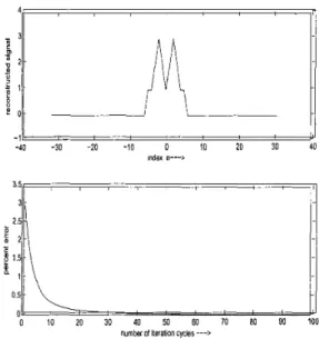
sets used in the reconstruction process. In Fig. 2(a), the reconstructed signal is shown, and percent error versus the number of iteration cycles is shown in Fig. 2(b).

In all the examples tried we have observed the consistent behavior of the algorithm.

If the fractional Fourier domain data is available only in a narrow band then the reconstruction process can be noise sensitive as in regular signal reconstruction from partial Fourier domain data problem.

5. CONCLUSION:

This paper presents an iterative algorithm for signal recovery from partial fractional Fourier transform domain information. The signal reconstruction algorithm is developed by using the method of projection onto convex sets. Con- vergence is assured regardless of the initial estimate.

The signal recovery technique can be easily extended to multi-dimensional signal recovery problems as well. 4. SIMULATION EXAMPLES:

6. REFERENCES In many practical problems, some measurements

xp(u)

at

ui,

i = 1 , 2 ,

...,

I,, .,(U)

at

ul,

2 = 1 , 2 ,

..., I,

etc, and the finite-support information x ( t ) = 0, f o r t

<

t o ,

and

t

>

tl

are available, and the fractional Fourier Transform integral (1) is numerically approximated. If the fractional Fourier data is available in a uniform grid then discrete fractional Fourier transform can be used in the recovery algorithm.

Consider the following simulation example. It is assumed that the fractional Fourier domain data is available in a uniform grid. It is assumed that N=64 point discrete fractional Fourier transform vector Xo.5 of the desired discrete-time signal

x

= { 1 , 2 , 3 , 2 , 1 , 1 , 1 , 2 , 3 , 2 , 1 , 0 , 0 , ...} is available for X , . , [ k ] ,

/ k

= 16,12,

...,

50. Available time domain information about the signal is the following: x[n] = 0 for

n

<

0 and n

>

20. The percent error versus the number of iteration cycles is shown in Figure 1. Percent restoration error is defined as follows: 100 x 11yk -

XI

12//1

1x1

l2

where yh is the k-th iterate. Clearly, the original signal can be recovered with negligible error. Iterates converge after 10 iteration cycles.

In the second experiment, fractional Fourier domain information about the original signal is the same as above but available time domain information about the signal is that the signal is causal and non-negative. In other words, it is known that s[n]

=

0 for

n

<

0 and

x[n]

2

0 for all

n.

In this case, a signal close to the original signal is obtained. It turns out that the prior information about the original signal is not enough to uniqely reconstruct it. But iterates converge to a member of the set

C,

which is the intersection of all the

H. M. Ozaktas, B. Barshan, D. Mendlovic, and L. Onural. Convolution, filtering, and multiplexing in fractional Fourier domains and their relation to chirp and wavelet transforms. J Opt SOC Am A, 1 1 :547-559, 1994.

L. B. Almeida. The fractional Fourier transform and time-frequency representations. IEEE Trans Signal Processing, 42:3084-309 1, 1994.

H. M. Ozaktas, Z. Zalevsky, and M. A. Kutay. The Fractional Fourier Transform with Applications in

Optics and Signal Processing. Wiley, New York, 200 1. H. M. Ozaktas and D. Mendlovic. Fractional Fourier optics. J Opt Soc Am A, 12:743-751,1995.

C.

Candan, M. A. Kutay, and H. M. Ozaktas. The discrete fractional Fourier transform. IEEE Trans Signal

Processing, 48: 1329-1337,2000.

D.C. Youla and H. Webb ,‘Image restoration by the method of Convex Projections, Part 1-Theory’, IEEE Trans. on Medical Imaging, vol. MI-1, no.2, pp.81-94, Oct. 1982.

P. L. Combettes, “The foundations of set theoretic es- timation,” em Proceedings of the IEEE, vol. 81, no. 2, pp. 182-208, February 1993.

(4)

1Y , I , I /

-40 -30 -20 -10 0 10 20 30 40

I , . .. , , : ,... I i

0 500 1000 1500 2000 2500 30W 3500 4000 4500 50’

number of iteration cvdes -->

Figure 1: (a) Reconstructed signal (top), and (b) percent error versus the number of iteration cycles (bottom) in Ex- ample 1.

[8] M. I. Sezan and H. Stark, ‘Image restoration by the method of Convex Projections, Part-2: Applications and Numerical Results’, IEEE Trans. on Medical

Imaging, vol. MI-1, no.2, pp.95-101,Oct. 1982. [9] H. J. Trussell and M. R. Civanlar, ‘The Feasible

solution in signal restoration,’ IEEE Trans. Acoust., Speech, and Signal Proc., vol. 32, pp. 201-212, 1984. [lo] A. E. Cetin and R. Ansari, ‘ A convolution based framework for signal recovery,’ Journal of Optical So- ciety o f h z e r i c a d , pp. 1193-1200, vo1.5, Aug. 1988.

I

-40 -30 -20 -10 0 10 20 30 40

index n--->

3.5

/ / I

Figure 2: (a) Reconstructed signal (top), and (b) percent error versus the number of iteration cycles (bottom) in Ex- ample 2.