Full Terms & Conditions of access and use can be found at
http://www.tandfonline.com/action/journalInformation?journalCode=tprs20
Download by: [Bilkent University] Date: 13 November 2017, At: 03:01
ISSN: 0020-7543 (Print) 1366-588X (Online) Journal homepage: http://www.tandfonline.com/loi/tprs20
Simulation metamodelling with neural networks:
An experimental investigation
Ihsan Sabuncuoglu & Souheyl Touhami
To cite this article: Ihsan Sabuncuoglu & Souheyl Touhami (2002) Simulation metamodelling
with neural networks: An experimental investigation, International Journal of Production Research, 40:11, 2483-2505, DOI: 10.1080/00207540210135596
To link to this article: http://dx.doi.org/10.1080/00207540210135596
Published online: 14 Nov 2010.
Submit your article to this journal
Article views: 73
View related articles
Simulation metamodelling with neural networks: an experimental
investigation
IHSAN SABUNCUOGLUy* and SOUHEYL TOUHAMIz
Arti®cial neural networks are often proposed as an alternative approach for formalizing various quantitative and qualitative aspects of complex systems. This paper examines the robustness of using neural networks as a simulation metamodel to estimate manufacturing system performances. Simulation models of a job shop system are developed for various con®gurations to train neural network metamodels. Extensive computational tests are carried out with the proposed models at various factor levels (study horizon, system load, initial system status, stochasticity, system size and error assessment methods) to see the metamodel accuracy. The results indicate that simulation metamodels with neural networks can be e ectively used to estimate the system performances.
1. Introduction
Simulation has been widely accepted by the scienti®c community and practi-tioners as a ¯exible tool in modelling and analysis of complex systems. It reduces the cost, time and risks associated with the implementations of new designs. However, due to its lengthy computational requirements and the trail-and-error nature of the development process, simulation may not be always the ®rst preferred tool in solving real-life problems. This issue is particularly important for problems where the solution space is very large and when the time available for decision-making is too limited for extensive analysis to be performed (i.e. on-line applica-tions). Harmonosky and Robohn (1995) stated that CPU requirements appeared to be a major obstacle for the on-line applications of simulation. Time considerations are still an important issue, even with the o -line use of simulation due to the increasing complexity of the modern production systems. In this paper, it is argued that the use of simulation metamodels may help alleviate these problems.
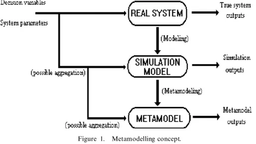
A simulation metamodel is a simpler model of the real system. The simulation model is an abstraction of the real system in which a selected subset of inputs is considered. The e ect of the excluded inputs is represented in the model in the form of the randomness to which the system is subject. As illustrated in ®gure 1, a meta-model is a further abstraction of the simulation meta-model. Simulation is used to gen-erate data sets, which in turn are used to build the metamodel. A simulation metamodel with neural networks is a neural network whose training is provided by a simulation model. In general, a metamodel takes a fewer number of inputs
International Journal of Production Research ISSN 0020±7543 print/ISSN 1366±588X online # 2002 Taylor & Francis Ltd http://www.tandf.co.uk/journals
DOI: 10.1080/00207540210135596 Revision received November 2001.
{ Bilkent University, Department of Industrial Engineering, Faculty of Engineering, 06533 Ankara, Turkey.
{ Concordia University, Department of Decision Sciences &MIS, John Molson School of Business, 1455 de Maisonneuve Blvd. W. GM209-11, Montreal, QueÂbec, H3G 1M8, Canada.
* To whom correspondence should be addressed. e-mail: [email protected]
and is usually simpler than the simulation model. These savings result in lower running times, but at the expense of a reduction of the accuracy of the metamodel with respect to the original system.
Research in metamodelling is maturing. Since the late 1980s, the literature reveals a resurgence of interest in metamodelling in general and speci®cally in neural net-work-based metamodels. In this study, we develop and test simulation metamodels with back propagation arti®cial neural networks for the purpose of estimating system performance measures in job-shop scheduling environments. Extensive com-putational experiments are also carried out to identify the critical factors that a ect the estimation process and accuracy of metamodels. The results provide important insights into the e ective use of the simulation metamodels with neural networks.
The paper is organized as follows. Section 2 gives the research background and motivation behind the study. The details of the proposed study and the experimental settings are given in Section 3. The results are presented in Section 4, where the performances of the metamodels are also discussed. Concluding remarks and future research directions are given in Section 5.
2. Research Background
The metamodels are used to reduce the computer costs (memory and time) of simulation while making use of its potential of estimating performance of complex systems. Blanning (1975) is probably among the ®rst scientists to propose the use of metamodels to alleviate the problems of simulation. The application of metamodels for manufacturing systems’ management has increase since then. As pointed out by Yu and Popplewell (1994), the increases in publications for metamodelling of manu-facturing systems indicates that the technique is of value in manumanu-facturing systems’ design and analysis. The related bibliography of metamodeling is as follows.
Friedman and Pressman (1988) explored the advantages of metamodelling. These included model simpli®cation, enhanced exploration and interpretation of the model, generalization to other models of the same type, sensitivity analysis, answer-ing inverse questions and a better understandanswer-ing of the studied system and the
Figure 1. Metamodelling concept.
interrelationships of system variables. Barton (1992) provided a review on general-purpose mathematical approximations to simulation input±output functions. According to him, one of the major issues in the design of the mathematical approx-imation is the choice of a functional form for the output function. The metamodel-ling candidate approaches include Taguchi models, generalized linear models, radial basis functions, Kernel methods, spatial correlation models, frequency domain approximations and robust regression methods. Barton concluded that while some approaches cannot provide a global ®t to smooth response functions of arbitrary shape, the others are computationall y intensive and in some cases estimation prob-lems are numerically ill-conditioned. Despite these potential drawbacks, these approaches produced satisfactory results. See McHaney and Douglas (1990) and Watson et al. (1994) for sample success stories with regression-based metamodels. A methodology for ®tting and validating regression-based metamodels were dis-cussed in detail by Kleijnen and Sargent (2000). There are also metamodels devel-oped by using rule-based expert systems (Pierreval 1995).
The use of neural networks is another approach for metamodelling that has recently emerged. This study aims at investigating the robustness of neural net-work-based simulation metamodels. Speci®cally, it employs back propagation neural networks that belong to the supervised learning category. The major distin-guishing feature of back propagatio n neural networks is learning the underlying mappings between the input and output variables from examples (Dayho 1990). In a traditional computer program, the programmer speci®es every step in advance. The neural network, in contrast, would by itself build the mapping describing the input±output relationship and no programming is required. This is achieved through the learning process. Another important feature of neural networks is generalization. Although learning is based only on a limited set of examples, when it comes to applying the neural network model, the network should be able to extend its knowl-edge to outside this set of examples.
Neural networks have a wide range of applications . Zhang and Huang (1995) discussed the applications of neural networks in general. Burke and Ignozio (1992) reviewed the application of neural networks in operations research. Sabuncuoglu (1998) presented the theory and applications of neural networks in production sched-uling. It appears that the interest in neural networks that mainly started from 1987 corresponds to the same time for which a resurgence of interest was noted for the use of metamodelling in manufacturing environments.
Even though neural networks have many success stories, one must recognize that metamodelling with neural networks has some shortcomings (Madey et al. 1990). First, constructing a neural network is time consuming since the process requires generating a training set, and empirically selecting an appropriate architecture. Second, the accuracy of the network outputs depends on the regularity of the behav-iour of the system under study (by regularity, we mean that the system is subject to the same set of exogenous and uncontrollable factors). This implies that the time horizon of the study must be carefully selected. Third, the validity of the results also depends on the degree of aggregation selected for the input data. Aggregation of data is needed to reduce the size of the neural network and the e ort required at generating the examples. This would have a negative impact on the precision of the neural network results. The disadvantage s mentioned so far are common to most metamodelling techniques. Another more speci®c problem related to metamodelling with neural networks is the di culty of making interpretations and analysis of the
input±output relationship. As mentioned above, the neural network generates its own rules but does not provide them explicitly to the user. To get an insight into the input±output relationship, one needs to analyse the weights of the connections between the processing units. This is not an easy task, and it is time consuming. Thus, providing a formal method to analyse the neural network may strengthen its value as a metamodelling approach. A brief summary of neural network applications to metamodelling is as follows.
Chryssolouris et al. (1990) used a neural network metamodel to reduce the com-putational e orts required in the long trial process associated with using simulation alone for the design of a manufacturin g system. Chryssolouris et al. (1991) deter-mined the parameters of the operational policy required to achieve some given levels system performances for their neural network metamodel. Mollaghasem i (1998) developed a neural network-based metamodel for the system design problem. Hurrion (1992) employed a neural network to estimate con®dence intervals for the performance of an inventory depot. Hurrion (1997) combined the neural metamodel with simulation to speed up the search process in simulation. In a recent study, Hurrion (1998) proposed the visual interactive metasimulation using neural network. Pierreval (1993) employed neural networks to rank dispatching rules in a stoch-astic ¯ow shop. In the follow-up study, Pierreval (1996) investigated the ability of neural networks to estimate mean machine utilization of a deterministic small-sized problem. Philipoom et al. (1994) employed the neural networks as a simulation metamodel to assign due dates for jobs based on system characteristics and system status when jobs enter system. Badiru and Sieger (1998) proposed neural networks as a simulation metamodel in economic analysis of risky projects. Kilmer et al. (1999) use supervised neural networks as a metamodelling technique for discrete-event, stochastic simulation. The authors translated an (s; S) inventory simulation into a metamodel and estimated the expected total and its variance. They formed con-®dence intervals from both metamodels and the simulation model. The results indi-cate that the neural network metamodel is quite competitive in accuracy when compared with the simulation itself. They also showed that one neural network metamodels are trained, they can operate nearly in real-time. Huang et al. (1999) employed neural networks for the performance prediction system to help in identify-ing abnormalities in the system. Finally, Aussem and Hill (2000) proposed the use of neural networks as a metamodelling technique to reduce the computational burden of stochastic simulations. The proposed metamodel was successfully used to predict the propagation of the green alga in the Mediterranean.
To the best of our knowledge, there is not much work reported to compare the di erent metamodelling approaches. Among a few studies, Philipoom et al. (1994) compared the regression models and neural network models on the task of selected due date assignment rules. Their results showed a great success for neural networks compared with the regression models. Hurrion and Birgil (1999) compared two forms of experimental design methods (full factorial designs and random designs) used for the development of regression and neural network simulation metamodels. Their results showed that the neural network metamodel outperform conventional regression metamodels, especially when data sets based on randomized simulation experimental designs are used to produce the metamodels rather than data sets from similar-sized full-factorial experimental designs.
Raaymakers and Weijters (2000) used neural networks to estimate makespan in batch-processing industries. The results of their simulation experiments indicated
that the estimation quality of the neural network models is signi®cantly better than the quality of regression models. There are also opposite results in the literature. For example, Fishwick (1989) found that a neural network model performs poorly when compared with a linear regression model and a surface response model applied to a ballistic system when measuring the horizontal distance covered by a projectile. We believe that both neural networks and regression models are good scienti®c tools in dealing with estimation problems. They have their own di erent characteristics that should be studied further in various problem domains. There even may be areas in which both can be used in a complementary fashion to enhance the solution quality. This requires further investigation by researchers. Unfortunately, this is not within the scope of this paper.
In all the papers discussed above, neural network-based metamodels achieve reasonably good results. Several of the experiments report a percentage error of µ 6. In these studies, the researchers showed that neural networks are very promising tools for predicting system measures. However, all these case studies deal with systems of reduced complexities or ones of a deterministic nature and do not allow us to generalize on the estimation capabilities of neural networks. In this study, in fact, we investigate how such factors a ect the precision of the neural metamodels. The objective of this experimental investigation is to determine system characteristics for which the use of neural metamodels can be expected to produce an acceptable level of accuracy.
3. Proposed study
This study considers a job shop manufacturing system. Simulation models and neural metamodels are developed for the purpose of estimating system performance measures under various system con®gurations. Three sets of experiments are con-sidered. The ®rst is conducted to estimate the mean machine utilization for a system in steady-state . This is referred to as estimating long-term mean machine utilization. The second set of experiments is similar to the ®rst, except that long-term mean job tardiness is estimated. In these two sets of experiments, the following factors are examined.
. System complexity: simple versus complex.
. Stochasticity: deterministic system, system with stochastic job interarrival times only, system with stochastic job processing times only, or system with both variables being stochastic.
. System load: low, medium or high demand.
. Metamodel error assessment criteria: mean average deviation (MAD) versus percentage error (%error).
. Degradation in precision on test data set relative to the training data set. The third set of experiments focuses on the short-term (or transient) state per-formance of the system. It is important to distinguish between long- and short-term system performances. The analysis of the transient state of a system is especially relevant if the system is terminating or if there is no steady-state behaviour due to continuous changes and interruptions in the system operation. In such cases, the time horizon of the analysis is too short for the system to reach an equilibrium state. In this set of experiments, the objective of the metamodels is to estimate mean job tardiness. In addition to the factors listed above, this set of experiments also
ines the e ect of initial system status. This is an important factor because system performance is signi®cantly a ected by the starting conditions for short time hor-izons.
3.1. Experimental settings
This study considers a job shop system with two levels of complexity: simple and complex. The simple system is the one used by Pierreval (1996). It consists of three job types, four machines and three free transporters. The complex system is an extension of the simple one. It consists of three additional job types and three additional machines. Each job type has a ®xed routing in the system with ®xed travel distances between machines. Jobs wait in queues according a waiting disci-pline: shortest processing time (SPT), earliest due date (EDD) or modi®ed operation due date (MODD). At their arrival to the system, jobs are assigned due dates according to the total work content method (Sabuncuoglu and Hommertzheim 1995). This method assigns a ¯ow allowance for each job equal to the total pro-cessing time multiplied by a tightness factor.
When the objective is to measure the long-term steady-state system performance of the system, statistics are cleared for an initial transient period. In the case where the objective is to measure the short-term performance, statistics are collected for a given time period without deleting any data points. In the deterministic system con®guration, all jobs of the same job type enter the system at constant interarrival times and stay on the machines for constant processing time. In the stochastic case, the interarrival times are sampled from an exponential distribution. The mean of the exponential distribution is equal to the value of the constant interarrival time used under the deterministic con®guration. Similarly, the mean of the exponential pro-cessing time distribution is set equal that of the deterministic case.
For each system con®guration, both the training and test data sets required for the neural networks are obtained by running the simulation models with di erent levels of the input variables: the due date tightness factor, the average job interarrival time and the queue waiting discipline. The values for these inputs are randomly generated from a uniform distribution. For instance, if we consider the complex system under general demand conditions, for each example in the data set, the mean interarrival time of each job type is randomly generated from the interval [20..100]. In addition, the due date tightness factor is randomly generated from within [2..9], and the queuing rule is randomly selected in the set {SPT, EDD, MODD}. For a complete list of the input ranges used for the di erent input vari-ables, see http://alcor.concordia.ca/¹souheyl/MThesis, where a copy of the thesis, from which this paper is extracted, is available.
For each input combination, the simulation model is then run and the system performance (mean machine utilization, mean job tardiness and mean job ¯ow time) is recorded. For each experiment, the simulation model was run 1000 times: 70% of the simulation output data are used for training data set and 30% are used for the test data set.
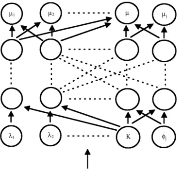
The neural network architecture is varied according to the problem underconsi-deration. Figure 2 shows the general architecture used. The inputs presented to the network at the input layer are the average job interarrival time, the due date tight-ness factor and the queue waiting discipline. The outputs of the network would be the system performance measure of interest. The number of hidden layers and the number of nodes at each layer are varied empirically according to the problem at
hand. Note that too many nodes in hidden layers cause the network to memorize rather than to learn. By the same token, too few nodes result in no learning. Hence, the size of the hidden layer is determined as a result of pilot runs. For example, for estimating the mean job tardiness for a simple deterministic system, three network architectures were tested and the best result was considered. These architectures were 5-6-7-6-3 , 5-8-9-8-3 and 5-55-3 (where the ®rst digit represents the number of nodes in the input layer, the last digit represents the number nodes in the output layer and the digits in between represent the number of nodes per hidden layer). For the complex system con®guration, the network sizes where increased to 8-12-14-12-6 , 8-15-19-15- 6 and 8-45-6.
In the experiments, three network architectures were implemented and the best one was selected for comparison. The back propagation networks operate with a learning coe cient and a momentum term, which are both empirically set. These coe cients remain constant throughout the training session, which has a length of 500 000 input±output combinations (the available data set is presented a multiple number of times). For simplicity, no bias has been introduced to the networks.
An essential aspect of metamodelling is to evaluate the quality of the estimate of the system performance measure (produced by the neural network metamodel) as compared with the true value (produced by the simulation models). For estimating mean machine utilization, two criteria are used: mean absolute deviation (MAD) and percentage error (%error). MAD consists of computing the absolute di erence between each estimate and the true value and these di erences are then averaged across all the output nodes and all the examples in the data set. The percentage error approach is the classic one where the absolute di erence is divided by the true value.
m1 m2 mj l1 l2 K fj m Output Layer Input Layer Hidden Layers Inputs
Figure 2. General neural network architecture.
For estimating mean job tardiness, the classic percentage error approach cannot be used (since tardiness can have a zero value). For this reason, another error assess-ment criterion is employed in the experiassess-ments. We divide the di erence by the ¯ow allowance (as assigned when setting the due dates). This will be denoted as FA. 4. Results of the experiments
4.1. Estimating long-term machine utilization
The ®rst set of experiments is designed to measure metamodel accuracy in esti-mating long-term machine utilization. The results are depicted in ®gures 3±6. Figures 3 and 4 display the errors obtained on the training set for a system with medium demand level. Figures 5 and 6 show the increase in the error levels of the metamodels when the test data sets are used, i.e. graphs plot the error on the test data set minus error on training data set.
In general, the neural network metamodels perform well to estimate mean machine utilization (note that utilization is measure on a scale of 1). It appears
0 . 0 0 0 . 0 1 0 . 0 2 0 . 0 3 N o n e ( d et er m i n i st i c ) I n t er a r r i va l s t i m es o n l y P r o c es s i n g t i m es o n ly B o t h S t o c h a s t i c f a c t o r s S i m p l e S y s t e m C o m p l ex S y s t em
Figure 3. E ect of stochasticity and complexity (training data).
0 % 2 % 4 % N o n e ( d et e r m i n i st i c ) I n t er a r r i va l s t i m es o n l y P r o c es s i n g t i m es o n ly B o t h S t o c h a s t i c f a c t o r s S i m p l e sy s t e m C o m p l e x s y s t e m
Figure 4. E ect of stochasticity and complexity (training data).
that the metamodel accuracy decreases as system complexity increases both on the training and test data sets. It is also noted that the accuracy decreases as a result of adding stochasticity to the system. An interesting result is that the stochastic factors examined in this study yield similar error levels as illustrated by the almost ¯at middle portion in ®gures 3±6. When both variables (interarrival times and processing time) are stochastic, the error increases relative to when only one of them is stoch-astic (®gure 3 and 4). However, the deterioration in metamodel accuracy is almost the same when either one of the variables stochastic (®gures 5 and 6).
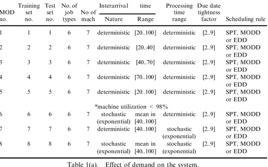
We also examine the e ect of variation in the demand levels on metamodel accuracy. The complex deterministic system is considered with three levels of demand. Tables 1a and b shows the error achieved by the metamodels for both error assessment criteria. It appears that increasing demand levels result in reduced metamodel accuracy both on the training and test data sets. However, this deterio-ration in metamodel accuracy is very small compared with the deteriodeterio-ration due to the added system complexity or stochasticity.
The ability of the metamodel to estimate machine utilization when inputs are outside the range of the training data set is interesting to observe. At this stage, the
0 . 0 0 0 . 0 1 0 . 0 2 0 . 0 3 N o n e ( d et er m i n i st i c ) I n t er a r r i va l s t i m es o n l y P r o c e s si n g t i m e s o n l y B o t h S t o c h a s t i c f a c t o r s S i m p l e S y s t e m C o m p l e x S y st e m
Figure 5. E ect of stochasticity and complexity (error on test data ± error on training data).
0 . 0 % 2 . 0 % 4 . 0 % N o n e ( d e t e r m i n i s t i c ) I n t er a r r i v a l s t i m es o n l y P r o c e s si n g t i m e s o n l y B o t h S t o c h a s t i c f a c t o r s S i m p l e s y st e m C o m p l e x s y s t e m
Figure 6. E ect of stochasticity and complexity (error on test data ± error on training data).
simple deterministic system was considered. Table 2 shows the metamodel accuracy on three test data sets. The ®rst set (®rst row) corresponds to data set with inputs generated from the same range as the training data set (job interarrival times gen-erated from interval [10,85]). The second data set corresponds to input gengen-erated from a range adjacent to the training range (job interarrival times generated from [85,100]). Similarly, the third data set corresponds to inputs generated from a range adjacent to the range of the second data set (job interarrival times are generated from [100,120]. These ranges correspond to testing a neural metamodel built for a system with low demand levels and that is required to extrapolate on higher demand levels. As table 2 shows the metamodel accuracy has a slow degradation outside the train-ing range. This indicates that neural metamodels are robust to changes in operattrain-ing conditions.
Training Test No. of Interarrival time Processing Due date MOD set set job No of time tightness
no. no. no. types mach Nature Range range factor Scheduling rule 1 1 1 6 7 deterministic [20..100] deterministic [2..9] SPT, MODD
or EDD 2 2 2 6 7 deterministic [20..40] deterministic [2..9] SPT, MODD
or EDD 3 3 3 6 7 deterministic [40..70] deterministic [2..9] SPT, MODD
or EDD 4 4 4 6 7 deterministic [70..100] deterministic [2..9] SPT, MODD
or EDD 5 5 5 6 7 deterministic [20..100] deterministic [2..9] SPT, MODD
or EDD *machine utilization < 98%
6 6 6 6 7 stochastic mean in deterministic [2..9] SPT, MODD (exponential) [40..100] or EDD 7 7 7 6 7 deterministic [40..100] stochastic [2..9] SPT, MODD
(exponential) or EDD 8 8 8 6 7 stochastic mean in stochastic [2..9] SPT, MODD
(exponential) [40..100] (exponential) or EDD
Table 1(a). E ect of demand on the system.
Training data Deterioration on test data
Demand level MAD % Error MAD % Error
High 0.0036 0.4 0.0008 0.1
Medium 0.0027 0.4 0.0002 0.0
Low 0.0009 0.5 0.0010 0.0
Table 1(b). E ect of demand on the system.
Set MAD Mean % error
1 0.006 1.4
2 0.04 3.8
3 0.06 5.3
Table 2. Generalization outside the experiment range.
We also observe both error assessment criteria produced consistent results in the experiments. In other words, the di erent models would rank similarly for each criterion. This consistency is a good point as it con®rms the conclusions made so far. In short, the results indicated that neural network metamodels designed to estimate long-term mean machine utilization are quite successful and can handle system stochasticity and complexity.
4.2. Estimating long-term job tardiness
This section examines the capability of neural networks to estimate long-term job tardiness at two levels of system complexity. MAD and FA are used to assess net-work accuracy. Recall that due date related criteria are commonly used in practice to measure the system performances and the mean tardiness is the popular one in the literature.
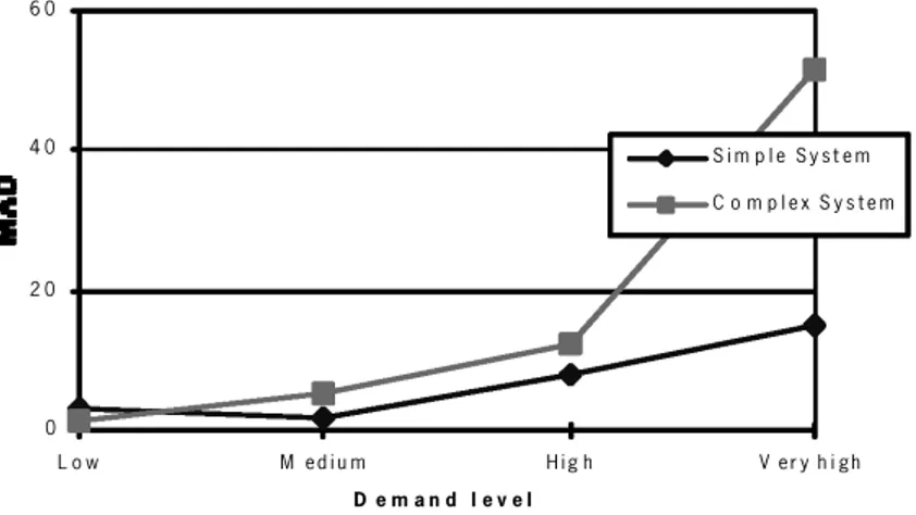
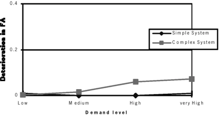
The results are plotted in ®gures 7±14. It appears that neural network metamo-dels are better at estimating long-term machine utilization than estimating long-term
0 2 0 4 0 6 0 L o w M e d i u m H i g h V e r y h i g h D e m a n d l e v e l S i m p l e S y s t e m C o m p l e x S y s t e m
Figure 7. E ect of complexity and demand (training data).
0 0 .2 0 .4 L o w M e d i u m H i g h V e r y h i g h D e m a n d l e v e l S i m p l e S y s t e m C o m p l e x S y s t e m
Figure 8. E ect of complexity and demand (training data).
0 2 0 4 0 6 0 L o w M e d i u m H i g h V e r y h i g h D e m a n d l e v e l S i m p l e S y s t e m C o m p l e x S y s t e m
Figure 9. E ect of complexity and demand (error on test data ± error on training data).
0 0 . 2 0 . 4 L o w M e d i u m H i g h v e r y H i g h D e m a n d l e v e l S i m p l e S y s t e m C o m p l e x S y s t e m
Figure 10. E ect of complexity and demand (error on test data ± error on training data).
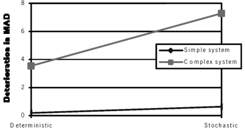
0 2 4 6 8 D et e rm i n i s t i c S t o c h a s t i c S y s t e m t y p e S i m p l e s y s t e m C o m p l e x s y s t e m
Figure 11. E ect of stochasticity and complexity (training data).
0 % 2 % 4 % 6 % D e te r m i n i st i c S t o c h a s t i c Sys t e m t y p e S i m p l e s y s t e m C o m p l e x s y s t e m
Figure 12. E ect of stochasticity and complexity (training data).
0 2 4 6 8 D et e rm i n i s t i c S t o c h a s t i c Sys t e m t y p e S i m p l e s y s t e m C o m p l e x s y s t e m
Figure 13. E ect of stochasticity (error on test data ± error on training data).
0 % 2 % 4 % 6 % D et e rm i n i s t i c S t o c h a s t i c Sys t e m t y p e S i m p l e s y s t e m C o m p l e x s y s t e m
Figure 14. E ect of stochasticity (error on test data ± error on training data).
job tardiness. According to the FA error assessment criteria, the job tardiness is within 10% of ¯ow allowance (for a system in steady-state) . This could be considered as acceptable since there is still room to improve metamodel accuracy through further ®ne-tuning of the metamodel parameters (i.e. by changing network architec-tures and algorithms’ learning and momentum coe cients).
The ®rst point of interest was to examine the e ect of variations in demand levels on metamodel accuracy. Figures 7 and 8 show the error levels achieved by the metamodels for four demand levels on the training data set (based on a deterministic system). Figures 9 and 10 show the degradation in error levels when metamodels are evaluated based on the test data sets. Low demand levels correspond to a data set where the mean of the distribution of the interarrival time is large compared with the case with medium, high or very high demand. Originally, the means of the distribu-tions of the interarrival times were randomly generated from within a large interval. To study the e ect of di erent demand levels, this interval was divided into four non-overlapping subintervals, corresponding to low, medium, high and very high demand levels.
These ®gures illustrate a non-linear deterioration in metamodel accuracy and generalization capability with the most signi®cant deterioration occurring in the very high demand case. The impact of increasing demand levels is most signi®cant for the complex system con®guration. The very high demand case is the case where the training and test sets contain examples for which the system is not in a steady-state. In such a situation, long queues build up and several machines become bottle-necks. As a comparison, in the high demand case, the maximum machine utilization in the examples included in the data sets is 98%. This indicates that metamodels are accurate enough as long as the system is in steady-state . However, as illustrated by ®gures 9 and 10, the increased demand levels do not have such a signi®cant impact on amplifying the error level on the test data sets.
Figures 11 and 12 show the e ect of stochastic interarrival times and processing times on metamodel accuracy, and ®gures 13 and 14 show the e ect of stochasticity on the error deterioration on test sets. We observe that adding stochastic elements to the model reduces metamodel accuracy and ampli®es error deterioration. This impact is further ampli®ed by having more complex system con®guration.
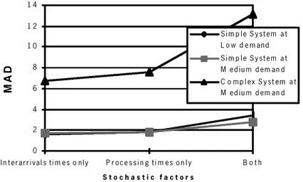
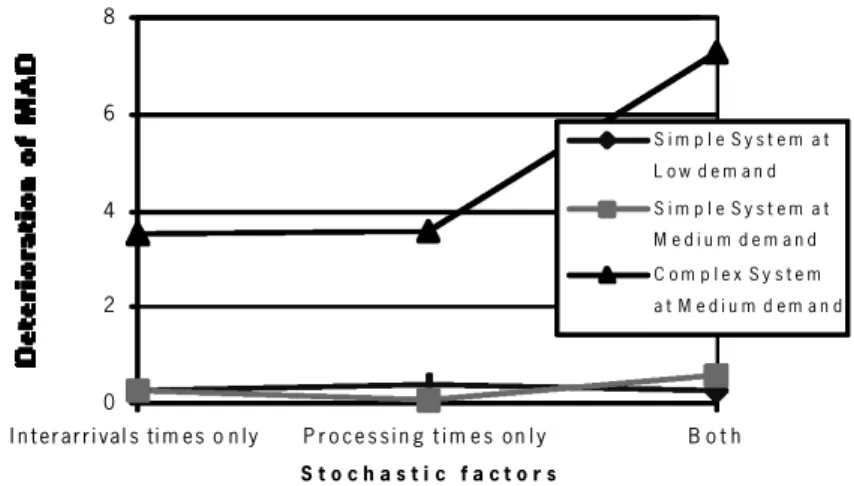
Figures 15 and 16 depict the impact of stochasticity on metamodel accuracy in more detail. Figures 17 and 18 show the e ect of di erent stochastic variables on degradation in a metamodel error on the test data set. When processing times are stochastic, the metamodels have achieved slightly higher error levels than when interarrival times are stochastic. When both variables are stochastic, metamodel accuracy decreases sharply. Once again, system complexity ampli®es error levels signi®cantly.
4.2.1. Machine breakdowns
The systems modelled so far are not subject to machine breakdowns. Hence, one may question the robustness of the metamodels with respect to random breakdown interruptions (i.e. can a metamodel trained on a system with a 100% e ciency, generalize to examples from the same system but subject to machine breakdowns?). To perform this test, we reduce the machine e ciency to 92%. Tables 3 and 4 display the results in terms of the level of error achieved by the metamodels on the test data set both simple and complex systems and for the two error assessment criteria.
It appears that the robustness of the metamodels to machine breakdown is highly dependent on system complexity and the demand on the system and to a lesser extent on stochasticity. The most signi®cant deterioration is observed at the highest demand and at the complex system. Analysing the data for this situation indicates that machine breakdowns cause large queues to form, which in turn does not allow the system to reach its steady-state equilibrium.
4.3. Estimating short-term job tardiness
This section investigates the potential use of neural network to estimate short-term performance of the system. In this type of situation, the analyst wants to estimate the system performance for a certain period given well-de®ned initial con-ditions, e.g. given the number of jobs and machines with current load, to estimate job
0 2 4 6 8 1 0 1 2 1 4 I n t er ar r i val s t i m es o n l y P r o ce s s i n g t i m es o n l y B o t h S t o c h a s t i c f a c t o r s M A D S i m p l e S y st em a t L o w d e m an d S i m p l e S y st em a t M ed i u m d em an d C o m p l ex S y st em a t M ed i u m d em an d
Figure 15. E ect of stochasticity, demand and complexity (training data).
0 % 2 % 4 % 6 % 8 % 1 0 % I n t er a r r i va l s t i m es o n ly P r o ces s i n g t i m es n o n l y B o t h S t o c h a s t i c f a c t o r s S i m p l e S y st em a t L o w d e m an d S i m p l e S y st em a t M ed i u m d em an d C o m p l e x S y s t e m a t M ed i u m d em an d
Figure 16. E ect of stochasticity, demand and complexity (training data).
0 2 4 6 8 I n t er ar r i val s ti m es o n l y P r o ce s s i n g t i m e s o n l y B o t h S t o c h a s t i c f a c t o r s S i m p l e S y s t e m a t L o w d e m a n d S i m p l e S y s t e m a t M e d i u m d e m a n d C o m p l e x S y s t e m a t M e d i u m d e m a n d
Figure 17. E ect of stochasticity, demand and complexity (error on test data ± error on training data). 0 % 2 % 4 % I n t er a r r i va l s t i m es o n ly P r o ce s s i n g t i m es o n l y B o t h S t o c h a s t i c f a c t o r s S i m p l e S y s t e m a t L o w d e m a n d S i m p l e S y s t e m a t M e d i u m d e m a n d C o m p l e x S y s t e m a t M e d i u m d e m a n d
Figure 18. E ect of stochasticity, demand and complexity (error on test data ± error on training data).
Deterministic system Stochastic system
Low Medium High Low Medium
demand demand demand demand demand
MAD approach with breakdowns 3.3 0.8 104.8 6.1 7.3
without breakdowns 3.0 1.6 15.0 3.6 3.1
FA approach with breakdowns (%) 5.7 0.4 45.7 9.2 3.5 without breakdowns (%) 4.0 2.1 2.7 2.7 2.9 Table 3. Simple system: robustness to machine breakdowns.
completions or job tardiness. Since the initial system status is now a relevant factor in the system, new nodes are added to the input layer of the neural networks. The information about initial system status is incorporated into the model in terms of the work in progress inventory of each job type waiting before each machine in the system.
The results of experiments are presented in ®gures 19±22. The curve titled `gen-eralization’ in these ®gures represents the di erences between metamodel errors on test and training sets. As expected, stochasticity and system complexity act nega-tively on the metamodel performance and its generalization capability. The results for the complex stochastic system con®guration are not shown because the errors are very high. It appears that system complexity has a more negative e ect on the system performance than stochasticity. This signi®cant increase in error level in stochastic systems indicated that neural networks might not be suitable for estimating short-term performance of the systems when the level of variation and stochastic elements are high.
The e ect of demand on system performance is displayed ®gures 21 and 22. It appears that the higher the demand, the better is the metamodel accuracy and gen-eralization capability. This result was unexpected since for estimating long-term job-tardiness, we found that increasing demand (or load on the system) resulted in a decreased accuracy of the metamodels. In this set of experiments, increasing the Deterministic system Stochastic system
Low Medium High Low Medium
demand demand demand demand demand MAD approach with breakdowns 3.3 36.3 277.0 9.0 55.6
without breakdowns 1.3 5.4 51.8 13.2 13.2 FA approach with breakdowns (%) 2.9 21.2 178.8 7.0 27.5
without breakdowns 1.2 3.7 46.1 8.0 8.0
Table 4. Complex system: robustness to machine breakdowns.
0 5 0 1 0 0 1 5 0 2 0 0 si m p l e d et er m i n i st i c s y s t em s i m p l e st o c h a s t i c sy s t e m c o m p l ex d et e r m i n i s t i c s y s t e m Sys t e m ty p e M A D T r a i n i n g s et T e s t s e t G en er a li z a t i o n
Figure 19. E ect of stochasticity and complexity.
0 % 5 0 % 1 0 0 % 1 5 0 % 2 0 0 % si m p l e d et erm i n ist i c s y st em si m p l e st o c h a st i c s y s t em c o m p l ex d et er m i n i st i c s y s t e m Sys t e m t y p e F A T r a i n i n g s et T es t s et G en era l i za t i o n
Figure 20. E ect of stochasticity and complexity.
0 2 0 4 0 6 0 8 0 1 0 0 h ig h m ed iu m De m a n d M A D T e s t s et E r r o r d e t er i o r a t i o n
Figure 21. E ect of demand level.
0 % 1 0 % 2 0 % 3 0 % h i g h l o w De m a n d F A T e s t s e t E r r o r d e t e r i o r a t i o n
Figure 22. E ect of demand level.
demand resulted in a higher accuracy level. The interpretation made sense at the time. In estimating short-term job tardiness, the system is not in steady-state , but there is a degree of how far it is from its steady-state . The interpretation of these results is that at high demand, the system is nearer to its steady-state than with lower demand. The idea is that because of the stability of the system, steady-state perform-ance is easier to predict. We saw in the previous experiments (long-term) that the more the system is overloaded, the worst the accuracy. Similarly, in this case (short-term), the more the system is under-loaded, the worse its accuracy. We can view demand as on a line: in the middle, we have the range of the demand where the system is in steady-state . In this interval, the metamodel accuracy is good. The more we move the right or to the left of this interval, the worst is the metamodel accuracy. The previous experiments showed that the quicker the system can tend towards its steady-state equilibrium, the better is the metamodel accuracy. However, these experiments assumed that all machine queues are empty initially.
Next, we investigated the e ect of the initial system status for variable demand on system, by ®xing the number of jobs (from each job type) in each queue. The results are displayed for the cases where demand level is high, medium or both combined (referred to as general). As seen in ®gures 23 and 24, increasing the initial number of jobs in the queues results in improving the results until some point then no improvement is observed. The points at which the error levels level o correspond approximately to the average number of jobs in the queue when the system is at state . Even if this initial number exceeds the average queue size at steady-state, metamodel performance does not change. The same e ect of the initial system status exists when we split the range of the interarrival times to low demand and to high demand.
The e ect of initial system status on metamodel generalization capability is shown in ®gures 25 and 26. As can be seen, the deterioration in error levels does not have a speci®c pattern.
The purpose of using neural metamodels to estimate short-term tardiness was to investigate their possible use in a real-time decision. One situation frequently encountered in the real-life scheduling practices is to select the best scheduling rule
0 10 20 30 40 50 60 70 10 15 20 25 Initial # of job s p e r ma ch in e M A D M edium demand Hi g h deman d G en eral
Figure 23. E ect of initial system status (trainind data).
0% 4% 8% 12% 16% 10 15 20 25 Initial # of job s p e r m a ch in e F A M ediu m deman d Hi g h deman d G eneral
Figure 24. E ect of initial system status (trainind data).
0 1 2 3 4 10 15 20 25
Initial # of job s p e r m ac h ine
M A D M ediu m deman d Hi g h deman d G en eral
Figure 25. E ect of initial system status (error on test data ± error on training data).
0% 1% 2% 3%
10 15 20 25
In itial # of job s p e r ma c hin e
F
A
M ediu m demand Hi g h deman d G en eral
Figure 26. E ect of initial system status (error on test data ± error on training data).
or dispatching policy based on the information about the current state of system and objectives. For that reason, we conducted another sets of experiments to see if one can make good decisions via neural networks. In other words, we wanted to know if, based on the metamodel, we would select the same dispatching rule, as we would do if we base the decision on the simulation model. This test is applied on three general models, corresponding to deterministic simple system stochastic simple system, and deterministic complex system. In selecting the dispatching rule (based on the simula-tion models or on the neural metamodel), several alternatives are available. If the job types have di erent weights, then we may select the dispatching rule that minimizes the tardiness of the job type with highest weight. This may be the case when one job type is very pro®table or very strategic to the business. Another alternative would be to select the rule that produces the minimum overall average tardiness (across all the job types).
Table 5 shows the results of these experiments. Entries represent the percentage of the example in the test data set for which the correct decision was made by the metamodel. The columns correspond to di erent decision criteria. For example, the ®rst column corresponds to the case where the objective is to select the dispatching rule that best minimizes tardiness for job type 1 (and similarly for columns 2±6). The last column corresponds to the case where the objective is to select the dispatching rule that best minimized the overall tardiness.
In the previous experiments, we observed that stochasticity and system complex-ity have negative e ects on the accuracy of the metamodel. However, the results in this section give the opposite indications. The di erence lies on the how the meta-model is evaluated. While in the previous experiments, the metameta-models were eval-uated on their capacity to forecast the performance measures of the manufacturing system, in this section the metamodels were evaluated on their capacity to rank the performance of di erent queuing rules, which would allow us to select the best queuing rule.
If the selection of the queuing rule is based on the overall average tardiness, the metamodel success rate on the complex deterministic system ranks better than on the simple stochastic system, which in turn ranks better than on the simple deterministic system. The reason for this contradiction may be that complexity (whether due to stochasticity or to system con®guration) acts as to increase the di erence between the performances of the di erent dispatching rules. In other words, the added complex-ity makes it more di cult to forecast the value of the performance measures. However, under these same conditions of added complexity, it is easier to di erenti-ate between the performances of the di erent queuing rules. Thus, it may be easier
Job type
System 1 2 3 4 5 6 Average
Simple, stochastic 96 84 49 n.a. n.a. n.a. 91
Simple, deterministic 81 100 79 n.a. n.a. n.a. 79
Complex, deterministic 100 100 71 97 98 100 100
Data are percentages. n.a., not applicable.
Table 5. Testing capability to select operational policies.
for the metamodel to compare di erent queuing rules rather than provide precise measures of the performance of each rule. This implies that using neural metamodel is likely to produce good decisions as the system gets more complex. In addition, the test results show that making the decisions based on di erent job types leads to di erent metamodel performances. It appears that the metamodel performance is related to the job type characteristics. The results also indicated that di erent criteria lead to opposite interpretations or di erent decisions. Hence, the choice of the criteria should depend on the objective of the study.
5. Concluding remarks and future research directions
In this paper, we have conducted an initial investigation of the potential use of neural networks as simulation metamodels for estimating manufacturing system per-formances. The experiments indicated that application to real-life problems is not straightforward. We also observed that performance measures, the study horizon, the system load, the initial system status, stochasticity, complexity and error assess-ment methods can a ect metamodel accuracy in di erent ways. For example, experiments indicated that metamodel accuracy can decrease rapidly when estimating short-term job tardiness for terminating type systems in the context of stochastic or complex systems. However, the metamodels were successful in discriminating between dispatching policies in this same contexts. Therefore, the success of metamodelling with neural networks depends on the combination of the system characteristics and the error assessment criteria, as well as the purpose of simulation applications.
In conclusion, we believe that metamodelling with neural networks is a promising tool and can be of value for manufacturing systems’ management. To investigate further the potential of this tool, one can examine the e ect of system con®guration (¯ow shop to job shop), system disturbances such as machine break down, applying di erent distributions in studying stochasticity, the size of data sets, or estimating other measures such as the standard deviation of the performance measures.
References
Aussem, A. and Hill, D., 2000, Neural-network metamodeling for the prediction of Caulerpa taxifolia development in the Mediterranean sea. Neurocomputing, 30, 71±78. Badiru, A. B. and Sieger, D. B., 1998, Neural network as a simulation metamodel in
economic analysis of risky projects. European Journal of Operational Research, 105, 130±142.
Barton, R. R., 1992, Metamodeling for simulation input-output relations. Proceedings of the
1992 Winter Simulation Conference.
Blanning, R. W., 1975, The construction and implementation of metamodeling. Simulation, 24, 177±184.
Burke, L. I. and Ignizio, J. P., 1992, Neural networks and operation research: an overview.
Computer Operations Research, 19, 179±189.
Chryssolouris, G., Lee, M. and Domroese, M., 1991, The use of neural networks in deter-mining operational policies for manufacturing systems. Journal of Manufacturing
Systems, 100, 166±175.
Chryssolouris, G., Lee, M., Pierce, J. and Domroese, M., 1990, Use of neural networks for the design of manufacturing systems. Manufacturing Review, 3, 187±194.
Dayhoff, J. E., 1990, Neural Network Architectures: an Introduction (New York: Van Nostrand Reinhold).
Fishwick, P. A., 1989, Neural network models in simulation: a comparison with traditional modeling approaches. Proceedings of the 1989 Winter Simulation Conference, pp. 702± 710.
Freidman, L. W. and Pressman, I., 1988, The metamodeling in simulation analysis: can it be trusted? Journal of the Operational Research Society, 39, 939±948.
Harmonosky, C. M. and Robohn, S. F., 1995, Investigating the application potential of simulation for real time control decisions. International Journal of Computer
Integrated Manufacturing, 8, 126±132.
Huang, C. L., Huang, Y. H., Chang, T. Y., Chang, S. H., Chung, C. H., Huang, D. T. and Li, R. K., 1999, The construction of production performance prediction system for semiconductor manufacturing with arti®cial neural networks. International Journal
of Production Research, 37.
Hurrion, R. D., 1992, Using a neural network to enhance the decision making quality of a visual interactive simulation model. Journal of Operational Research Society, 43, 333± 341.
Hurrion, R. D., 1997, An example of simulation optimization using a neural network meta-model: ®nding the optimum number Kanbans in a manufacturing system. Journal of the
Operational Research Society, 48, 1105±1112.
Hurrion, R. D., 1998, Visual interactive meta-simualtion using neural networks.
International Transactions Operational Research, 5, 261±271.
Hurrion, R. D. and Birgil, S., 1999, Comparison of factorial and random experimental design methods for the development of regression and neural network simulation meta-models. Journal of the Operational Research Society, 50, 1018±1033.
Kilmer, R. A., Smith, A. E. and Shuman, L. J., 1999, Computing con®dence intervals for stochastic simulation using neural network neural network. Computers and Industrial
Engineering, 36, 391±407.
Kleijnen, J. P. C. and Sargent, R. G., 2000, A methodology for ®tting and validating metamodels in simulation. European Journal of Operational Research, 120, 14±29. Madey, G. R., Weinrth, J. and Shah, V., 1992, Integration of neurocomputing and system
simulation for modeling continuous improvement systems in manufacturing. Journal of
Intelligent Manufacturing, 3, 193±204.
McHaney, R. W. and Douglas, D. E., 1997, Multivariate regression metamodel: a DSS application in industry. Decision Support Systems, 19, 43±52.
Mollaghasemi, M., LeCroy, K. and Georgiopoulos, M., 1998, Application of neural networks and simulation modeling in manufacturing system design. Interfaces, 28, 100±114.
Philipoom, P. R., Rees, L. P. and Wiegmann, L., 1994, Using neural networks to determine internally set due date assignments for shop scheduling. Decision Sciences, 25, 825±851. Pierreval, H., 1992, Rule based simulation metamodels. European Journal of the Operational
Research Society, 61, 6±17.
Pierreval, H., 1993, Neural network to select dynamic scheduling heuristics. Revue des
SysteÁmes de DeÂcision, 2, 173±190.
Pierreval, H., 1996, A metamodeling approach based on neural networks. International
Journal of Computer Simulation, 6, 365±378.
Raaymakers, M. H. M. and Weijters, A. J. M. M., 2000, Using regression models and neural network models for makespan estimation in batch processing. In van der Bosch and H. Weigand (Eds., Proceedings of the Twelfth Belgium±Netherlands Conference on AI, pp. 141±148.
Sabuncuoglu, I., 1998, Scheduling with neural networksÐa review of the literature and new research directions. Production and Inventory Control, 9, 2±12.
Sabuncuoglu, I. and Hommertzheim, D., 1995, Experimental investigation of an FMS due-date scheduling problem: an evaluation of due-due-date assignment rules. International
Journal of Computer Integrated Manufacturing, 8, 133±144.
Watson, E. F., Chawda, P. P., McCarthy, B., Drevna, M. J. and Sadowski, R. P., 1998, A simulation metamodel for response-time planning. Decision Sciences, 29, 217±241. Yu, B. and Poplewell, K., 1994, Metamodeling in manufacturing: a review. International
Journal of Production Research, 32, 787±796.
Zhang, H. C. and Huang, S. H., 1995, Applications of neural networks in manufacturing: a state of the art survey. International Journal of Production Research, 33, 705±728.