Model based methods for the control and planning of running robots

MODEL BASED METHODS FOR THE CONTROL

AND PLANNING OF RUNNING ROBOTS

a thesis

submitted to the department of electrical and

electronics engineering

and the institute of engineering and sciences

of bilkent university

in partial fulfillment of the requirements

for the degree of

master of science

By

¨

Om¨ur Arslan

July 2009

I certify that I have read this thesis and that in my opinion it is fully adequate, in scope and in quality, as a thesis for the degree of Master of Science.

Prof. Dr. ¨Omer Morg¨ul(Supervisor)

I certify that I have read this thesis and that in my opinion it is fully adequate, in scope and in quality, as a thesis for the degree of Master of Science.

Assist. Prof. Dr. Uluc. Saranlı(Co-supervisor)

I certify that I have read this thesis and that in my opinion it is fully adequate, in scope and in quality, as a thesis for the degree of Master of Science.

Prof. Dr. Hitay ¨Ozbay

I certify that I have read this thesis and that in my opinion it is fully adequate, in scope and in quality, as a thesis for the degree of Master of Science.

Assist. Prof. Dr. Afs.ar Saranlı

Approved for the Institute of Engineering and Sciences:

Prof. Dr. Mehmet Baray

ABSTRACT

MODEL BASED METHODS FOR THE CONTROL

AND PLANNING OF RUNNING ROBOTS

¨

Om¨ur Arslan

M.S. in Electrical and Electronics Engineering

Supervisor: Prof. Dr. ¨

Omer Morg¨ul

July 2009

The Spring-Loaded Inverted Pendulum (SLIP) model has long been established as an effective and accurate descriptive model for running animals of widely differing sizes and morphologies. Not surprisingly, the ability of such a simple spring-mass model to capture the essence of running motivated several hopping robot designs as well as the use of the SLIP model as a control target for more complex legged robot morphologies. Further research on the SLIP model led to the discovery of several analytic approximations to its normally nonintegrable dynamics. However, these approximations mostly focus on steady-state running with symmetric trajectories due to their linearization of gravitational effects, an assumption that is quickly violated for locomotion on more complex terrain wherein transient, non-symmetric trajectories dominate. In the first part of the thesis , we introduce a novel gravity correction scheme that extends on one of the more recent analytic approximations to the SLIP dynamics and achieves good accuracy even for highly non-symmetric trajectories. Our approach is based on incorporating the total effect of gravity on the angular momentum throughout a single stance phase and allows us to preserve the analytic simplicity of the approximation to support research on reactive footstep planning for dynamic

legged locomotion. We compare the performance of our method with two other existing analytic approximations by simulation and show that it outperforms them for most physically realistic non-symmetric SLIP trajectories while main-taining the same accuracy for symmetric trajectories. Additionally, this part of the thesis continues with analytical approximations for tunable stiffness control of the SLIP model and their motion prediction performance analysis. Similarly, we show performance improvement for the variable stiffness approximation with gravity correction method. Besides this, we illustrate a possible usage of approx-imate stance maps for the controlling of the SLIP model.

Furthermore, the main driving force behind research on legged robots has always been their potential for high performance locomotion on rough terrain and the outdoors. Nevertheless, most existing control algorithms for such robots either make rigid assumptions about their environments (e.g flat ground), or rely on kinematic planning with very low speeds. Moreover, the traditional separation of planning from control often has negative impact on the robustness of the system against model uncertainty and environment noise. In the second part of the thesis, we introduce a new method for dynamic, fully reactive footstep planning for a simplified planar spring-mass hopper, a frequently used dynamic model for running behaviors. Our approach is based on a careful characterization of the model dynamics and an associated deadbeat controller, used within a sequential composition framework. This yields a purely reactive controller with a very large, nearly global domain of attraction that requires no explicit replanning during execution. Finally, we use a simplified hopper in simulation to illustrate the performance of the planner under different rough terrain scenarios and show that it is robust to both model uncertainty and measurement noise.

Keywords: Footstep Planning, Legged Locomotion, Hybrid System, Reactive

Control, Approximate Stance Map, Spring-Mass Hopper, Rough Terrain, Non-symmetric Steps

¨

OZET

KOS¸AN ROBOTLARIN KONTROL VE PLANLAMASI ˙IC

¸ ˙IN

MODEL TABANLI Y ¨

ONTEMLER

¨

Om¨ur Arslan

Elektrik ve Elektronik M¨uhendisli¯gi B¨ol¨um¨u Y¨uksek Lisans

Tez Y¨oneticisi: Prof. Dr. ¨

Omer Morg¨ul

Temmuz 2009

Y¨ukl¨u Yay Ters Sarka¸c (YYTS) modeli ¸cok de˘gi¸sik boyut ve morfolo-jideki ko¸san hayvanların etkili ve g¨uvenilir tanımlayıcı modellenmesinde uzun s¨uredir kullanıldı˘gı gibi de˘gi¸sik zıplayan robotların tasarımı i¸cin de bir ta-ban olu¸sturmaktadır. Bu model ¨uzerindeki ilerleyen ara¸stırmalar integrali alınamayan dinami˘gi i¸cin de˘gi¸sik analitik yakla¸sıklamalar ile sonu¸clanmı¸stır. Yer¸cekimi etkisinin do˘grusalla¸stırılmasından dolayı bu yakla¸sıklamalar ¸co˘gunlukla kararlı durumdaki simetrik ko¸smalara yo˘gunla¸smı¸stır, ancak bu varsayım ge¸cici rejim ve simetrik olmayan gezingelerin sıklıkla kullanıldı˘gı karma¸sık y¨uzeylerde bozulmaktadır. Bu tezin ilk kısmında, yeni bir yer¸cekimi etkisini d¨uzeltme y¨ontemi tanıtılmı¸s ve varolan analitik YYTS dinami˘gi yakla¸sıklamasının g¨uvenilirli˘gi olduk¸ca fazla simetrik olmayan gezingeler i¸cin arttırılmı¸stır. Yakla¸sımımız bir adım sırasında yer¸cekiminin a¸cısal moment ¨uzerine olan toplam etkisinin yakla¸sıklamaya dahil edilmesine dayanıyor ve b¨oylelikle de bu kolay analitik yakla¸sıklama reaktif adım planlanmasında da kullanılabilir. Y¨ontemimizin performansı litarat¨urde varolan iki analitik yakla¸sıklama ile kar¸sıla¸stırılmı¸s, ¸cok sık kullanılan simetrik olmayan gezingeler i¸cin di˘gerlerinden daha iyi oldu˘gu ve simetrik gezingelerde ise aynı performansa

sahip oldu˘gu g¨ozlenmi¸stir. Buna ek olarak, ayarlanabilir b¨uk¨ulmezlik i¸cin itik yakla¸sıklamalar ve bu yakla¸sıklamaların hareket kestirme performansı anal-izi incelenmi¸stir. Benzer bir ¸sekilde, de˘gi¸sken b¨uk¨ulmezlik yakla¸sıklamasının yer¸cekimi etkisini d¨uzeltme y¨ontemi ile birlikte kullanıldı˘gında belirgin bir per-formans geli¸simi g¨ozlenmi¸stir. Bunun yanısıra, YYTS modelinin kontroll¨unde bu yakla¸smaların olası kullanımını g¨osterdik.

Bacaklı robotlardaki ara¸stırmaların arkasındaki asıl itici g¨u¸c bu robotların karma¸sık y¨uzeylerde ve dı¸s ortamlarda y¨uksek devinim potensiyellerinin ol-masıdır. Buna ra˘gmen, bu robotlar i¸cin varolan kontrol algoritmalarının ¸co˘gu ya ortam ile ilgili katı varsayımlara (d¨uz zemin gibi) yada ¸cok d¨u¸s¨uk hızlarda kinematik planlamaya dayanmaktadır. Planlamanın geleneksel olarak kon-troldan ayrılması genellikle model belirsizli˘gine ve ortam g¨ur¨ult¨us¨une kar¸sı sis-temin dayanıklılı˘gının azalmasına neden olmaktadır. Bu tezin ikinci kısmında, ko¸sma davranı¸sları i¸cin sıklıkla kullanılan dinamik bir model olan basitle¸stirilmi¸s d¨uzlemsel yay-k¨utle sı¸crayanı i¸cin dinamik ve tamamen reaktif adım planlaması i¸cin yeni bir method ¨onerilmektedir. Yakla¸sımımız model dinami˘ginin dikkatli bir ¸sekilde karakterize edilmesine ve sıralı ardı¸sık bile¸sim tasla˘gı i¸cerisinde kul-lanılacak ilgili deadbeat kontrol¨une dayanmaktadır. B¨oylelikle ¸cok geni¸s, hemen hemen evrensel ¸cekim y¨oresi olan ve uygulama sırasında tekrar planlama ihtiyacı duymayan tamamen reaktif denetleyici sa˘glanmı¸s olmaktadır. Son olarak, planlayıcının performansı sim¨ulasyon ortamında ba¸sitle¸stirilmi¸s bir sı¸crayıcının ¨uzerinde de˘gi¸sik y¨uzey ko¸sullarında g¨osterilmi¸s ve y¨ontemin model belirsizlikler-ine ve ¨ol¸cme g¨ur¨ult¨ulerbelirsizlikler-ine kar¸sı dayanıklı oldu˘gunu g¨ozlemlenmi¸stir.

Anahtar Kelimeler: Adım Planlaması, Bacaklı Lokomosyon, Karma Sistem,

Reaktif Kontrol,Y¨ukl¨u Yay Ters Sarka¸c (YYTS), Analitik YYTS Dinami˘gi Yakla¸sıklaması, Karma¸sık Arazi, Simetrik Olmayan Adımlar

ACKNOWLEDGMENTS

First, I would like to thank my supervisors, ¨Omer Morg¨ul and Ulu¸c Saranlı, for their guidance and support throughout my study. This work is an achievement of their invaluable advice. They were always there to listen and to give advice. I am very grateful to my advisor for their patience during our everlasting exciting research meetings and stimulating discussions. Also, I really appreciate all the help they’ve given me to control my interest and deeply study a problem.

I took my initial steps into the area of dynamical legged locomotion with our brilliant and helpful discussions during SensoRhex Project. I am thankful to all the members of SensoRhex Project. This is a great opportunity to express my respect to Af¸sar Saranlı, Ulu¸c Saranlı, Yi˘git Yazıcıo˘glu and Kemal Leblebici o˘glu . Especially, I would like to thank Ulu¸c Saranlı for inspiring me to legged robotics with his endless energy and enthusiasm for legged systems.

Additionally, there are a number of people from my research group, Bilkent Dexterous Robotics and Locomotion (BDRL), who help me along the way. I am very thankful to Akın Avcı (patron - my boss), Tu˘gba Yıldız, Sıtar Kortik and Cihan ¨Ozt¨urk for our wonderful late night studies and discussions. Further thanks should also go to the member of Robotics Laboratory (RoLab) at Middle East Technical University (METU), Mustafa Mert Ankaralı (my great colleague), Emre Ege and G¨okhan G¨ultekin.

I also extend my thanks to my friends from my department, Onur Tan, Vahdettin Ta¸s, Ahmet Sezgin and Fazlı Kaybal, for their invaluable discussions on science, technology, politics and sports.

I am also appreciative of the financial support from Bilkent University, De-partment of Electrical and Electronics Engineering and T ¨UB˙ITAK, the Scientific and Technical Research Council of Turkey.

Finally, but forever I would like to thank my parents, Ali and Arife Arslan, my brother, Onur Arslan, and my little sister, Arzu Arslan, for their love, support and encouragement.

Contents

1 INTRODUCTION 1

1.1 Components of a Robotic System . . . 1

1.2 Legged or Wheeled Systems . . . 2

1.3 Motivation and Existing Work . . . 4

1.4 Methodology . . . 8

1.5 Organization of Thesis . . . 9

2 BACKGROUND: THE SPRING-MASS HOPPER 11 2.1 The SLIP Model . . . 11

2.1.1 The SLIP Template . . . 12

2.1.2 SLIP Dynamics . . . 16

2.1.3 Possible Modes of Control . . . 20

2.2 Approximate Stance Maps . . . 22

2.2.1 Simple Approximate Stance Map by Geyer et al. . . 23

3 MODELLING AND CONTROL OF NONSYMMETRIC SLIP

STEPS 32

3.1 Nonsymmetric Steps During Legged Locomotion . . . 32

3.2 An Approximate Stance Map with Gravity Correction . . . 33

3.2.1 Analytical Approximation Model . . . 33

3.2.2 Performance Analysis . . . 36

3.2.3 Discussion . . . 41

3.3 An Approximate Stance Map for Two-Phase Stiffness Control . . 43

3.3.1 Simple Approximate Stance Map For Two-Phase Variable Stiffness . . . 45

3.3.2 Iterative Approximate Stance Map For Two-Phase Vari-able Stiffness . . . 50

3.3.3 Performances of Proposed Approximations . . . 53

3.3.4 Discussion . . . 61

4 BACKGROUND: CONTROL AND PLANNING OF LEGGED LOCOMOTION OVER ROUGH TERRAIN 64 4.1 Planning and Control of Static and Quasistatic Legged Locomo-tion . . . 65

4.2 Planning and Control of Dynamic Legged Locomotion . . . 66

4.3 Simultaneous Planning and Control via Sequential Composition . 68

5.1 General Form of Deadbeat Controllers . . . 71

5.2 Implementation of Deadbeat Controllers . . . 75

5.3 Applications . . . 79

5.4 Discussion . . . 83

6 REACTIVE FOOTSTEP PLANNING 90 6.1 Planning Framework . . . 91

6.1.1 A Generic Hopper Model . . . 91

6.1.2 Reactive Footstep Planning . . . 94

6.2 Reactive Foorstep Planning of a Simplified Hopper: Ball Hopper . 97 6.2.1 Simplified Hopper Model . . . 98

6.2.2 Simulation Results . . . 104

6.2.3 Discussion . . . 108

List of Figures

1.1 Three main components of a robotic platform: Sensors, Controller, Actuators. . . 1

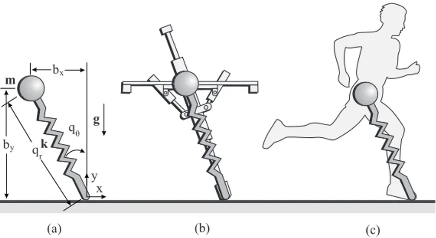
1.2 (a) The SLIP model, (b) Raibert’s hopper, (c) A human runner. 5

1.3 The total gravity effect on the angular momentum at the end of the stance phase compared to touchdown instant: (a) decreasing effect on magnitude, (b) the angular momentum is the same since it is a symmetric gait, (c) increasing effect on magnitude. . . 6

1.4 An illustrative figure of the spring mass hopper locomotion over an uneven terrain (inspired from [1]). . . 7

1.5 A spring-mass hopper running over rough terrain. . . 9

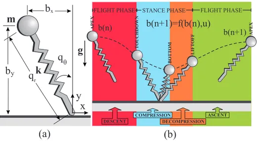
2.1 The SLIP Model. (a) Coordinates and model parameters. (b) Lo-comotion phases (shaded regions) and transition events (bound-aries). . . 12

2.2 The Apex Return Map . . . 16

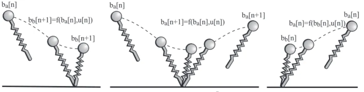
2.3 Left: Apex to Bottom Map. Middle: Apex Return Map. Right: Bottom to Apex Map. . . 23

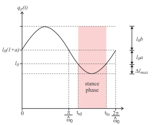
2.4 General solution for the leg length, qr(t), during stance. The si-nusoidal solution has amplitude l0b and frequency ˆω0 with offset l0(1 + a). Since the solution is only suitable for the stance phase,

only the portion where qr ≤ l0 is significant. The parameter a can

also be negative, in which case l0 will be above l0(1 + a). ∆lmax represents the maximum leg compression. (reproduced from [2]) . 25

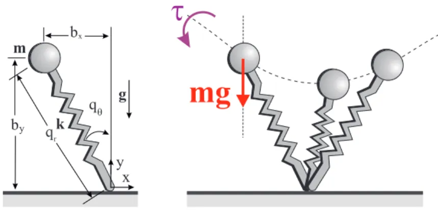
3.1 The total gravity effect on the angular momentum at the end of the stance phase compared to the touchdown instant (blue and red regions represent decreasing and increasing effects of gravity, respectively). (a) decreasing effect on magnitude, (b) angular mo-mentum stays the same due to the symmetric step, (c) increasing effect on magnitude. . . 33

3.2 The effect of gravity on the angular momentum: τ , gravitational torque on the spring-mass hopper . . . 34

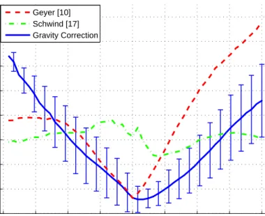
3.3 Approximation performances for the stance maps of Geyer [2],

Schwind [3] and our proposed Gravity Correction method. P Eap

(left) and P Elov (right) are apex position and liftoff velocity per-centage errors. Empty markers, filled markers and colored vertical bars represent mean, maximum and standard deviations of asso-ciated approximations. . . 38

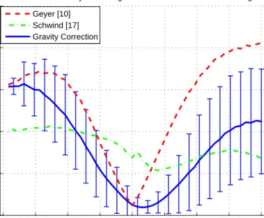
3.4 Mean Apex Position Percentage Error (P Eap) versus Relative Touchdown Angle (qθtd− qθtdn). The vertical bars represent

stan-dard deviations for the approximate stance map with gravity cor-rection. . . 39

3.5 Mean Liftoff Velocity Percentage Error (P Elov) versus Relative Touchdown Angle (qθtd − qθtdn). The vertical bars represent the

standard deviations for the approximate stance map with gravity correction. . . 40

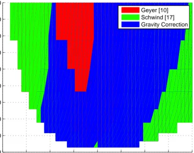
3.6 Comparison of the mean Apex Position Percentage Errors. Col-ored regions show where the associated approximation performs better. . . 41

3.7 Comparison of the mean Liftoff Velocity Percentage Errors. Col-ored regions show where the associated approximation performs better. . . 42

3.8 SLIP apex return map for two-phase variable stiffness case. The two-phase variable stiffness apex return map is composed of the apex to bottom map with compression phase leg stiffness, kc, and the bottom to apex map with decompression phase stiffness, kd. . 44

3.9 Left: Separate Approximate Stance Map for not variable com-pliance with spring constants kc and kd. Middle: Approximate Stance Map for Variable Stiffness with only parameter updates. A discontinuity is observed on stance map at bottom instance. Right: Approximate Stance Map for variable stiffness with param-eter updates and velocity and position state continuity constraints 48

3.10 Estimation performances for the stance maps of Simple, Iterative and Simple Gravity Corrected Variable Stiffness (VS) Approxi-mations. P Eap (left) and P Elov (right) are apex position and liftoff velocity percentage errors. Empty markers, filled markers and colored vertical bars represent mean, maximum and standard deviations of associated approximations. . . 56

3.11 Upper:Mean Apex Position Percentage Error (P Eap) versus Rel-ative Touchdown Angle (qθtd − qθtdn). Lower: Mean Liftoff

Ve-locity Percentage Error (P Elov) versus Relative Touchdown Angle (qθtd − qθtdn). The vertical bars represent standard deviations for

the approximate stance map with gravity correction. . . 57

3.12 Upper:Mean Apex Position Percentage Error (P Eap) versus Stiff-ness Ratio (kd/kc). Lower: Mean Liftoff Velocity Percentage Error (P Elov) versus Stiffness Ratio (kd/kc). The vertical bars represent standard deviations for the approximate stance map with gravity correction. . . 58

3.13 Upper:Mean Apex Position Percentage Error vs Stiffness Ratio and Relative Touchdown Angle. Lower: Mean Apex Position Er-ror vs Relative Touchdown Angle at different Stiffness Ratio. . . . 59

3.14 Upper:Mean Liftoff Velocity Percentage Error vs Stiffness Ratio and Relative Touchdown Angle. Lower: Mean Liftoff Velocity Error vs Relative Touchdown Angle at different Stiffness Ratio. . 60

3.15 Upper:Mean Apex Position Percentage Error vs Stiffness Ratio and Compression Phase Leg Stiffness. Lower: Mean Apex Position Error vs Stiffness Ratio at different Compression Phase Leg Stiffness. 61

3.16 Upper:Mean Liftoff Velocity Percentage Error vs Stiffness Ratio and Compression Phase Leg Stiffness. Lower: Mean Liftoff Veloc-ity Error vs Relative Touchdown Angle at different Compression Phase Leg Stiffness. . . 62

5.1 Leg Length Control - LLC for Symmetric Steps over a flat sur-face. Upper : The apex return map used by LLC is based on our approximate stance map. Number of iterations during optimiza-tion is around 191 and the computaoptimiza-tion time is around 0.31 secs for each steps. Lower :“Ground Truth” for LLC. The apex return map used by LLC is based on numeric solution of the SLIP dy-namics. Number of iterations during optimization is around 235 and the computation time is around 6.1 secs for each steps. If we also compute the height of the flat ground portion where the SLIP lands for every iteration, the computation time increases to 5.1 secs and 12.4 secs for the upper and lower cases, respectively. . 81

5.2 Leg Stiffness Control - LSC for Symmetric Steps over a flat sur-face. Upper : The apex return map used by LSC is based on our approximate stance map. Number of iterations during optimiza-tion is around 238 and the computaoptimiza-tion time is approximately 0.32 secs for each steps. Lower :“Ground Truth” for LSC. The apex re-turn map used by LSC is based on numeric solution of the SLIP dynamics. Number of iterations during optimization is around 192 and the computation time is around 5.2 secs for each steps. If we also compute the height of the flat ground portion where the SLIP lands for every iteration, the computation time increases to 7.1 secs and 10.6 secs for the upper and lower cases, respectively. . 82

5.3 Two-Phase Stiffness Control - TPSC for Symmetric Steps over a flat surface. Upper : The apex return map used by TPSC is based on our approximate stance map. Number of iterations during opti-mization is around 215 and the computation time is approximately 0.41 secs for each steps. Lower :“Ground Truth” for TPSC. The apex return map used by TPSC is based on numeric solution of the SLIP dynamics. Number of iterations during optimization is around 192 and the computation time is around 8.2 secs for each steps. If we also compute the height of the flat ground portion where the SLIP lands for every iteration, the computation time increases to 5.75 secs and 13 secs for the upper and lower cases, respectively. . . 83

5.4 Leg Length Control - LLC for Nonsymmetric Steps over a flat sur-face. Upper : The apex return map used by LLC is based on our approximate stance map. Number of iterations during optimiza-tion is around 224 and the computaoptimiza-tion time is around 0.34 secs for each steps. Lower :“Ground Truth” for LLC. The apex return map used by LLC is based on numeric solution of the SLIP dy-namics. Number of iterations during optimization is around 213 and the computation time is around 5.6 secs for each steps. If we also compute the height of the flat ground portion where the SLIP lands for every iteration, the computation time increases to 7.1 secs and 10.8 secs for the upper and lower cases, respectively. . 84

5.5 Leg Stiffness Control - LSC for Nonymmetric Steps over a flat sur-face. Upper : The apex return map used by LSC is based on our approximate stance map. Number of iterations during optimiza-tion is around 258 and the computaoptimiza-tion time is approximately 0.35 secs for each steps. Lower :“Ground Truth” for LSC. The apex re-turn map used by LSC is based on numeric solution of the SLIP dynamics. Number of iterations during optimization is around 215 and the computation time is around 5.6 secs for each steps. If we also compute the height of the flat ground portion where the SLIP lands for every iteration, the computation time increases to 8.3 secs and 13.3 secs for the upper and lower cases, respectively. . 85

5.6 Two-Phase Stiffness Control - TPSC for Nonsymmetric Steps over a flat surface. Upper : The apex return map used by TPSC is based on our approximate stance map. Number of iterations during opti-mization is around 282 and the computation time is approximately 0.56 secs for each steps. Lower :“Ground Truth” for TPSC. The apex return map used by TPSC is based on numeric solution of the SLIP dynamics. Number of iterations during optimization is around 253 and the computation time is around 8.2 secs for each steps. If we also compute the height of the flat ground portion where the SLIP lands for every iteration, the computation time increases to 8.6 secs and 18.4 secs for the upper and lower cases, respectively. . . 86

5.7 Leg Length Control - LLC for Nonsymmetric Steps over a flat sur-face. Upper : The apex return map used by LLC is based on our approximate stance map. Number of iterations during optimiza-tion is around 202 and the computaoptimiza-tion time is around 6.8 secs for each steps. Lower :“Ground Truth” for LLC. The apex return map used by LLC is based on numeric solution of the SLIP dynamics. Number of iterations during optimization is around 220 and the computation time is around 12.8 secs for each steps. . . 87

5.8 Leg Stiffness Control - LSC for Nonymmetric Steps over a flat sur-face. Upper : The apex return map used by LSC is based on our approximate stance map. Number of iterations during optimiza-tion is around 258 and the computaoptimiza-tion time is approximately 10.6 secs for each steps. Lower :“Ground Truth” for LSC. The apex re-turn map used by LSC is based on numeric solution of the SLIP dynamics. Number of iterations during optimization is around 210 and the computation time is around 13.7 secs for each steps. . . . 88

5.9 Two-Phase Stiffness Control - TPSC for Nonsymmetric Steps over a flat surface. Upper : The apex return map used by TPSC is based on our approximate stance map. Number of iterations during op-timization is around 234 and the computation time is approxi-mately 8.0 secs for each steps. Lower :“Ground Truth” for TPSC. The apex return map used by TPSC is based on numeric solution of the SLIP dynamics. Number of iterations during optimization is around 223 and the computation time is around 18.7 secs for each steps. . . 89

6.2 An illustration of ground support Rg(Φi), policy domain D(Φi), and feasible goal Gf(Φ1) regions for the spring mass hopper. . . . 92

6.3 An illustration of locomotion trajectories for the simplified “con-trollable ball” hopper model together with the “virtual ground” constructed from the scenario depicted in Fig. 1.5. . . 98

6.4 Global domain coverage Dg := S

iD(Φi) for a planar rough sur-face, showing the union of all instantiated policy domains. Note that the depth axis represents the apex velocity. . . 101

6.5 A cross section of the global domain Dg at apex speed ˙y = 1m/s. 102

6.6 Global goal coverage Gg := Dg T

(S_iGf(Φi)) over a planar rough surface, showing the union of feasible goal regions for all instan-tiated policies that are also inside the global domain. Note that the depth axis represents the apex velocity. . . 104

6.7 A example hopper trajectory over rough terrain with reactive plan-ning, starting from initial state y = 0.2m, z = 1.2m, ˙y = 0 and going to the goal y = 10.6m, z = 0.7m, ˙y = 0. Cross sections of domain (green) and feasible goal (red) regions are illustrated at every apex event. . . 106

6.8 Example hopper trajectories under a constant “wind” force of 0.02 N in the East direction. Top figure compares trajectories with no noise (green) to trajectories when control inputs computed offline are directly applied (red). The bottom figure compares trajecto-ries with no noise (green) to trajectotrajecto-ries resulting from our reactive control (blue). . . 110

6.9 Example hopper trajectories under a mismatch between sensed and actual ground heights. Top figure compares trajectories with no noise (green) to trajectories when control inputs computed of-fline are directly applied (red). The bottom figure compares tra-jectories with no noise (green) to tratra-jectories resulting from our reactive control (blue). . . 111

List of Tables

2.1 Notation associated with the SLIP model used throughout the thesis . . . 13

3.1 Simulation Parameters . . . 37

3.2 Simulation Parameters . . . 54

5.1 LSC - Energy and Leg Length Relation for a Chosen Leg Compliance 73

5.2 TPSC - Energy and Decompression Stiffness Relation for a Chosen Touchdown Leg Angle and Compression Leg Stiffness . . . 74

5.3 LLC Deadbeat Controller Algorithm . . . 77

5.4 LSC Deadbeat Controller Algorithm . . . 78

5.5 TPSC Deadbeat Controller Algorithm . . . 79

6.1 Notation associated with reactive footstep planning used through-out the thesis . . . 93

Chapter 1

INTRODUCTION

1.1

Components of a Robotic System

There are many different technical and literal descriptions for the term robotics in the literature. From our perspective, robotics is an interdisciplinary field of science and technology related to biology and material science, in addition to electrical, mechanical, and software engineering. There are several categoriza-tions of components in a robotics system, but for us, the main components of a robot are sensors, a controller and actuators as in Fig. 1.1.

Controller

Sensors Actuators

Figure 1.1: Three main components of a robotic platform: Sensors, Controller, Actuators.

Nowadays, electronic and manufacturing technologies enable us to easily de-sign different robotics platforms with the same sensor and controller capabilities. On the other hand, most distinguishing features of a robot result from its actua-tion mechanisms. Therefore, we can classify mobile robotic systems in two main groups according to their actuators: wheeled and legged systems. Both of these

actuation systems have advantages according to their purpose and environment, still appealing to researchers with a large number of unanswered questions. We will discuss in the next section, relative advantages and disadvantages of these alternatives.

1.2

Legged or Wheeled Systems

One of the first questions to be answered before a new mobile robotic platform can be designed is what its actuation mechanism should look like; Is it going to

be wheeled or legged?. The answer to this question significantly effects the

capa-bilities of the robot, limitations on its operation environment and the difficulty of its control.

Before the usage of legs were considered, researchers were using structured environments for their robots such that the desired robot motion could be easily obtained by wheeled mobile robots. However, increasing demand for robots to operate in our daily life began to show the mobility limitations of wheeled systems due to the fact that they have restricted motion capabilities over unstructured and rough surfaces [4]. In [5], the disadvantages of wheels are summarized in three categories: efficiency of wheels is restricted to flat surfaces, they have limited motion capabilities in the presence of vertical obstacles and they have problems in turning within environments with disorganized obstacles.

In contrast to wheeled systems, legged systems started to receive attention somewhat later in mid-1900s. Legged morphologies have since then been consid-ered necessary to achieve dynamic, robust and autonomous traversal of complex, outdoor terrain. Despite effective behaviors and performance demonstrated by tracked vehicles [6] and flexible multi-wheeled platforms [7], the pallet of behav-iors realizable with such morphologies inevitably remains limited due to restricted directions in which forces can be applied to the robot body. On the other hand,

while legged designs do not suffer from such limitations [8], their robust and maneuverable control on complex terrain is still a largely unsolved problem. Ad-ditionally, in [9], Raibert summarizes advantages of legged systems compared to wheeled ones with two reasons. One reason is that the mobility of legged systems is considerably better than wheeled vehicles. The legged robots can be used in difficult terrains inaccessible to wheeled systems. The second one is that applica-tion areas for wheeled vehicles are mostly limited to structured arenas (e.g roads and rails) and some limited natural settings. On the other hand, legged robots can hypothetically reach all regions that animals can travel on foot.

Another useful feature of legs is that they can also be used as manipulators. By using legs, it may be possible to hold, lift, move things in the environment. Similarly, legs can also be used as sensors to sense weight, position, moveability and structure of objects in the environment. For example, [10] illustrates an excellent use of legs as feelers, in which haptic information from a robot’s leg is used to characterize several object properties ,such as weight and moveability, by an operator. Such information can not be obtained by visual sensors.

There are a lot of outstanding and challenging examples of locomotion that can be achieved by using legs, but troublesome or sometimes impossible for wheels. For instance, many research results on robots which can climb tree like structures or vertical wall appeared in the literature. An excellent example is the RISE, which is a bioinspired hexapedal climbing robot capable of locomotion on both level ground and different vertical structures such as building surfaces and trees [11, 12]. Furthermore, one of the challenging environments for robots are sandy terrains wherein wheeled robots usually get stuck. However, SandBot, a bioinspired hexapedal robot, can impressively traverse over sand [13].

Therefore, legs are intuitively better than wheels since they have a much wider range of different applications. Despite these advantages of legs over wheels, ma-jor difficulties with legged systems are the control problem, gait generation and locomotion, which turn out to be more difficult compared to wheeled platforms.

1.3

Motivation and Existing Work

As mentioned above, control of legged systems is among the most important challenges in their effective, real-life adoption. There are numerous legged mor-phologies with different sizes and it is impossible to find a general mathematical model describing all such systems. Consequently, the main focus of this thesis is limited to the control and planning of monopod and biped robots. We will use the spring-mass hopper (also known as the Spring Loaded Inverted Pendulum, SLIP), which is frequently used as a fundamental model to analyze and estimate human, animal and robotics locomotion.

Several biological observations and experimental verifications show how well the spring-mass hopper describes fundamental characteristics of natural runners with widely varying sizes and morphologies in nature [14–18]. In parallel, a succession of one-legged hopping robots with SLIP-like morphologies such as Raibert’s hoppers [9], ARL Monopods [19], the Bow-Leg design [1], the SLIP hopper [20] and the BiMASC leg [21] demonstrated that dynamic locomotion is not only feasible but also has significant energetic and behavioral advantages. These developments led to an increasing belief that the SLIP model may be more than just a descriptive model that fits biological data, but also a control target whose dynamics are an effective and appropriate abstraction for running behaviors [16]. Evidence to this end was provided by Raibert’s robots as well as work on active embedding of SLIP dynamics within more complex morphologies [14, 22].

q r q_θ m bx by k g x y (a) (b) (c)

Figure 1.2: (a) The SLIP model, (b) Raibert’s hopper, (c) A human runner.

This point of view led to the development of control strategies that explicitly operate on the SLIP model itself. Some of these are based on intuitive observa-tions [9], while others seek accurate and preferably analytic approximaobserva-tions to the nonlinear model dynamics [2, 23]. Such approximations turn out to provide critical tools in the stability analysis of locomotion as well as the design of high performance control and planning algorithms for robot runners. Moreover, these approximations are generally more applicable than numerical alternatives such as the interpolation based alternatives presented in [24].

Since the stance dynamics of SLIP under the effect of gravity are noninte-grable [25], several approximate alternatives have been proposed in the literature. Most notably, Schwind and Koditschek used a generalization of the mean-value theorem to obtain an iterative yet analytic approximation to the stance dynam-ics [3]. Under certain assumptions, the performance of their approximations is shown to increase with each iteration, eventually converging to true SLIP trajec-tories. Another alternative is presented by Geyer et al. in [2], wherein a much simpler analytic approximation to the spring mass hopper dynamics is derived based on various assumptions specific to the SLIP model. Both methods focus on steps that are symmetric around the vertical axis, where the effect of gravi-tational acceleration can be either neglected or linearized and has only a minor impact on accuracy.

In reality, however, humans, animals and robots inevitably need to locomote on a variety of irregular terrain (e.g. grass, gravel, rock field, etc.), for which steady-state is never reached and transient, non-symmetric motions dominate. Under these conditions, assumptions based on either linearization of gravity or conservation of angular momentum are no longer applicable, making most of the currently available approximations inaccurate. Fig. 1.3 illustrates the effect of gravity on the angular momentum of SLIP under different, non-symmetric trajectory conditions. Therefore, this shows the necessity of a more accurate descriptive approximation for nonsymmetric steps and also motivates the first part of this thesis, focusing on analitical models for and control of nonsymmetric locomotion.

Figure 1.3: The total gravity effect on the angular momentum at the end of the stance phase compared to touchdown instant: (a) decreasing effect on magnitude, (b) the angular momentum is the same since it is a symmetric gait, (c) increasing effect on magnitude.

Ortogonally, motion planning for locomotion on rough terrain has been a topic of interest since the first days of legged robots. With controllers that regu-late step-lengths, Raibert’s bipeds [9] have been able to traverse both flat terrain with “holes” as well as terrain with significant height variations. Their method relies on preprocessing of the terrain structure to identify specific footholds in the planning step and uses the execution controller to achieve the constructed plan, resulting in an overall controller which is sensitive to modelling uncertainties [26]. A similar planning framework was also investigated in [1], particularly as it applies to the Bow-Leg platform but the proposed solutions still remains non-reactive with explicit replanning performed upon detection of plan failure. More

recently, footstep planning for bipeds in complex environments received consid-erable attention with the availability of quasi-static but well actuated humanoid robots. As a result of their quasi-static nature, footstep planning for such plat-forms can rely on a kinematic characterization of their stepping patterns [27]. Since movements of such robots are usually rather slow, discrete abstractions of action sequences combined with search algorithms, possibly with replanning for dynamic or unpredictable environments, suffice to achieve reasonable perfor-mance [28, 29]. Unfortunately, for systems that must rely on their second order dynamics, either due to underactuation or to achieve high speed operation, such kinematic methods quickly become inapplicable.

The presence of non-negligible second-order dynamics inevitably brings the need for reactivity since models for such systems are usually much less accurate. This necessity motivates the second part of this thesis in which we concentrate on reactive footstep planning over rough surfaces such as the one illustrated in Fig. 1.4.

Figure 1.4: An illustrative figure of the spring mass hopper locomotion over an uneven terrain (inspired from [1]).

1.4

Methodology

As discussed in the previous section, the assumed conservation of angular mo-mentum is quickly violated for locomotion on more complex terrain wherein transient, non-symmetric trajectories dominate. In the first part of this the-sis, we introduce a novel gravity correction scheme that extends on one of the more recent analytic approximations to the SLIP dynamics and achieves good accuracy even for highly non-symmetric trajectories. Our approach is based on incorporating the total effect of gravity on the angular momentum throughout a single stance phase and allows us to preserve the analytic simplicity of the ap-proximation to support our research on reactive footstep planning for dynamic legged locomotion.

Additionally, we mentioned above, the main difficulty of legged systems: the control problem. In the thesis, we will also introduce a reactive footstep planing algorithm for model based control of monopedal systems over uneven surfaces. Traditional approaches which perform planning and control separately do not perform well in the presence of model uncertainty and measurement noise. On the other hand, existing reactive control methods often make rigid assumptions about their environment (e.g. flat ground or single obstacle of known size) and do not offer the scalability which is necessary for deployment on real-life problems. In the second part of the thesis, we propose a novel algorithm to address these issues for the specific problem of purely reactive control and footstep planning for a simplified planar spring-mass hopper running on rough terrain as illustrated in Fig. 1.5.

One of the most successful methods in integrating deliberate planning with reactivity for dynamically dexterous robots is the Sequential Composition, first introduced in the context of juggling [30] and later applied to other robots such as

aaaaaaaaaaaaaaaaaaaaaaaaaaaaaaaaaaaaaaaaaaaaa aaaaaaaaaaaaaaaaaaaaaaaaaaaaaaaaaaaaaaaaaaaaa aaaaaaaaaaaaaaaaaaaaaaaaaaaaaaaaaaaaaaaaaaaaa aaaaaaaaaaaaaaaaaaaaaaaaaaaaaaaaaaaaaaaaaaaaa aaaaaaaaaaaaaaaaaaaaaaaaaaaaaaaaaaaaaaaaaaaaa aaaaaaaaaaaaaaaaaaaaaaaaaaaaaaaaaaaaaaaaaaaaa aaaaaaaaaaaaaaaaaaaaaaaaaaaaaaaaaaaaaaaaaaaaa aaaaaaaaaaaaaaaaaaaaaaaaaaaaaaaaaaaaaaaaaaaaa

Figure 1.5: A spring-mass hopper running over rough terrain.

planar mobile robots with different actuation modalities [31–33] and the Mini-factory [34]. As such, sequential composition characterizes available dynamic behavioral controllers for a given robotic system through their invariant domains and goal sets in the state space, ensuring proper activation order through a prior-itization combined with reactive decision-making. Our approach is largely based on these ideas but deviates in our formulation of behavioral primitives and asso-ciated domain and goal sets. Among primary contributions of this thesis are the formulation of a general framework for discrete, per-step application of sequential composition to a loosely constrained family of hoppers, as well as the applica-tion of resulting ideas to a specific, simplified hopper model and the spring mass hopper supported by an analytical characterization of its apex states reachable from specific regions of allowable footholds.

1.5

Organization of Thesis

In the first part of the thesis, we start in Chapter 2 with the SLIP model and an overview of existing approximations for its stance map. In Section 3.2, we propose a novel gravity correction scheme to increase the accuracy of method in [2] for non-symmetric SLIP trajectories and compare our results with approximations presented in both [2] and [3]. Subsequently, in Section 3.3, we then derive three analytical models for two-phase variable stiffness control by using results of [2], [3], and [35] and compare the prediction performance of these approximations.

The second part of this thesis begins in Chapter 4 with a summary of previous studies on the control and planning of legged locomotion over uneven terrains. We then continue with the design of a position aware deadbeat controller using approximate stance maps in Chapter 3 . In Chapter 6, we introduce a general planning framework for different types of hoppers and continue with our proposed method for reactive footstep planning on a simplified hopper. Finally, in Chapter 7, we conclude the thesis with a review of our work and a summary of open research topics.

In this thesis, we claim that the usage of accurate analytical models of running robots is an efficient way to design robust and reliable gait planning and control algorithms. In summary, the main contribution of this thesis can be listed as follows

• We introduce a novel gravity correction method that extends one of the

more recent analytic approximations to the SLIP dynamics and achieves good accuracy even for highly non-symmetric trajectories [35].

• We also derive approximate stance maps for two-phase variable stiffness

control based on analytical models in [2], [3] and [35], and show significant prediction accuracy for a good range of SLIP steps.

• We design position aware deadbeat controllers based on approximate

mod-els of the SLIP stance trajectory to enable collision free planning and con-trol of the spring-mass hopper.

• We propose a new method for dynamic, fully reactive footstep planning for

a general hopper model. We use a simplified hopper in simulation to illus-trate the performance of the planner under different rough terrain scenar-ios and show that it is robust to both model uncertainty and measurement noise. [36].

Chapter 2

BACKGROUND: THE

SPRING-MASS HOPPER

This chapter introduces necessary background for the spring-mass hopper as well as a summary of existing methods for the derivation of approximate analytical maps for its stance trajectory.

2.1

The SLIP Model

From the perspective of both biomechanics and robotics, the Spring-Loaded In-verted Pendulum (SLIP) model is the simplest, most effective and accurate de-scriptive model to analyze dynamic locomotion in humans, animals and robots. This section continues with the SLIP template, its dynamics, and possible modes for its control.

2.1.1

The SLIP Template

The SLIP model consists of a point mass representing the total mass for the system of interest and a massless springy leg, characterizing one or more com-pliant leg(s) as illustrated in Fig. 2.1(a). SLIP is a hybrid system such that its continuous dynamics change depending on the state of ground contact. Dur-ing locomotion, the system alternates between stance and flight phases. DurDur-ing stance, the toe remains stationary on the ground with no torque applied whereas in flight, the body follows a ballistic trajectory. Moreover, each of these two phases is also divided into two subphases based on the sign of the rate of change of the leg length for stance phase and sign of the vertical velocity for the flight phase. Fig. 2.1 shows a single stride starting from an apex position and la-bels relevant phases, subphases and transition events. Furthermore, Table 2.1 details the notation associated with the formal SLIP model we use throughout the thesis. Let us give definitions and general properties of locomotion phases, subphases and transition events.

STANCE PHASE

FLIGHT PHASE FLIGHT PHASE

APEX T OUCHDOWN BOTT OM LIFT OFF APEX

q

q

m

b

b

k

g

x

y

(a)

(b)

b(n+1)=f(b(n),u)

Figure 2.1: The SLIP Model. (a) Coordinates and model parameters. (b) Loco-motion phases (shaded regions) and transition events (boundaries).

Table 2.1: Notation associated with the SLIP model used throughout the thesis

SLIP States

qr, qθ Leg length and leg angle

q˙r, q_˙θ Leg compression and swing rates

q Body state vector in polar coordinates, q = [q_θ q_˙θqr q˙r]T

pr, pθ Radial and angular momenta

qrtd, qθtd, ttd Touchdown leg length, angle and time

qrb, qθb, tb Bottom leg length, angle and time

qrlo, qθlo, tlo Liftoff leg length, angle and time

bx, by Horizontal and vertical body positions

btx Horizontal toe position

b˙x, b˙y Horizontal and vertical body velocities

b Body state vector in cartesian coordinates,

b = [bx b˙xby b˙y btx]T

bya, b˙xa Apex height and velocity

SLIP Parameters

m, g Body mass and gravitational acceleration

l0, k Leg rest length and leg stiffness

kc, kd Leg stiffness during compression and decompression

E Total mechanical energy

Fg(x) Ground function. For a given position x, it returns

the ground height.

Fs(qr, q˙r) Spring force function. For a given leg length it returns

spring force based on the stance phase of SLIP.

Us(qr, q˙r) Spring potential energy function. For a given leg length

it returns stored energy on compliant leg based on the stance phase of SLIP.

Mapping Functions

f_{a 7→td}(b_a) Apex to touchdown map

ftd 7→lo(btd) Stance map

flo 7→a(blo) Liftoff to apex map

t_{c 7→p}(b) Cartesian to polar coordinate transformation

tp 7→c(q) Polar to cartesian coordinate transformation

πi◦ [x1x2· · · xi· · · ] = xi Projection operator

Flight : This is the period in which the leg does not touch the ground and the body performs ballistic flight, which has a well known dynamics. De-pending on the vertical velocity, this phase is divided into two subphases: Ascent and Descent.

Ascent : This is the subperiod of the flight phase where the vertical ve-locity is positive (upward) and decreasing in magnitude. In this sub-phase, the gravitational potential energy increases.

Descent : This is the subperiod of the flight phase where the vertical velocity is negative (downward) and increases in magnitude. In this subphase, the gravitational potential energy decreases.

Stance : This is the period in which the model touches the ground. Due to the gravitational pull, stance phase dynamics consist of non-integrable terms. Also, depending on the rate of change of leg length, this phase is divided into two subphases: Compression and Decompression.

Compression : This is the subperiod of the stance phase where the rate of change of leg length is negative. In this subphase, the stored energy on the compliant leg increases.

Decompression : This is the subperiod of the stance phase where the rate of change of leg length is positive. In this subphase, the stored energy on the compliant leg decreases.

Transition Events : Since our model is a hybrid system, it includes both con-tinuous and discrete dynamics. Transition events are defined as the bound-aries between ascent, descent, compression and decompression subphases. To perform a simulation study, these transition events should be checked. Moreover, these transition events have special properties and are important to determine the locomotion characteristics. Now, let us give the general properties of these events.

Apex : This event occurs during the flight phase between the ascent and descent subphases. Coincident with this event, the SLIP body reaches its maximum height (or maximum gravitational potential energy). The zero crossing of the following apex event function identifies this event1_:

fa(b) := b˙y, (2.1)

1_{Apex occurs if f}

Touchdown : This is the flight to stance transition event. In other words, it marks the transition from descent to compression. It occurs when the leg length is equal to the touchdown leg length and the SLIP is going down. This event is identified by the zero crossing of the following touchdown event function2_:

ftd(b) := by− (qrtdcos(qθtd) + Fg(btx)), (2.2)

Bottom : This event occurs during the stance phase between the com-pression and decomcom-pression subphases. Coincident with this event, the spring potential energy reaches its maximum value (or the mini-mum leg length is reached). The zero crossing of the following bottom event function identifies this event3_:

fb(q) = q˙r, (2.3)

Liftoff : This is the stance to flight transition event. In other words,it marks the transition from decompression to ascent. It occurs when the leg length is equal to the liftoff length and the SLIP is going up. This event is identified by the zero crossing of the following liftoff event function4_:

flo(b) := by − (qrlocos(qθlo) + Fg(btx)), (2.4)

For every step, the apex return map is defined as a mapping from the current apex state, ba[n], to the next apex state, ba[n + 1], by using the control input

u[n], as illustrated in Fig. 2.2. 2_{Touchdown occurs if f}

td(b) = 0 and fa(b) < 0.

3_{Bottom occurs if f}

b(q) = 0 and SLIP is in stance phase.

4_{Liftoff occurs if f}

b [n]a

b [n+1]=f(a b [n],u[n]a )

b [n+1]a

b := [b b. b b. b ]x x y y txT

Figure 2.2: The Apex Return Map

2.1.2

SLIP Dynamics

As previously stated, the SLIP model is a hybrid system. Therefore stance and flight phase dynamics must be considered separately. In this section, equations of motion for all SLIP’s phases will be provided in both cartesian and polar coordinates to be used for our simulation studies.

Flight Dynamics

During flight, the spring-mass hopper follows a ballistic flight trajectory which has a well known analytical solution. For simplicity, the most suitable coordinates to analyze the flight dynamics are cartesian coordinates. The state vector, b, can be hence defined in cartesian coordinates as

b := h

bx b˙x by b˙y btx iT

,

and the flight dynamics are

˙b =h _{b˙x 0 b˙y −g b˙x} iT .

The fifth state variable, btx, is only defined as a bookkeeping tool for multi-step locomotion. For single stride, locomotion it is not necessary and can be assumed zero. It stays constant during stance and has identical dynamics with

the body position state, bx, during flight. Since the controller action is assumed to be executed at apex, the toe position btx, is instantaneously updated at apex with the new touchdown angle independently from its dynamics.

Under these dynamics, the apex to touchdown map, fa 7→td(ba), can easily be

derived for a flat surface at zero height as follows,

btd = fa 7→td(ba) :=             bxa + b˙xa p 2(bya− by)/g b˙xa qrtdcos(qθtd) −p2g(bya − by) bx+ qrtdsin(qθtd)             . (2.5)

In addition, a simple and convenient way to derive the stance dynamics is using polar coordinates. Our state vector hence is defined as

q := h

qθ q˙θ qr q˙r

iT

.

And so, the touchdown body states may be mapped with a transformation,

tc 7→p(btd), from cartesian to polar coordinates, this map is given by

qtd = tc 7→p(btd) :=          qθtd (−byb˙x+ (bx− btx)b˙y)/q2r qrtd ((bx− btx)b˙x+ byb˙y)/qr          . (2.6)

Also, for a given liftoff state in polar coordinates, a transformation, tp 7→c(qlo),

to cartesian coordinates is given by

blo = tp 7→c(qlo) :=             −qrlosin(qθlo) −q˙rlosin(qθ) − qrlocos(qθlo)q˙θlo qrlocos(qθlo) q˙rlocos(qθlo) − qrlosin(qθlo)q˙θlo 0             , (2.7)

where, once again, we assume a flat surface with zero height and toe is located at the origin of the global cartesian coordinate frame. Finally, the liftoff to apex map, flo 7→a(blo), can also be easily derived as

ba = flo 7→a(blo) :=             bxlo+ b˙xlob˙ylo/g b˙xlo 0.5b2 ˙ylo/g 0 b˙xlob˙ylo/g             . (2.8) Stance Dynamics

During stance, i.e. when toe of the leg touches the ground, we assume the presence of a frictionless revolute joint at the contact point until the liftoff event occurs. As previously mentioned, polar coordinates are best suited for the deriva-tion of the stance dynamics. As such, the Lagrangian equaderiva-tion during stance in polar coordinates is given by (see Fig. 2.1)

L = m 2( ˙qr 2_{+ q} r2q˙θ2) − k 2(l0− qr) 2_{− mgq} rcos(qθ). (2.9) Equations of motion for the SLIP model can thus be derived as

m ¨qr = mqrq˙θ2+ k(l0− qr) − mg cos(qθ), (2.10)

0 = d

dt(mqr 2_q˙

θ) + mgqrsin qθ. (2.11)

Using (2.10) and (2.11), the stance dynamics in polar coordinates, q, are given by ˙q =          q_˙θ −g sin(qθ) qr − 2qr˙q_θ˙ qr q˙r Fs(qr,qr˙) m + qrq2˙θ − g cos(qθ)          ,

where Fs(qr, q˙r) is the spring force function defined as Fs(qr, q˙r) =    kc(l0− qr) if q˙r≤ 0 kd(l0− qr) if q˙r> 0 . (2.12)

Note that, (2.10) and (2.11) are coupled nonlinear differential equations and a closed form solution with known basic functions can not easily be found. In fact, stance dynamics have several nonintegrable terms due to the presence of gravity [25, 37]. Therefore, there are no exact analytical solutions for this stance map. Nevertheless, there are several studies on approximate solutions of SLIP stance dynamics in literature. We consider two such approximations introduced in [2] and [3] in Section 2.2.

For completeness, we give stance dynamics in cartesian coordinates with

˙b =             ˙bx ˙b˙x ˙by ˙b˙y ˙btx             =             b˙x −Fs(qr,qr˙) sin(qθ) m b˙y Fs(qr,qr˙) cos(qθ) m − gs 0             =               b˙x −Fs( √ (bx−btx)2+(by−Fg(btx))2,√(bx−btx)b ˙x+(by−Fg(btx))b ˙y (bx−btx)2+(by−Fg(btx))2 ) sin(arctan(by−Fg(btx) bx−btx )) m b˙y Fs( √ (bx−btx)2+(by−Fg(btx))2,√(bx−btx)b ˙x+(by−Fg(btx))b ˙y (bx−btx)2+(by−Fg(btx))2) cos(arctan( by−Fg(btx) bx−btx )) m − gs 0               .

For simplicity, if we assume a flat ground with zero height (i.e. Fg(x) = 0 ) and that the toe of the leg is located at zero (btx= 0). Then, the stance dynamics in

cartesian coordinates become ˙b =               b˙x −Fs( √ bx2+by2,√bxb ˙x+byb ˙y bx2+by2 ) sin(arctan(by_bx)) m b˙y Fs( √ bx2+by2,√bxb ˙x+byb ˙y bx2+by2) cos(arctan( by bx)) m − gs 0               . (2.13)

2.1.3

Possible Modes of Control

Now that we have introduced the system model, we will discuss in this section, possible modes of controlling SLIP locomotion.

Two of the control parameters for the spring-mass hopper system are common to all controllers:

• The touchdown leg angle, qθ

• The amount of change in the total mechanical energy, ∆E

The first control parameter, qθ, is an essential and indispensable for most mono-pod and biped systems. However, there are several ways to control the change in total mechanical energy, ∆E. In the sequel, we classify these possible control modes into three groups based on how total mechanical energy may be physically changed.

Leg Length Control - LLC : This is a mode of control for SLIP-like systems where leg stiffness is fixed during locomotion. Instead, the total mechanical energy is controlled by changing leg lengths at touchdown and liftoff. For example, to increase the total mechanical energy the touchdown leg length is chosen to be smaller than the liftoff leg length. An example physical

platform using the LLC mode of control is the Bow Leg hopping robot, which uses a precompressed leg with stored potential energy during flight to release stored energy during stance [38, 39].

Leg Stiffness Control - LSC : This is another control scheme to modify the total mechanical energy of SLIP-like systems such that the leg stiffness throughout whole stance phase is set to a fixed value and can be modified during flight across subsequent steps. The amount of change in the total mechanical energy is also controllable using only either the touchdown or liftoff leg lengths. The other leg length is kept equal to the rest leg length. For example, adjustments to the touchdown leg length are needed to inject energy while the liftoff leg length is set to be equal to the rest leg length. Similarly, liftoff leg length adjustment is required to take out energy with the touchdown leg length is kept equal to rest leg length.

Two-Phase Stiffness Control - TPSC : This is the last mode of control for adjusting the total mechanical energy such that the touchdown and liftoff leg lengths are kept equal to the rest leg length and energy adjustment is done by separately controlling leg stiffness during compression and de-compression subphases. For instance, to increase the total system energy, the compression leg stiffness must be smaller than the decompression leg stiffness. We note that Raibert’s hoppers are examples such legged systems and use TPSC to modify the system energy. During locomotion, the hop-per detects the bottom instant, then, according to a control strategy, the total system energy is adjusted by controlling the air pressure inside leg actuator to change leg stiffness [9]. Another example is BiMASC, a biped with a mechanically tuneable leg stiffness, that can use this mode of control since it has a tunable leg compliance [21]. One of the practical difficulties of TPSC is the detection of the bottom instance and fast adjustment of stiffness. Moreover, there is another novel leg structure, a half circular leg

with variable compliance, which enables TPSC like mode of control for a RHex like robots or biped as in [40, 41].

2.2

Approximate Stance Maps

Since stance dynamics of the spring-mass hopper are noninegrable [25, 37], ap-proximate analytical models for the stance motion of SLIP are the next best solution. Moreover, approximate stance maps are very useful for the stability analysis of locomotion, the design of control algorithms and motion planning for SLIP and SLIP-like platforms. Before approximate stance maps became avail-able, several controllers were designed based on empirical data captured from running videos of legged runners or animals, or numerical solutions of the SLIP dynamics. For example, in [24], a real-time deadbeat controller was designed by interpolating previously observed gaits. This was an expensive way of de-signing control laws for monopod runners. Once studies on approximate stance maps became available, several controllers, especially deadbeat controllers, were designed [23, 42, 43] which were applicable to real-time locomotion control and were computationally inexpensive compared to [24].

The general idea behind approximate stance maps is the estimation of the next apex state, ba[n + 1], from the current apex state, ba[n], with a chosen control set, u[n], (touchdown leg angle and total mechanical energy adjustment - LLC, LSC or TPSC). Also, more detailed maps, i.e. bottom to apex or apex to bottom, may be necessary for other purposes such as support for two-phase variable stiffness. Fig. 2.3 represents these maps for a nonsymmetrical gait.

In the following sections, two previous studies on approximate stance maps, [2] and [3], are examined and summarized with notation consistent with the rest of this thesis.

b [n]a b [n+1]=f(a b [n],u[n]a ) b [n+1]a b [n]a b [n+1]b b [n+1]=f(b b [n],u[n]a ) b [n]a b [n]b b [n]=f(a b [n],u[n]b ) b := [b b. b b. b ]x x y y txT

Figure 2.3: Left: Apex to Bottom Map. Middle: Apex Return Map. Right: Bottom to Apex Map.

2.2.1

Simple Approximate Stance Map by Geyer et al.

In this section, we briefly review the approximation method proposed in [2]. Recall from (2.10) and (2.11) that the equations of motion for the stance phase of SLIP in polar coordinates are given by

m ¨qr = mqrq˙θ2+ k(l0− qr) − mg cos(qθ),

0 = d

dt(mqr 2_q˙

θ) + mgqrsin qθ.

Assumption 1. If a sufficiently small angular span ∆qθ is assumed for the

stance phase, the effect of gravity can be linearized by assuming cos(qθ) ≈ 1 and sin(qθ) ≈ 0. ¥

Under this assumption, the equations of motion simplify to

m ¨qr = mqrq˙θ2+ k(l0− qr) − mg,

d dt(mqr

2_q˙

θ) = 0,

which are now integrable since the angular momentum, pθ := mqr2q˙θ and the total energy become constants of the motion. Similarly, assuming cos(qθ) ≈ 1, the total energy can now be written as

E := m 2q˙r 2₊ pθ2 2mqr2 + k 2(l0− qr) 2_{+ mgq} r. (2.14)

Remark 1. As a result of Assumption 1, it seems that angular momentum is

also conserved during stance phase. However, in reality, angular momentum may change at the end of stance due to gravity. Therefore, the conservation of angular momentum is purely a result of this first assumption.

Defining the parameters

ρ := qr− l0 l0 ≤ 0, ² := 2E ml02 , ω := pθ ml02 and ω0 := r k m,

and substituting them into (2.14), yields

² = ˙ρ2₊ ω2

(1 + ρ)2 + ω0

2_ρ2₊ 2g l0

(1 + ρ). (2.15)

Assumption 2. The above definition of ρ represents the relative spring

compres-sion. If we assume that the leg spring is only subjected to small compressions,

namely |ρ| ¿ 1, then the term 1/(1 + ρ)2 _{can be approximated by a Taylor series}

expansion around zero to yield

1 (1 + ρ)2 ¯ ¯ ¯ ¯ ρ=0 = 1 − 2ρ + 3ρ2_{− O(ρ}3_{). ¥}

Combining Assumption 2 with the energy equation (2.15) and using further simplifications detailed in [2], an analytical solution to the radial motion qr(t) can be found as qr(t) = l0(1 + a + b sin(ˆω0t)), (2.16) where we define ˆ ω0 := p ω02+ 3ω2, a := (ω2− g/l0)/ˆω02, b := q a2_{+ (² − ω}2_{− 2g/l} 0)/ˆω02.

Fig. 2.4 shows one period of this approximate solution for the leg length trajectory during the stance phase. As seen from the figure, it is a sinusoidal

motion with amplitude l0b, frequency ˆω0and offset l0(1+a). Since it is a solution

for only the stance phase, we only care about the part of solution where qr(t) ≤ l0.

Also, ∆lmax represents the maximum spring compression and it is the difference between l0b and l0a (∆lmax = l0b − l0a). Additionally, using Assumption 3 and

definition of ρ we can conclude that b − a ¿ 1 (|ρ| ¿ 1 and |ρ| = ∆lmax

l0 = b − a implying that b − a ¿ 1).

qr(t)

l (1+a)

l

l b

l a

D

_l

t

t

stance

phase

0

2p

w

^

p

w

^

Figure 2.4: General solution for the leg length, qr(t), during stance. The sinu-soidal solution has amplitude l0b and frequency ˆω0 with offset l0(1+ a). Since the

solution is only suitable for the stance phase, only the portion where qr ≤ l0 is

significant. The parameter a can also be negative, in which case l0 will be above l0(1 + a). ∆lmaxrepresents the maximum leg compression. (reproduced from [2])

The equation (2.16) can conveniently be used to determine the times for critical events such as touchdown, bottom and liftoff relative to an unknown time origin, yielding

ttd= (π − arcsin(−a/b))/ˆω0, (2.17)

where we assume that the liftoff and touchdown leg lengths, qrlo and qrtd, are

equal to the rest leg length, l0.

Using this analytical solution for the radial motion, the angular motion of the SLIP can also be derived since angular momentum is assumed to be conserved during the stance phase as a result of Assumption 1. Using ρ and ω, we can write

q_˙θ= ω

(1 + ρ)2. (2.20)

Using Assumption 2 once again, (2.20) becomes q_˙θ = ω(1 − 2ρ). Recalling that ρ := (qr− l0)/l0 = a + b sin(ˆω0t)), an analytic solution to the angular motion

can be found as qθ(t) = qθtd+ Z _t ttd ω[(1 − 2a) − 2b sin(ˆω0t)]dt, qθ(t) = qθtd+ ω(1 − 2a)(t − ttd) + 2bω ˆ ω0 [cos(ˆω0t) − cos(ˆω0ttd)], (2.21)

where ttd ≤ t ≤ tlo, and ttd and tlo as in (2.17) and (2.19). Moreover, the stance time, ts, can easily be calculated as

ts = tlo− ttd = [π + 2 arcsin(−a/b)]/ˆω0. (2.22)

Moreover, if the touchdown instance is shifted to t = 0, the equations for the leg length and the leg angle take the form,

qr(t) = l0+ l0[a(1 − cos(ˆω0t)) − √ b2_{− a}2_sin(ˆω 0t)], qθ(t) = qθtd+ (1 − 2a)ωt + 2ω ˆ ω0 [a sin(ˆω0t) + √ b2_{− a}2_{(1 − cos(ˆω} 0t))],

while the stance time, ts, remains the same as in (2.22).

If the predefined parameters a, b, ², ω and ω0 are replaced by touchdown