MODELING OF NC-AFM EXPERIMENTS BY
THE UTILIZATION OF MOLECULAR
DYNAMICS AND THE HARMONIC
OSCILLATOR MODEL
A THESIS SUBMITTED TO
THE GRADUATE SCHOOL OF ENGINEERING AND SCIENCE OF BILKENT UNIVERSITY
IN PARTIAL FULFILLMENT OF THE REQUIREMENTS FOR THE DEGREE OF MASTER OF SCIENCE IN MECHANICAL ENGINEERING
By
Berkin Uluutku
July, 2017
ii
MODELING OF NC-AFM EXPERIMENTS BY THE UTILIZATION OF MOLECULAR DYNAMICS AND THE HARMONIC OSCILLATOR MODEL By Berkin Uluutku
July, 2017
We certify that we have read this thesis and that in our opinion it is fully adequate, in scope and in quality, as a thesis for the degree of Master of Science.
Mehmet Zeyyad Baykara (Advisor)
Mehmet Selim Hanay
Ahmet Oral
Approved for the Graduate School of Engineering and Science:
Ezhan Karaşan
iii
ABSTRACT
MODELING OF NC-AFM EXPERIMENTS BY THE
UTILIZATION OF MOLECULAR DYNAMICS AND THE
HARMONIC OSCILLATOR MODEL
Berkin Uluutku
M.S. in Mechanical Engineering
Advisor: Mehmet Zeyyad Baykara
July, 2017
Atomic force microscopy is a widely-used instrument in nanotechnology and nanoscience. Imaging of single molecules, atoms or even bond structures and tip-sample interactions with pm and pN resolution are made possible with non-contact atomic force microscope (NC-AFM) techniques. Since very high resolution imaging is relatively recent and underlying effects are not yet fully understood, interpretation of images can be controversial and may differ. Therefore theoretical modeling is used alongside with experimental work in order to gain a better insight about underlying physical phenomena regarding NC-AFM images and related artifacts.
In this thesis work, a simulator for NC-AFM experiments is suggested which utilizes the harmonic oscillator equations for AFM cantilever dynamics and molecular dynamics (MD) for the interaction between tip and sample. For this purpose, a model graphene surface with underlying platinum substrate and a platinum tip is created and their interaction is mapped at different distances with MD techniques. Calculated interaction forces are fitted to polynomials and imported to the harmonic oscillator model. With the harmonic oscillator model and imported interaction data, two different operating modes of NC-AFM are modeled: Constant Height and Topography Scan. When obtained force maps are investigated, tip asymmetry related artifacts are observed. Due to tip asymmetry, a shift in detected atom positions and overall spatial disturbance are observed. Furthermore, the mobility of atoms causes elongation of the
iv
tip and a bumpy formation of the sample surface near the tip. Elongation of the tip decreased the overall interaction due to increasing sharpness of the tip. Also an overall noise is detected due to individual, thermally-induced movements of atoms.
Obtained NC-AFM scan results were able to map the surface as desired. In constant height mode, more attractive hollow-site regions of graphene are detected via high frequency shifts, as expected. Also due to increasing interaction, closer tip-surface distances resulted in higher frequency shifts. Increasing oscillation amplitudes caused a decrease in the ratio of short-range interactions over the whole oscillation cycle and hence decreased the frequency shift. In the topography scan mode, attractive hollow-site regions are tracked as expected; increasing the set frequency shift also increased the topography corrugation and decreased the mean tip-sample distance. Moreover, non-optimal (too slow or too fast) distance controllers resulted in tracking the surface in an unreliable way and controller-induced noise. With these results, a functional NC- AFM model is demonstrated which is able to satisfactorily simulate NC-AFM experiments.
Keywords: Nanotechnology, Nanoscience, Non-contact Atomic Force Microscope,
v
ÖZET
MOLEKÜLER DİNAMİK VE HARMONİK OSİLATÖR
MODELİNİN KULLANIMIYLA TEMASSIZ AKM
DENEYLERİNİN MODELLENMESİ
Berkin Uluutku
Makine Mühendisliği, Yüksek Lisans
Tez Danışmanı: Mehmet Zeyyad Baykara
Temmuz, 2017
Atomik kuvvet mikroskopisi (AKM), nanoteknoloji ve nanobilimde yaygın olarak kullanılan bir cihazdır. Temassız AKM teknikleri yardımı ile moleküllerin, atomların ve hatta bağ yapıları ile uç-numune etkileşimlerinin görüntülerini pm ve pN mertebesinde çözünürlükle elde etmek mümkündür. Yüksek çözünürlüklü temassız AKM ile görüntüleme deneyleri göreceli olarak yeni olduklarından, ilgili fiziksel mekanizmalar tamamıyla aydınlanabilmiş değildir ve yorumlamalarda farklılıklar görülebilmektedir. Bu sebeple, yapılan deneylerin ve AKM görüntülerindeki yapay etkilerin ardında yatan fiziksel olguları daha iyi anlamak amacıyla, deneylere ek olarak teorik modelleme kullanılmaktadır.
Bu tez çalışmasında; uç ile numune arasındaki etkileşimler için moleküler dinamik (MD), AKM kiriş dinamiği için de harmonik osilatör denklemlerini kullanan bir temassız AKM simülatörü önerilmiştir. Bu amaçla örnek yüzey olarak platin alttaş tarafından desteklenen bir grafen yüzey ile platin bir AKM ucu oluşturulurmuş ve aralarında farklı uzaklıklarda meydana gelen etkileşimler MD teknikleri ile hesaplanmıştır. Hesaplanan etkileşim kuvvetleri polinom eğrilerine uydurulmuş ve harmonik osilatör modeline aktarılmıştır. Harmonik osilatör modeli ile temassız AKM’nin iki farklı çalışma modu modellenmiştir: Sabit Yükseklik ve Topografi Taraması.
vi
Elde edilen kuvvet haritaları incelendiğinde, uç asimetrisinden kaynaklanan tutarsızlıklar gözlemlenmiştir. Uç asimetrisinden ötürü, algılanan atom pozisyonlarında kayma ve genel mekânsal bozulma gözlemlenmiştir. Ayrıca, atomların hareketliliği uçta uzamaya ve yüzeyde uca yakın yerlerde tümsekleşmelere neden olmuştur. Uç uzaması, uçta sivrilmeye ve bu sebeple genel etkileşimde azalmaya sebep olmuştur. Buna ek olarak atomların bireysel termal hareketlerinden kaynaklanan genel bir gürültü tespit edilmiştir.
Elde edilen temassız AKM tarama sonuçları yüzeyi hedeflenen gibi haritalamayı başarmıştır. Sabit yükseklik modunda, çekimsel olarak daha kuvvetli etkileşim sergileyen grafenin boşluk bölgeleri, beklenildiği gibi, yüksek frekans sapması vasıtasıyla tespit edilmişlerdir. Buna benzer olarak, uç-yüzey mesafesinin kısaltılması, etkileşimi arttırdığından frekans sapmasında da artışa sebep olmuştur. AKM kirişinin titreşim genliğinin arttırılması, bir salınım döngüsü boyunca kısa mesafeli etkileşimlerin oranını azaltmış ve bu sebeple frekans sapmasında azalmaya sebep olmuştur. Topografi taraması modunda çekimsel olarak daha kuvvetli etkileşim yaratan boşluk bölgeleri başarılı bir şekilde takip edilmiştir; ayarlanan sapma frekansı artırıldıkça, ortalama uç-numune uzaklığı azalmış ve topografik farklar artmıştır. Bütün bunlara ek olarak, ideal olmayan (çok hızlı veya çok yavaş) mesafe kontrolcüleri kullanıldığında, yüzey güvenilir bir şekilde takip edilememiş ve kontrolcüden kaynaklanan gürültü artmıştır. Bu sonuçlar vasıtasıyla, temassız AKM deneylerini tatminkâr bir şekilde benzeten, işlevsel bir temassız AKM modeli gösterilmiştir.
Anahtar Kelimeler: Nanoteknoloji, Nanobilim, Temassız Atomik Kuvvet Mikroskobu,
vii
Acknowledgement
Before anyone and anything, I would like to express my regards to my advisor Prof. Mehmet Zeyyad Baykara who has supported, advised and mentored me over the years. I am confident to say that I would be in a very different place as a different person if I haven’t had a chance to work under his mentoring. He not only thought me how to do research but also helped me to choose a path for my life. Frankly, I do not think I can thank him enough.
Also I would like to thank all our former and recent group members who are individually unique in different ways: Pınar Karayaylalı, Arda Balkancı, Tuna Demirbaş, Ebru Cihan, Tarek Abdelwahab, Alper Özoğul, Zeynep Melis Süar, Nasima Afsharimani and the last but not least Verda Saygın who became more than a colleague and a friend. I am very glad to know them and I can say let alone that is a treasure. I also would love to mention my professors at Bilkent University, who were very supporting in every way and taught me a lot. I also would love to thank them for being surprisingly patient with me.
Furthermore, I’d like to thank the friends I made during my studies in Bilkent University. I’ve collected good memories and experiences thanks to them which are priceless. Specifically, for this dissertation I would like to thank Müge Özcan for her fruitful discussions and bearing my intentional pestering whenever I got bored during my studies in the office.
I feel like I have to thank MATLAB which was like a magic carpet under me for several years. I do not think anything is impossible with MATLAB. Coding to computing, playing music to locating the Holy Grail (never tried but pretty sure it can do it). Lastly, I want to thank my parents and my family who supported me in every way in every step of my life. It is very hard to imagine having realized even a miniscule achievement without their constant support starting from the day I was born. It is undefinably good to have some people believe in you constantly even when you stop believing in yourself.
viii
ix
Contents
Acknowledgement ... vii
List of Figures ... xi
1. Introduction ... 1
1.1 Scanning Probe Microscopy ... 1
1.1.1 Basic Principles of SPM ... 3
1.1.2 Atomic Force Microscopy... 4
1.2 Molecular Dynamics ... 9
1.2.1 Basic Principles of MD ... 12
1.2.2 Applications of Molecular Dynamics ... 18
2. Literature Survey ... 22
2.1 Atomic Resolution Force Microscopy ... 22
2.2 Molecular Dynamics Simulations ... 32
3. Methodology ... 38
3.1 MD Simulations ... 38
3.2 Cantilever Dynamics ... 42
4. Results and Discussion ... 47
4.1 Force Maps Obtained by MD Simulations ... 47
x
5. Conclusion and Outlook ... 65 Bibliography ... 67
xi
List of Figures
Figure 1.1 Illustration of a model surface, a model STM probe tip and tunneling current
(I) between them.. ... 2
Figure 1.2 Some example SPM probe illustrations; (a) a STM tip, (b) cross section of
a SNOM tip and (c) an AFM cantilever. ... 4
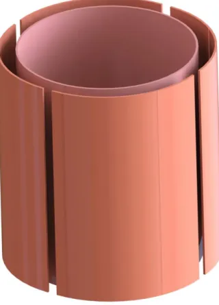
Figure 1.3 Illustration of a model piezoelectric tube scanner. 4-cylinder-sliced
piezoelectric elements are used for the actuation in x and y coordinates and one concentric cylindrical piezoelectric part for actuation in z direction ... 5
Figure 1.4 Illustration of a model photo detector that consist of four independent
photo-diodes. Individual photo-diodes are marked with different letters.. ... 6
Figure 1.5 A sample AFM illustration with a photodetector, cantilever and piezoelectric
scanner... 7
Figure 1.6 One of the macroscale liquid models built by J. D. Bernal in late 50’s [19].
... 10
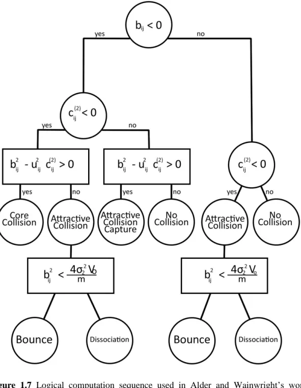
Figure 1.7 Logical computation sequence used in Alder and Wainwright’s work
published in 1959. Image reproduced from the referred paper [22].. ... 12
Figure 1.8 Lennard-Jones interaction between two generic atoms in reduced units. As
can be seen from the figure, when the distance reaches the 1.12σ value, the repulsive part of equation starts to dominate the attractive part and in the distance of σ, the potential energy reaches zero (equilibrium point).. ... 15
xii
Figure 1.9 A flowchart that shows a very basic running algorithm of a MD process..
... 18
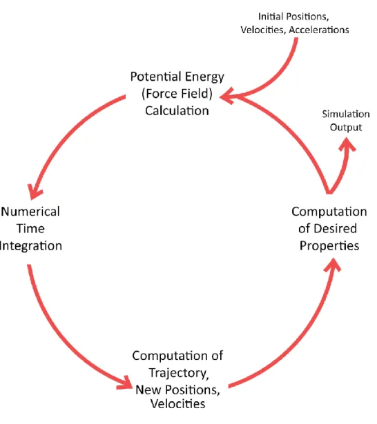
Figure 1.10 Results of protein folding experiments done by Levitt and Warshel. Image
has been reproduced from their 1975 Nature paper [34]. ... 19
Figure 1.11 Image taken from Ye et al.’s work [36]. On the left, three layers of graphene
and silicon dioxide tip can be seen. On the right, there is an additional layer of water molecules between tip and sample.. ... 20
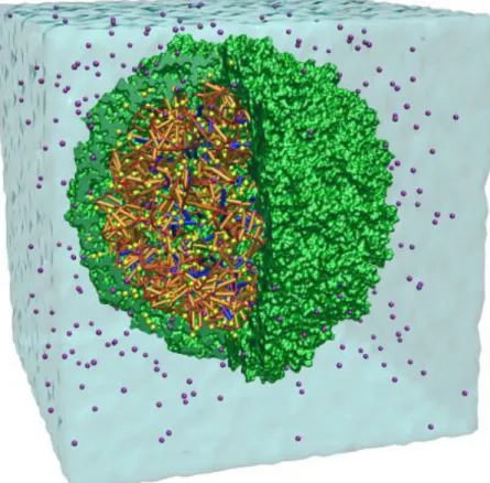
Figure 1.12 MD simulation of a single satellite tobacco mosaic virus in liquid water
environment. The side of the virus capsule is made transparent in order to demonstrate inside of the virus [37]. ... 21
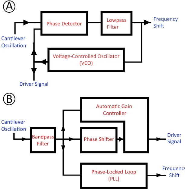
Figure 2.1 (a) Block diagram of a Phase-Locked Loop (PLL). (b) Block diagram of a
typical FM-AFM. Cantilever deflection signal is fed to a bandpass filter in order to filter the noise out. Phase-shifter shifts cantilever response by – π
2 to get the desired phase
difference between input and output. Automatic gain control sets oscillation amplitude to a desired value and PLL provides frequency shift information [41]. ... 24
Figure 2.2 (a) Representative illustration of a cantilever tracking a surface with atomic
resolution. (b) Topography image of the Si (111) surface obtained with the-NC-AFM technique. In unit cell “A”, a misplaced atom (which is a defect) can be seen (34 nm oscillation amplitude and 17 N/m cantilever stiffness) [42]. (c) Topography image of the Sn/Si (111) alloy surface (20 nm oscillation amplitude and 30.5 N/m cantilever stiffness) [44]. (d) Topography image of the KBr (001) surface with a visible step edge (0.15 nm oscillation amplitude and around 1800 N/m cantilever stiffness) [45]. (e) Topography image of C 60 molecules adsorbed on KBr (001) surface (0.15 nm oscillation amplitude and around 1800 N/m cantilever stiffness) [45]. ... 26
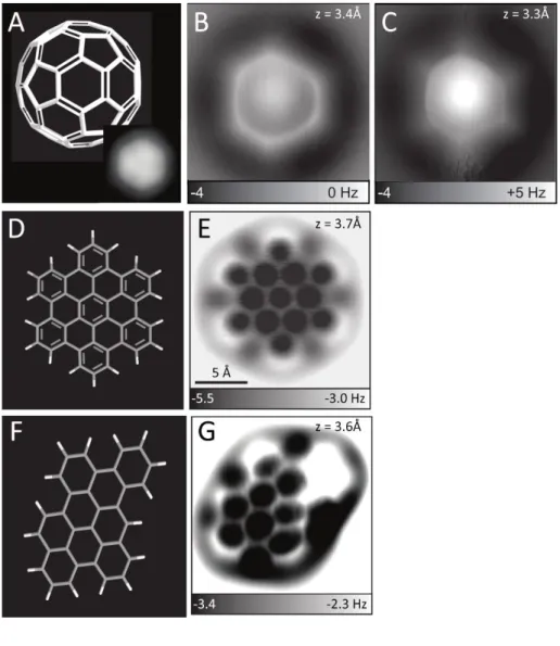
Figure 2.3 (a) Illustration of C 60 molecular model, together with an STM image (b, c)
Constant height NC-AFM measurements of C 60 molecule at different heights. Height is denoted on the images with z. Oscillation amplitude is 0.36 Å. (d) Illustration of Hexabenzocoronene model. (e) Constant height NC-AFM measurements of Hexabenzocoronene molecule. Oscillation amplitude is 0.35 Å. (f) Illustration of DBNP model. (g) Constant height NC-AFM measurements of DBNP molecule. Oscillation amplitude is 0.48 Å. Images reproduced and put together from te work of Gross et al. [46]. ... 28
xiii
Figure 2.4 (a) Illustration of the titanium dioxide (110) surface. (b) “All inclusive”
NC-AFM image of the surface. Color scheme varies with frequency shift. Bridging oxygen atoms are detected as bright spots and titanium atoms form the less bright stripes between them. Both images are reproduced from the work of Bechstein et al. [47]. .. 29
Figure 2.5 (a) Representation of a 3D force field with atomic corrugation. (b) Force
map at 12 pm distance. (c) Force map at 52 pm distance. (d, e) Vertical slices from the 3D force field in (a). (f) Three vertical force curves on two different types of carbon atoms and hollow site on graphite. (g) Energy map at 12 pm distance. (h) Energy map at 52 pm distance. Images are taken from work of Baykara et al. [49]. ... 31
Figure 2.6 (a) Vertical force maps calculated on the NaCl (001) surface with tips of
varying stiffness. Images in (a-d) are calculated alongside the [100] direction and the images in (e-h) alongside the [110] direction. Apparent size changes of attractive and repulsive regions with stiffness can be observed. In color scale, red corresponds to repulsive, blue corresponds to attractive interaction. Image is reproduced from [51]. 33
Figure 2.7 (a-b) Horizontal force maps on obtained bilayer graphene surface with
symmetric and asymmetric tips. Images in (c-d) are vertical force corrugation maps obtained along the white dotted lines in (a-b). Red sites correspond to less attractive regions whereas blue regions corresponds to more attractive regions. Image is reproduced from [52]. ... 34
Figure 2.8 2D version of the tip-sample model used by Pishkenari & Meghdari in their
study. Black spheres represent frozen atoms, orange spheres represent thermostated atoms and yellow spheres represent Newtonian atoms. Image is reproduced from Pishkenari & Meghdari’s work [52]. ... 36
Figure 2.9 NC-AFM scheme used in the work of Nony et al. published in 2006. Image
is reproduced from reference [57].. ... 37
Figure 3.1 Constructed model sample which consists of single layer graphene on top of
bulk platinum. Platinum substrate, single-layer graphene and graphene on platinum can be seen in (a), (b) and (c), respectively.. ... 39
Figure 3.2 Three stages of platinum tip construction. (a) Initial cubic structure. (b)
xiv
Figure 3.3 Side view of the simulated system. Red atoms are fixed, green atoms are
thermostated and blue atoms are free to move. The image of the PacMan ghost represents the interactionless ghost atom that pulls the model tip with a rigid string. 42
Figure 3.4 Block diagram of the NC-AFM model working in constant height mode.
Frequency detection and driving the cantilever are performed by a phase-locked loop. Driving (excitation) signal’s amplitude is modulated with a PI amplitude controller. Interaction force is calculated with respect to the tip-surface distance and applied to the oscillating AFM cantilever.. ... 43
Figure 3.5 Block diagram of the NC-AFM model working in constant height mode.
Frequency detection and driving the cantilever are performed by a phase-locked loop. Driving (excitation) signal’s amplitude is modulated with a PI amplitude controller. Cantilever base – surface distance is modulated according to the difference between the actual frequency shift and a set value. Interaction force is calculated with respect to the tip-surface distance and applied to the oscillating AFM cantilever. ... 45
Figure 4.1 (a) Force map obtained on the graphene surface in “Fixed Surface & Fixed
Tip” configuration at 3 Å separation. (b) Force-distance data over a carbon atom and a hollow site and their interpolated curves. Separation after 3.5 Å distance is highly visible ... 48
Figure 4.2 In (a), the spatial disturbance in the force map due to tip asymmetry is
marked. Two types of carbon atoms are named as A and B, and areas of the same magnitude of forces are enclosed with dashed lines. Two perimeters are projected on one another and the difference between the areas of A and B atoms becomes quite visible. In (b), actual positions of carbon atoms and a hollow site are marked on the force map acquired by the same asymmetric tip. An approximate 0.5 Å of lateral shift in detected positions is observed. ... 49
Figure 4.3 Two force maps obtained in the “Fixed Surface & Free Tip” configuration.
(a) and (b) are taken at separations of 4.5 Å and 4 Å, respectively. There is considerable shift in detected lateral positions of surface sites along both x and y directions. Distortions and artifacts due to atomic motion are visible in (b). ... 51
Figure 4.4 Histogram of tip atom heights (as measured from the tip apex). Free tip
atoms are denoted by blue and fixed tip atoms are denoted by orange. Foremost tip atoms are assumed to have a height of zero before preparation of the histogram. As can
xv
be seen from the histogram, the fixed tip contains more atoms in the near-surface region. The free tip is elongated and contains less atoms in the near-surface region. ... 52
Figure 4.5 (a) Force-distance data over a carbon atom and a hollow site and their
interpolated curves in the “Free Surface & Fixed Tip” configuration. Although separation starts before 3 Å, separation after 3 Å is quite clear. (b) Force map at 2.5 Å separation. The spatial disturbance of the honeycomb structure, caused by tip asymmetry and amplified by surface deformation, is clearly visible. Please note that the indicated tip-sample distances are with respect to the unrelaxed state of the system (i.e., before the graphene moves down to the platinum support by an additional 0.5 Å). ... 53
Figure 4.6 A simulation snapshot from the “Free Surface & Fixed Tip” configuration.
Carbon atoms close to the tip are elevated nearly 0.5Å toward the tip. A white guide line has been drawn under the line of carbon atoms to make elevated atoms more visible. The tip is followed by this bump of carbon atoms like a “Mexican wave”.. ... 54
Figure 4.7 Force maps at (a) 3.5 Å and (b) 4 Å separation obtained in the “Free Surface
& Free Tip” configuration. Although it is very easy to discern the honeycomb structure of the graphene at both tip heights, noise over the force maps due to atomic motion is clearly visible. ... 55
Figure 4.8 Vertical slices of interaction forces obtained via different configurations.
Blue and yellow colored parts represents more and less attractive parts of the surface, respectively. (a) Fixed Surface & Fixed Tip. (b) Fixed Surface & Free Tip. (c) Free Surface & Fixed Tip. (d) Free Surface & Free Tip.. ... 56
Figure 4.9 NC-AFM scans of (a) “Fixed Surface & Fixed Tip” and (b) “Fixed Surface
& Free Tip” configurations in constant height mode. Artifacts discussed for force maps of the configurations are carried over to the scans. Please note that the scan area in (a) is smaller than the horizontal force map presented in Figure 4.1a... 57
Figure 4.10 NC-AFM scans of (a) “Free Surface & Fixed Tip” and (b) “Free Surface
& Free Tip” configurations in constant height mode. Artifacts discussed for force maps of the configurations are carried over to the scans. Please note that the scan area in (a) is smaller than the horizontal force map presented in Figure 4.5b. ... 58
Figure 4.11 NC-AFM constant height mode images taken from the “Free Surface &
xvi
(p-p) oscillation amplitude. (c) Line profiles taken from NC-AFM scans at two different separations of 4.2Å and 4.4Å.. ... 59
Figure 4.12 Constant height scans in the “Free Surface & Free Tip” configuration with
4.2 Å separation and two different p-p oscillation amplitudes: (a) 0.8 Å, (b) 1 Å. As can be seen from the images, increasing the oscillation amplitude decreases the overall frequency shift.. ... 60
Figure 4.13 NC-AFM topography scan of the “Free Surface & Free Tip” configuration
where (a) is the obtained topography map and (b) is the error signal map. Set frequency shift is -222 Hz. Hollow-sites are shown in the topography map with larger heights, in accordance with their higher reactivity when compared with carbon atoms ... 61
Figure 4.14 Two topography scans with (a) -200 Hz and (b) -222 Hz frequency shift
values. With increasing deviation from the initial natural frequency, the corrugation of the topography maps increases, consistent with a smaller mean tip-sample distance. In (b) at the very bottom of the image there are visible artifact due to the less than ideal settings of the distance controller. Please note that the image in (b) has been acquired with different controller parameters than the image in Figure 4.13a. ... 612
Figure 4.15 NC-AFM scan with -220 Hz frequency shift set point, 0.8 Å p-p oscillation
amplitude and a very slow distance controller. (a) Topography map demonstrates very low corrugation (~2 pm) which may be impossible to detect in a real life experiment. (b) Error signal demonstrates very high corrugation in error, when compared with Figure 4.13b... ... 623
Figure 4.16 (a) Topography map obtained with -220 Hz frequency shift set point,
0.8 Å p-p oscillation amplitude and a very fast distance controller. Although corrugation is quite high, it is not easy to distinguish hollow sites of the graphene surface due to controller-induced overall noise over the image. (b) Blue graph demonstrates a line profile taken along the red dashed line in (a). Red line demonstrates the line profile taken from a different scan with a more optimal distance controller. As one can see, very fast controller parameters create additional noise over the physical features rather than improve tracking.. ... 64
1
Chapter 1
1.
Introduction
1.1 Scanning Probe Microscopy
Although atoms have been characterized in many different ways via different physical quantities, “seeing” a single atom was not possible until a new way of microscopy has been invented by Binning et al. in 1981 [1]. Scanning tunneling microscope (STM) is able to get images of surfaces without getting affected by any diffraction limits, because it operates with the principle of “quantum tunneling”. Simply putting a very sharp, metallic probe tip near enough to a surface, optionally with a bias voltage to catalyze the process, makes electrons tunnel between the tip and surface (Figure 1.1). By precisely detecting and locking on the tunneling current between the tip and sample, the topography of the surface can be mapped. STM not only enables researchers to visualize individual atoms and atomic structures, but also provides very vast experimental opportunities. Apart from the ability to see individual atoms; STM provides opportunities to the measurement of spin states [2], standing waves of surface electrons [3], local density of states [4], [5] and many other measurements. In addition STM
2
makes possible the manipulation of surfaces on small length scales, such as the manipulation of individual atoms [6], charges [7] and spins [8]. STM is such a powerful instrument that the inventors of the STM Binnig and Rohrer received the Nobel Prize in Physics in 1986 due to their invention [9]. One can also argue that STM has additional significance in surface science because STM is the first scanning probe microscopy (SPM) technique and other SPM methods with various applications have originated form STM.
Figure 1.1 Illustration of a model surface, a model STM probe tip and tunneling current
(I) flowing between them.
The SPM family of microscopy techniques has started with the STM as discussed above. Their operating principle can be generalized as interaction between a probe and a surface in various ways. As an example, this interaction between surface and the probe may be the tunneling current in STM while it can be the capacitance in scanning capacitance microscopy. There are several SPM techniques that are widely used. Some notable examples are:
Scanning Tunneling Microscopy (STM) Magnetic Force Microscopy (MFM) [10] Scanning Capacitance Microscopy (SCM) [11] Scanning Hall Probe Microscopy (SHPM) [12]
Near-filed Scanning Optical Microscopy (NSOM) [13] Atomic Force Microscopy [14] [15] [16]
3
1.1.1 Basic Principles of SPM
As mentioned above, SPM techniques are based on recording some interaction between a surface to be imaged and a probe. This interaction can be many things depending on the SPM technique, including the tunneling current, force etc. In order to create and detect a desired interaction with the surface, a suitable probe is required. For instance, STM uses (ideally) atomically sharp needle-like tips to measure tunneling current between surface and the probe while NSOM uses a fiber-optic probe to emit and detect light and evanescent field. Although the type of probe may vary (Figure 1.2), a probe to interact with the surface is essential for any SPM operation. Further, this interaction may also be modulated/locked-onto with a feedback control loop. This control mechanism may be very simple or relatively complex depending on the application. But a quick example of SPM probe interaction and feedback can be given from the working mechanism of STM. In STM constant-current mode, the probe position is modulated during scanning in a way to keep the detected tunneling current constant. In a simple overview, the probe gets approached to the surface if tunneling current is less than desired and retracted from the surface if tunneling current is higher than desired In order to be able to scan a surface, or even a line some actuation mechanism is needed to drive the probe across the substrate surface to be scanned. Hence a relative motion in x, y and z coordinates is needed; it does not really matter whether the probe is moved across the surface or the surface moved beneath the probe. In modern SPMs usually this motion is provided by a piezoelectric transducer. Piezoelectric transducers use the piezoelectric effect for actuation of motion. An applied voltage difference to a piezoelectric material results in a strain in the material. In SPM scanners, usually PZT (lead zirconate titanate) type ceramic piezoelectric materials are used. Typical design of a piezoelectric scanner (Figure 1.3) consists of radially polarized arch shaped piezoelectric materials that form together a cylinder. Applying voltage to the independent piezoelectric parts of the cylinder makes those part expand or contract which results in a bending in the overall shape of cylinder that creates a motion in the x and y directions. In addition to these, in order to have an actuation in z direction a concentric cylindrical piezoelectric tube is attached to the system [14].
4
Figure 1.2 Some example SPM probe illustrations; (a) an STM tip, (b) cross-section of
a SNOM tip and (c) an AFM cantilever.
1.1.2 Atomic Force Microscopy
As discussed in the previous section, AFM is a type of scanning probe microscopy invented by none other than the inventor of STM Gerd Binnig and his co-workers in 1986 [15]. In their paper, Binnig remarks that, in order to measure forces in atomic level, they propose to attach the scanning probe tip to a cantilever manufactured by simply gluing a piece of diamond to a thin gold lever, riding it on a sample surface and measuring the resulting deflection of the cantilever with STM. With this setup relying on physical contact rather than the quantum tunneling effect, not only conducting and semiconducting surfaces could be scanned (as is the case for STM), but any surface regardless of its electrical properties. As such, AFM allows topography measurements of any solid surface. It is not far-fetched to say that AFM was and still is a revolutionary instrument. With relatively cheap and simple setups, it is possible to obtain very high resolution topography images, force-distance curves, etc. from nearly any sample.
5
Although the basic idea remained the same, over a brief time period the initial design of AFM changed with more simple, cheap and efficient probes and detection methods which made the instrument more resourceful than ever [16].
Figure 1.3 Illustration of a model piezoelectric tube scanner. 4-cylinder-sliced
piezoelectric elements are used for the actuation in x and y coordinates and one concentric cylindrical piezoelectric part for actuation in z direction.
All typical atomic force microscopes consist of similar parts to operate, although different operation modes may require different electronics or hardware. First of all, since AFM is part of the scanning probe microscopy, AFM needs a probe to operate. A typical AFM uses a very sharp tip (ideally one atom sharp at the end) attached to a micro-machined cantilever which acts as a soft spring to be deflected by tip-sample interaction forces. AFM cantilevers are generally manufactured by using common micro-fabrication techniques like photolithography and etching. Although, cantilevers manufactured can be later coated by many different materials, silicon and silicon nitride are very common materials to manufacture AFM cantilevers from.
6
Figure 1.4 Illustration of a model photo detector that consist of four independent
photo-diodes. Individual photo-diodes are marked with different letters.
As discussed before, AFM detects surface forces by measuring the deflection of the cantilever that holds AFM probe. Although the first AFM used STM for deflection detection, there are many other ways that are being used to measure cantilever deflection (i.e. laser interferometer, capacitive detection). The most common way of measuring cantilever deflection is using a laser and photo detector system. A laser beam reflected onto a photo detector that consist of four independent photo diode (Figure 1.4) can measure very small cantilever deflections. In resting position, the laser reflecting from the cantilever falls in the middle of the photo detector creating no difference in readings of photo diodes. However, any deflection of the cantilever in the normal direction would cause the laser spot to go up or down thus creating a voltage difference between the upper part of the photo detector and its lower part. Therefore a tiny deflection in the cantilever would break the center alignment of the laser spot and hence get detected. Deflection of the cantilever can be quantified with the following equation:
𝜃 = 𝜓 ((𝑉𝐴+ 𝑉𝐵) − (𝑉𝐶+ 𝑉𝐷)) (1.1) where 𝜃 is the deflection of the cantilever, 𝜓 is some calibration constant that correlates voltage to deflection and V values are the voltage readings of photodiodes respective to their sub-indices.
With the described subsystems above, a cantilever with a sharp tip as a scanning probe, an optical detector and a piezoelectric scanner, more or less a very basic AFM can be
7
thought of (see Figure 1.5). Different operation modes of AFM require different types of controller systems and may require additional hardware. For instance; many operating modes of AFM require an oscillating cantilever and thus include a piezoelectric actuator that oscillates the cantilever, while contact mode operation does not require such hardware. Likewise, while a simple tip-sample distance controller is enough for some operating modes, some other operating modes may require more complex controller circuitry. However, the parts discussed above are the basic parts that are common to more or less all AFM designs.
Figure 1.5 A sample AFM illustration with a photodetector, cantilever and piezoelectric
scanner.
AFM can be used in many different operating modes for different purposes. However, the first mode invented was the contact mode. Being the first mode ever invented and the simplest one, contact mode set a basis for the other AFM modes. Yet, since it is still relevant and commonly used, it makes sense to describe the contact mode first. In the contact mode AFM, cantilever and the sample surface are in physical contact in a conventional sense; the tip and the surface are in a repulsive regime of interaction. Due to repulsion between cantilever tip and the surface, the cantilever beam gets deflected
8
in the normal direction. Detecting deflection values during scanning gives quite a good idea about surface topography. This process can be imagined as a blind person reading the Braille alphabet with his fingers. Although this simple mechanism is quite useful for detecting surface topography, it can be damaging to the tip or the sample due to uncontrolled repulsive interaction forces. With the addition of a simple distance controller loop, damage can be significantly reduced. The cantilever base can be approached or retracted from the surface in order to keep a constant set force value, which is directly proportional to the deflection of cantilever. In this method, the cantilever base tracks the sample surface and directly delivers a topography map. The contact mode of AFM is also beneficial in other experiments, for instance the characterization of mechanical properties of the surface. With a well-characterized cantilever, the AFM tip can be pressed into the surface and a force-distance curve can be recorded. With the help of force-distance curves, the elasticity of surfaces can be easily determined. In addition to the surface characterization, contact mode of AFM is widely used in the manipulation of surfaces, characterization of friction, and nanolithography. In addition to its ease and wide range of use, contact mode AFM can also be used in any desired medium like ambient, vacuum and liquid.
Other common modes of the AFM (in addition to contact mode) can be classified as “oscillating modes”. Due to their common use in research; tapping and non-contact modes of the AFM will be introduced in this section. Tapping mode is one of the most widely-used AFM mode available. In this mode, a sinusoidal oscillatory vibration is provided to the cantilever, usually with the help of a piezoelectric actuator at the base of the cantilever mount. Rather than being in contact with the sample constantly, bouncing on top of the sample up and down and “tapping” on it in intermittently yields better results with mechanically delicate samples, such as biological ones. Not having continuous contact with sample and not applying a constant shear force during scanning (as is the case in contact mode) reduces the chance of damaging fragile samples. In addition, tapping mode is also less effected by capillary forces acting under ambient conditions. Under ambient conditions, most surfaces are covered with a very thin water layer. Although this layer usually passes unnoticed in our daily lives, it creates a huge difference in small scales. During contact mode, capillary forces may trap the tip over
9
the surface or mask actual interactions with the sample. Intermittent contact provided by tapping mode also overcomes capillary issues [14].
Non-contact mode of the AFM (NC-AFM), is quite self-explanatory in terms of basic principle. In NC-AFM, a cantilever with an oscillation amplitude smaller than a few nanometers gets very close to the sample surface but never physically touches it. The only interactions between the sample and the tip are relatively small van der Waals and chemical forces in the attractive regime. These weak attractive interactions cause a reduction of the effective resonance frequency of the cantilever which can be detected and locked on to. Since NC-AFM detects weak interatomic interactions, the main use of the NC-AFM is in getting true atomic-resolution images of surfaces and detecting interatomic and intermolecular forces. This delicate process is usually conducted under vacuum in order to achieve best resolution with high quality factors and to reduce the chance of “blunting” the tip apex via contact with the sample surfaces through capillary forces.
1.2 Molecular Dynamics
Molecular Dynamics (MD) is the study of physical movements, behaviors and interactions between atoms and molecules. Usually, atomic interactions between atoms and molecules are calculated from their potentials and trajectory of the atoms in the systems are determined by solving Newton’s equations of motion by various numerical methods. Predicting, interpreting and experimenting with complex atomic structures with many bodies provides essential benefits to chemistry, physics, biology and many other fields. With MD techniques, the behavior of molecules, their shape and size; near other molecules or in other environments and under different temperature conditions can be examined and predicted with accurate, quantitative results. MD simulations are quite popular due to their flexibility and success at predicting molecular structure and thermodynamic properties of molecular systems [17]. The significance of MD simulations and work is also recognized by the Nobel Prize. In 2013 Karplus, Levitt and Warshel received a Nobel Prize in chemistry for their work in “development of multiscale models for complex chemical systems” which includes MD approaches [18].
10
Figure 1.6 One of the macroscale liquid models built by J. D. Bernal in late 50’s [19].
Even before the widespread usage of computers in academia, MD-like simulation ideas were in researchers’ minds and the building of macroscopic models of atoms and molecules were done by researchers. For instance, Bernal investigated the structure of liquids and neighboring atoms in liquids using rubber balls and sticks (see Figure 1.6) in his work published in Nature in 1959 [19]. In his paper, Bernal mentions the first MD works happening in the very same years and states his hopes regarding the adaptation of his work to computing machines used by Alder and Wainwrights. Bernal later mentions his macroscale liquid models and their challenges in his Bakerian Lecture in 1962 as: “… I took a number of rubber balls and stuck them together with rods of a selection of different relative lengths ranging from 2.75 to 4 in. I tried to do this in the first place as casually as possible, working in my own office, being interrupted every five minutes or so and not remembering what I had done before the interruption.” [20]. It can be said that MD as a valid scientific technique started in the beginning due to the work of Alder and Wainwright in late 50’s [21], [22] which are also mentioned by Bernal in that time. In their work, Alder and Wainwright simulated atoms as perfectly
11
elastic hard spheres and modeled their collusions (see Figure 1.7). They extracted thermodynamic and dynamic properties of molecules from their model. After initial steps, MD developed fairly fast and started to spread more. There are some notable works just after Alder and Wainwright’s work that developed more different and refined approaches. Work of Gibson et al. from 1960 that examines dynamics of radiation damage by a simulation of a copper block with the Born-Mayer potential model can be given as one of the earliest examples [23]. Later in 60’s Rahman and Verlet published two famous papers in the area which are both using the Lennard-Jones potential. In 1964 Rahman published his study on dynamics and self-diffusion of liquid argon atoms which correlate quite well with experimental results [24]. In 1967, Verlet published his paper on fluidic and thermodynamic properties of argon atoms [25]. This paper is also quite significant because Verlet’s time integration algorithm which is frequently used even today, is introduced in this paper.
MD is a resourceful tool to investigate physical movements, behaviors and interactions between atoms and molecules. From the introduction of the concept to today, it is commonly used by itself as a study of physics or with experiments to provide a better understanding of underlying sources and causes that yield experimental results. Regardless of the area, MD is a powerful and a resourceful tool that can show different probable structures and interactions of molecules in any environmental condition which may not be easily (or ever) achieved in a controlled laboratory environment.
12
Figure 1.7 Logical computation sequence used in Alder and Wainwright’s work
published in 1959. Image reproduced from the referred paper [22].
1.2.1 Basic Principles of MD
Majority of molecular dynamics work can be considered in the scope of classical mechanics that relies on Newton’s equations for motion and the assumptions that let individual atoms to be treated with Newton’s equations of motion. First of these
13
assumptions can be stated as the “Born-Oppenheimer approximation”. In this approximation, electrons of the atom moves instantaneously with movement of the nuclei and nuclear coordinates and trajectory of the atom can be assumed as a systems coordinates. Furthermore, forces acting on the atoms can be expressed with potential energies which only depends on the position of the nuclei. Those potentials can be assumed to involve (i) fairly complex equations to solve, like time-independent version of the Schrödinger’s equation for electronic variables which are used in ab inito MD methods which also considers quantum mechanics and electronic structure of the atoms to build classical/quantum hybrid approaches to treat system with a classical approach and use quantum mechanics to model interactions in small sites, or (ii) fairly simple pre-defined empirical potentials which are commonly used and yield generally successful results [17], [26]. Thinking the atoms as a point masses with no quantum properties but with a potential energy depending on their coordinates gives us freedom to apply Newton’s laws of motion to them. By knowing mass properties of the atoms and deriving forces acting on them from the associated potential energies, their acceleration and hence velocities, momenta and positions can be determined. With this approach, equations of motion of the 𝑖𝑡ℎ atom in an N-atom system can be written with the Newton’s second law:
𝑚𝑖𝑑2𝑟𝑖𝑥 𝑑𝑡2 = − 𝜕𝑈 𝜕𝑟𝑖𝑥, 𝑚𝑖 𝑑2𝑟𝑖𝑦 𝑑𝑡2 = − 𝜕𝑈 𝜕𝑟𝑖𝑦, 𝑚𝑖 𝑑2𝑟𝑖𝑧 𝑑𝑡2 = − 𝜕𝑈 𝜕𝑟𝑖𝑧 (1.2) Where 𝑚𝑖 is the atomic mass, 𝑟𝑖𝑥 𝑟𝑖𝑦 and 𝑟𝑖𝑧 are Cartesian coordinates and U is the atomic potential that is defined according to set system. Hence trajectories of atoms can be calculated. Like any other set pf differential equations, initial conditions of atoms acceleration, velocity and position should be set beforehand.
As mentioned before, many studies of MD use empirical potentials that depend on the position of an atom. Those empirical potentials are also addressed as “force fields” or “interatomic potentials’ in different sources. Those empirical potentials represent quantum-mechanical and chemical interactions between atoms on a simplistic level. Those empirical energy functions are defined to fit with results of experimental data or quantum-mechanical calculations of very small and limited systems. Usually, defined energy functions include atomic charge, radius, bond length, angle and so forth. These
14
interatomic potentials can be investigated under two main headings: pair potentials and many-body potentials. Pair potentials can be described as a function which defines the potential energy between two interacting atoms. A simple example that can be given for pair potentials is the Coulomb potential that results from charge interactions;
𝐸 = 𝐶𝑞𝑖𝑞𝑗
𝑟 (1.3)
Where C is the Coulomb constant, qi and qj are the net charges of interacting atoms and
r is the interatomic distance. As one can see from the Equation 1.3, the interaction between two atoms get stronger as they get closer. If an attractive case is imagined, there is nothing keeping atoms from getting infinitesimally close to each other and forming a black hole or super condensed heavy mass considering only Equation 1.3. However, in real life no such thing happens due to the Pauli repulsion principle. As two atoms get close to each other their electrons in the shell starts to overlap therefore resulting in a very strong net repulsive force [17]. In order to include strong repulsion when atoms get too close to each other some of the researchers, especially in the very early MD work, used the hard sphere model. In the hard sphere model atoms are assumed to have a spherical shape which is allowed by the Born-Oppenheimer approximation. Furthermore, those assumed spherical shapes have rigid walls which are impenetrable. Therefore we can add a repulsive ψ term to the calculated potential which is defined in Equation 1.4 where σ is assumed the rigid sphere diameter and r is the interaction distance.
𝜓(𝑟) = {
∞ ; 𝑟 < σ 0 ; 𝑟 ≥ σ
(1.4)
Although the hard sphere approach is used in many studies and applicable to many cases, most of the pair potentials includes a rapidly increasing repulsive term which mimics the Pauli repulsion principle. Using a potential with a repulsive region term prevents discontinuities in the potential function, as is the case in the hard sphere model. Hence using pair potentials with a repulsive term results in smoother potential-distance graphs. For example, the very commonly used Lennard-Jones potential that consists of two parts as can be seen in Equation 1.5: one attractive term that scales with r -6 and one repulsive term that scales with r -12 (see Figure 1.8).
15 𝐸 = 4𝜀 [(σ 𝑟) 12 − (σ 𝑟) 6 ] (1.5) 𝐸𝑡𝑜𝑡𝑎𝑙 = 𝐸𝐿𝐽 + 𝐸𝐶𝑜𝑢𝑙 (1.6) Furthermore; the two given examples Coulomb and Lennard-Jones potentials also can be combined in necessary cases, as has been done in literature [26], [27] (see Equation 1.6).
Figure 1.8 Lennard-Jones interaction between two generic atoms in reduced units. As
can be seen from the figure, when the distance reaches the 1.12σ value, the repulsive part of equation starts to dominate the attractive part and in the distance of σ, the potential energy reaches zero (equilibrium point).
Many-body potentials are generally used to model chemically bonded or more complex structures like biomolecules. In those potentials, interaction distance is not sufficient to define a potential energy for an atom. In addition, angle bonds, dihedral angle bonds and so forth may be required to successfully define a potential that represents the simulated system. With introduction of angles and dihedrals, chemical bonding of trios,
16
quartets, and quintuples or more atoms may be incorporated to define correct structures. Some potentials may consider a more detailed geometry or may just be a pair potential that also considers a close neighbor third atom [17]. Some of the notable examples of many body potentials are given below.
Embedded Atom Model: Embedded atom model (EAM) is widely used while
modeling metallic structures and metallic alloys. EAM contains a pairwise potential of an atom with neighboring atom and also considers electron cloud density of neighboring atoms. Potential is calculated with the Equation 1.7 where r𝑖𝑗 is the distance between
atom i and j, ϕ𝑖𝑗 is a short range pair potential between atom i and j, ρℎ,𝑖 is the host density which is approximated by the sum of all the neighboring atoms’ atomic densities (see Equation 1.8 where ρ𝑗𝑎 is the contribution from the density of atom j) and finally F is the embedding potential energy which is a function of ρh,i [28], [29].
𝐸𝑡𝑜𝑡 = ∑ 𝐹𝑖 𝑖(ρℎ,𝑖)+1
2∑𝑖,𝑗 ϕ𝑖𝑗(r𝑖𝑗) 𝑖≠𝑗
(1.7)
ρℎ,𝑖 = ∑𝑗(≠𝑖)ρ𝑗𝑎(r𝑖𝑗) (1.8)
Tersoff Potential: Tersoff potential is a pairwise potential with an attractive term that
is affected by the neighboring environment and bond structures which considers multi bodies. In Tersoff potential, the total potential energy of a system and a bond energy are defined as in Equations 1.8 and 1.9 (Etot is total energy, V is bond energy, f𝑅 is repulsive
pair potential, f𝐴 is attractive pair potential, f𝐶 is a smooth cutoff function that stops
calculation after a cutoff to manage computational resources and b𝑖𝑗 is the measure of bond order that is introduced by Tersoff in his 1998 journal paper [30]). Tersoff potential is generally used for silicon, carbon, diamond structures and may be suitable for hydrocarbons [31].
𝐸𝑡𝑜𝑡 = ∑ E𝑖 𝑖 = 1
2∑𝑖≠𝑗V𝑖𝑗 (1.9)
V𝑖𝑗 = f𝐶(r𝑖𝑗)[a𝑖𝑗f𝑅(r𝑖𝑗) + b𝑖𝑗f𝐴(r𝑖𝑗)] (1.10)
Adaptive Intermolecular Reactive Empirical Bond Order: Reactive Empirical
17
developed to model covalent bonds of carbon-carbon interaction and hydrocarbons. However, due to the absence of dispersion and non-bonded repulsion terms; REBO potential is not a good fit for some solid-state materials (like graphene and graphite), some hydrocarbons, liquids and thin films. Therefore in 2000, Stuart proposed some additions to the REBO potential and proposed Adaptive Intermolecular Reactive Empirical Bond Order (AIREBO) which essentially adds the REBO potential to the Lennard-Jones potential (in some cases Morse potential which is called AIREBO-M) and a torsional potential and be written as [32];
𝐸 = 1
2∑ ∑𝑖 𝑗≠𝑖 ⌈𝐸𝐿𝐽+ 𝐸𝑅𝐸𝐵𝑂 + 𝐸𝑡𝑜𝑟𝑠𝑖𝑜𝑛𝑎𝑙⌉ (1.11)
Interatomic potentials are one of the key elements of an MD simulation. There are many different empirical and semi-empirical potentials that have different strengths and weaknesses in different aspects. Therefore choosing a suitable potential for a given study is crucial and choosing an improper model may lead to undesired and unrealistic systems and results.
So far, trajectories of individual atoms and their position-dependent potentials that result in forces have been discussed. Another essential part of MD simulations is the “time integration”. With the time integration, trajectories of the individual atoms and their new potential energies according to their new positions are calculated. The most common way of integrating an MD system is the Verlet time integration method that was proposed in 1967 [25]. The Verlet algorithm can be put on the paper basically as;
𝑟𝑖(𝑡 + ℎ) = 𝑟𝑖(𝑡 − ℎ) + 2𝑟𝑖(𝑡) + 1
𝑚 ∑𝑗≠𝑖𝑓(𝑟𝑖𝑗(𝑡))ℎ
2 (1.12)
Where t is time, h is the time increment, r is the position of the atom, f is the interatomic force and m is the atomic mass.
18
Figure 1.9 A flowchart that shows a very basic running algorithm of a MD process. 1.2.2 Applications of Molecular Dynamics
As discussed before, MD has many applications in various areas of chemistry, physics, biology and so forth. In the beginning, MD work got popular in materials for obvious reasons. Not long after, MD works were applied to biophysics and biochemistry to mostly examine binding sites and structures of proteins. Especially with the-quantum mechanics-combined approach of ab inito MD, it was possible to successfully simulate chemical interaction sites. MD simulations are used on a wide scale, essentially from
19
theoretical physics to biological applications. Some examples in different areas are briefly presented here in order to demonstrate applications of MD and its wide range. As mentioned above, one of the very first journal articles that employs MD was the work done by Alder and Wainwright which investigates phase transition of argon atoms modeled as hard spheres. In their first publications with MD, they published their phase transition predictions with 108 and 32 particles alongside Monte Carlo simulations conducted by their colleagues which agrees with their results [21], [33]. The association and disassociation mechanisms they published in their later work that explains the MD technique they used can be seen in Figure 1.7 [22].
Figure 1.10 Results of protein folding experiments done by Levitt and Warshel. Image
has been reproduced from their 1975 Nature paper [34].
In 1975 Levitt and Warshel (both 2013 Chemistry Nobel Prize Laureates for their MD work) published a paper in Nature about computer simulations of protein folding. In their work they simplified protein chains to be represented by two C atoms and reduced the degree of freedom of amino acid residues to one. They modeled their system’s potential with a simple Lennard-Jones potential. They minimized the potential energy of linked chains in a damped environment and applied thermal vibrations in cycles as minimization process completes [34]. One of their plots showing their results can be seen in Figure 1.9. Their work’s significance not only comes from its accuracy but from
20
the fact that it is one of the first biological works done with MD. Furthermore it should be considered that their work has been done before Tersoff’s work on potentials which yield result better with hydrocarbon structures, and yet got accurate results.
Another example of MD work in a different area is water adsorption and its effects. Hu and Sun examined the disjoining pressure effect in an ultra-thin water film on gold surface [35]. They prepared a gold sandwich with a thin water layer in-between. They modelled their system with using different potential models according to their system’s needs. They used EAM for calculating the potential between their gold walls and TIP4P-Ew model for water-water molecule interactions. They modeled gold-water interactions with Lennard-Jones and Spohr potentials. Their MD work supported the results coming from classic disjoining theory from adhesion and showed that neither out-of-plane nor in-plane ordering of water films has a big impact on disjoining pressure.
MD simulations are also widely used to interpret tribology and friction experiments. For instance Ye et al. investigated load-dependent friction hysteresis on graphene [36]. They modeled a silicon dioxide AFM tip and multi layers of graphene. In addition to vacuum simulation, a water droplet between surfaces also modeled to simulate ambient conditions. In the work, the Tersoff potential was used in tip atoms and AIREBO was used to model graphene layers. TIP4P potential is used to calculate the potential between water molecules. Interaction between tip, graphene, and if present water was modeled with the Lennard-Jones potential. A snapshot from their simulations can be found in Figure 1.11.
Figure 1.11 Image taken from Ye et al.’s work [36]. On the left, three layers of graphene
and silicon dioxide tip can be seen. On the right, there is an additional layer of water molecules between tip and sample.
21
Another fascinating example of MD use in biology involves modeling of a single complete satellite tobacco mosaic virus done by Freddolino et. al. in 2005 [37]. This simulation contained up to 1 million individual atoms and demonstrated the stability of the virus and its core RNA while demonstrating the instability of shell of the virus without its RNA and discussed physical properties of the virus, its assembly and infection mechanism. This work is still one of the MD simulations with the most particles simulated. A snapshot from their work can be found in Figure 12.
Figure 1.12 MD simulation of a single satellite tobacco mosaic virus in liquid water
environment. The side of the virus capsule is made transparent in order to demonstrate inside of the virus [37].
22
Chapter 2
2.
Literature Survey
2.1 Atomic Resolution Force Microscopy
Even the very first imaging work published by the use of the first ever AFM was able to demonstrate 1 Å vertical resolution under ambient conditions in contact mode [15]. Although this is quite enough to detect atomic steps in structures like graphite layers, it is typically not enough to obtain images of single atoms. Furthermore, using the contact mode of the AFM results in strong repulsive forces between the substrate and the tip and as such, has damaging/blunting effects on the tip apex (as mention in Chapter 1) which prevents atomic resolution or reproducible atomic resolution images. Therefore, in order to take atomic resolution AFM images, oscillating modes of the AFM that operate outside of the repulsive region are used [38]. Therefore it can be said that NC-AFM is commonly used for atomic resolution AFM imaging. In Chapter 1, NC-AFM is briefly introduced together with some other operating modes of the AFM. Since NC-AFM is considered in the scope of this thesis for atomic resolution AFM
imaging, in this section it will be examined more thoroughly and some notable NC-AFM studies will be discussed.
23
Reproducible atomic resolution images have been achieved in the non-contact regime with the frequency modulation (FM) method [39]. To understand the physical mechanism behind frequency modulation, first of all dynamics of the cantilever should be investigated. In a simple view, the AFM cantilever can be assumed as a point mass with one degree of freedom with a forced harmonics oscillation (see Figure 2.1) [40]. Therefore we can write the natural frequency of the cantilever and the equation of motion for the cantilever as:
𝑓0 = √ 𝑘𝑒𝑞
𝑚𝑒𝑓𝑓 (2.1) 𝑚𝑒𝑓𝑓𝑧̈(𝑡) + 𝑐𝑧̇(𝑡) + 𝑘𝑒𝑞𝑧(𝑡) = 𝐹𝑖𝑛𝑡(𝑧(𝑡)) + 𝐹𝑒𝑥𝑐(𝑡) (2.2) where z is the deflection of the cantilever from resting point, c is some damping coefficient, 𝐹𝑖𝑛𝑡 is interaction force between AFM tip and substrate which is distance dependent, 𝑘𝑒𝑞 is the equivalent spring constant of the cantilever and 𝐹𝑒𝑥𝑐 is excitation force externally provided to the cantilever, typically via a piezo actuator. Although the cantilever has a natural resonance frequency of 𝑓0 introducing another term that is
dependent on the deflection changes effective spring constant of the system. Therefore the systems’ natural resonance frequency shifts from the cantilever’s natural resonance frequency. With Equation 2.2, when a cantilever is excited in 𝑓0 there will be a phase
difference of 𝜋
2 between input excitation and output response. However, when the
system’s effective natural frequency is changed due to interaction between tip and sample, this phase difference changes to some value other than 𝜋
2. In FM-AFM, the
phase difference between input excitation and the cantilever response is set to 𝜋
2 which
aims to provide an excitation corresponding to the system’s natural frequency. This aim is achieved by using a phase-locked loop (PLL) to detect and control the oscillation of the cantilever (see Figure 2.1). Output of the Voltage-Controlled Oscillator (VCO) component of the PLL generates a clean sinusoidal wave with constant phase shift matching to cantilever response. Therefore, many AFM systems use VCO output to drive the AFM cantilever (see Figure 2.1a). But the AFM cantilever can also be driven with a phase shifter and an automatic gain controller, without using the VCO output (see Figure 2.1b) [41].
24
Figure 2.1 (a) Block diagram of a Phase-Locked Loop (PLL). (b) Block diagram of a
typical FM-AFM. Cantilever deflection signal is fed to a bandpass filter in order to filter the noise out. Phase-shifter shifts cantilever response by −𝝅
𝟐 to get the desired phase
difference between input and output. Automatic gain control sets oscillation amplitude to a desired value and PLL provides frequency shift information [41].
By setting a fixed frequency shift value and changing the obtained frequency shift to bring it to the set value by making the cantilever come closer to or further away from the surface in the z direction during scanning, the cantilever base is made to precisely track the surface. By keeping record of the z position of the cantilever base, atomic resolution topography maps are obtained (see Figure 2.2a). In 1995 Giessibl and
25
Kitamura & Iwatsuki separately managed to obtain atomic resolution images of the silicon (111) surface with the NC-AFM technique as described above [42], [43]. In his work in 1995, Giessibl used a cantilever beam with 17 N/m stiffness & 34 nm oscillation amplitude and scanned a Si (111) surface in ultra-high vacuum (UHV). With this setup Giessibl was able to image the 77 unit cell of the Si (111) surface with its defects (see Figure 2.2b). The image taken was a reproducible image and portions of the image where individual atoms in their unit cell structure and their defects are non-visible are attributed to where the AFM tip got contaminated or lost its sharpness. Over time, the technique has improved greatly. For instance in 2006, Sugimoto et al. imaged the Sn/Si (111) alloy surface with a similar setup (silicon cantilever with 20 nm oscillation amplitude and 30.5 N/m stiffness in UHV environment, see Figure 2.2c) [44]. While imaging with silicon cantilevers, relatively high oscillation amplitudes are preferred for atomic resolution, because large oscillation amplitudes prevent jump-to-contact and possible instabilities [41]. However, using a quartz tuning fork setup with a metallic tip provides small but stable oscillation amplitudes due to high stiffness. Oscillating the tip with a small oscillating amplitude provides more sensitivity to short-range chemical interactions. Therefore, obtaining higher resolutions and getting images of molecules adsorbed on other surfaces is made possible. For instance, with this technique Pawlak et al. investigated C60 molecules adsorbed on the KBr (001) surface [45]. In their work,
KBr surfaces, their step edges and C60 structures on KBr can be clearly seen with a
topography scan (Figure 2.2d,e). They also investigates adsorbed C60 molecules with
constant height mode, which will be discussed later in this chapter. It can be seen that the oscillation amplitude used in their work (0.15 nm) is significantly lower than oscillation amplitudes used by both Giessibl in 1995 (34 nm) or Sugimoto et al. in 2006 (20 nm).
26
Figure 2.2 (a) Representative illustration of a cantilever tracking a surface with atomic
resolution. (b) Topography image of the Si (111) surface obtained with the-NC-AFM technique. In unit cell “A”, a misplaced atom (which is a defect) can be seen (34 nm oscillation amplitude and 17 N/m cantilever stiffness) [42]. (c) Topography image of the Sn/Si (111) alloy surface (20 nm oscillation amplitude and 30.5 N/m cantilever stiffness) [44]. (d) Topography image of the KBr (001) surface with a visible step edge (0.15 nm oscillation amplitude and around 1800 N/m cantilever stiffness) [45]. (e) Topography image of C60 molecules adsorbed on KBr (001) surface (0.15 nm oscillation
27
Obtaining frequency shift data provides information about the interaction force between tip and the surface. By keeping the cantilever base at a constant height, conducting a scan in x & y directions and recording values of frequency shift in positions yields a frequency shift image. Although NC-AFM technique in constant height mode is pretty straight forward and simple, it is used widely to yield successful atomic resolution images of surfaces and even individual molecules. Work done by Gross et al. in 2012 is a good example of high resolution constant height NC-AFM images of single molecules [46]. In their work, Gross et al. took images of several different molecules using NC-AFM images in constant height mode. They were able to measure bond lengths of molecules in their experiments (see Figure 2.3). In the work, Gross et al. functionalized their AFM tip with a CO molecule and took constant height NC-AFM measurements of different molecules that contains carbon-carbon bonds. They demonstrated different bond orders from different molecules. They used fullerenes adsorbed onto the Cu (111) surface, Hexabenzocoronene molecule adsorbed on the Cu (111) surface and dibenzo(cd,n)naphtho(3,2,1,8-pqra)perylene (DBNP) molecules adsorbed on bilayer NaCl which is supported by a Cu(111) surface. Apart from having very high resolution NC-AFM measurements of small molecules, oscillation amplitudes used during the experiments also stands out. Oscillation amplitudes used in the work are lower than a mere 1 Å, down to even one third of 1 Å. As mentioned before, in order to prevent instabilities or the jump-to-contact effect, relatively higher oscillation amplitudes are chosen during typical NC-AFM experiments using relatively soft silicon cantilevers. However, using high stiffness tuning fork systems cantilever instabilities can be overcome and using very low oscillation amplitudes becomes possible. Hence, with lower oscillation amplitudes, the cantilever-surface interaction becomes more sensitive to short range interactions which leads to higher resolution in NC-AFM measurements.
28
Figure 2.3 (a) Illustration of C60 molecular model, together with an STM image (b, c)
Constant height NC-AFM measurements of C60 molecule at different heights. Height is
denoted on the images with z. Oscillation amplitude is 0.36 Å. (d) Illustration of Hexabenzocoronene model. (e) Constant height NC-AFM measurements of Hexabenzocoronene molecule. Oscillation amplitude is 0.35 Å. (f) Illustration of DBNP model. (g) Constant height NC-AFM measurements of DBNP molecule. Oscillation amplitude is 0.48 Å. Images reproduced and put together from the work of Gross et al. [46].
While constant height mode of NC-AFM is quite successful, it has certain disadvantages. One of the most important disadvantage of the constant mode is the lack of a topography tracking mechanism which may cause crashing the tip into the surface or getting away from the surface during the experiments due to, e.g., thermal drift. This


![Figure 1.6 One of the macroscale liquid models built by J. D. Bernal in late 50’s [19]](https://thumb-eu.123doks.com/thumbv2/9libnet/5883511.121499/26.892.262.704.110.562/figure-macroscale-liquid-models-built-j-bernal-late.webp)
![Figure 1.10 Results of protein folding experiments done by Levitt and Warshel. Image has been reproduced from their 1975 Nature paper [34]](https://thumb-eu.123doks.com/thumbv2/9libnet/5883511.121499/35.892.191.778.411.771/figure-results-protein-folding-experiments-levitt-warshel-reproduced.webp)