Journal of Development Economics 38 (1992) 353-370. olland
vector aut
Salim U. Chishti*
AERC. University of Karachi, Pakistan
The Johns Hopkins University, Baltimore MD. USA Acadia University, Wolfr,ille. Nova Scotia, Canada
Bilkent University, Ankara, Turkey
Received February 1990, final version received June 1991
Recent applications of the Vector Autoregression (VAR) technique pioneered by Sims, Litterman and Doan has become popular in macroeconomic modelhug, particularly when knowledge about *true’ structural relations is absent. This study represents the
apply such a technique to Pakistani data for ten key macroeconomic variables.
the earlier studies on Pakistan’s economy our empirical results are intuitive and consts
the predictions of the standard new neoclassical model. More importantly, based on these results, perhaps, one may also shed light on some of the dominant recurring macroecono
Pakistan’s economy.
Government stabillization pollicies p
Correspordence to: Dr.
Wolfville, Nova Scotia BQP
ohsiu K?san Jere
354 S.U. Chishti et al., Macroeconometric modelling arsd Pakistan’s economy
macroeconomic performances of developing economies including Pakistan.
However, there is little known, with authenticity, about the channels through
which changes in these policies percolate throughout the system. A few
studies have attempted to address these issues in Pakistan using both large
and medium size structural models maqvi et al. (1983, 19861, Saqib and
Yasmin (1987), Masood and Ahmed (1980) and Hasan (1987, 19909].
some of these studies have reached contradictory and, at times, even coun
intuitive conclusions depending on the pre-specifications of the structural
relations used.
In the absence of any knowledge about
‘true’relations, the recent
applications of the Vecto.
r Autoregression (VAR) technique pioneered by
Sims (1980, 1982 and 1986) and popularized by Doan et al. (1984;, we
believe, is a possible alternative as this approach seems to be more flexible
than macro modeiiing. As opposed to the
conventional structuralmacroeco-
nomic models, the VAR technique does not require any explicit economic
theory to estimate a model. It also allows one to capture empirical
regularities in the data using fewer key macro variables and thereby
providing insight into channels through which the different policy variables
operate.
Our study represents the
firstattempt to apply such an approach in the
case of Pakistan. In this paper, we develop and estimate an annaul
macroeconometric model for the economy of Pakistan over the period 1960
to 1988 using the innovative VAR technique proposed by Littcrman (1979,
1984) and Sims (1980, 1982 and 1986). The primary focus of this study is to
analyze empirically the strength of short-run and long-run impacts of
anticipated and unanticipated monetary and fiscal policies and external
resources
and
remittances
shocks
(or
innovations)
cs
Pakistan’s
macroeconomy.
The VAR macroeconometric model estimated in this paper includes ten
key macroeconomic variables [i.e., real GDP (RGDP), consumer price index
(P), terms of trade between agriculture and manufacturing sectors (TTAM),
unemployment rate (UEM). real investment (RINI/), real value of remit-
tances (REM), real exports (REXP), real external resources (REXR), money
stock (M) and real government expenditure (RGEX)]. Th:
icipated policy
analysis is conducted using an F-test on the estimated co
ients while the
unanticipated policy shocks are analyzed with impulse response functions
and variance decompositions (VDCs) obtained from the moving-average
representations of the VAR model.
The results of our study include a moderate impact of fist
on monetary expansion, at least in the short run, and a stron
netary expansion o
e organizatiof3
of
tdecompositions. Section 3 ata, el s
It-suits. Concluding remarks a
ar in section
4.In
order to analyze the impact of
targets, a standard complete structural However, such a model can
arbitrary ‘exclusion’
or ‘zero
restrictiovariables in the model. These very inhibit researchers from revising the historical evidence points to such a n are likely to find these exclusion extreme and inflexible. Faced wit recently adopted an alternative
Sims (1984) which uses the modern time series technique known as the vector Autoregression (VAR) method.
The Vector Autoregressive model provides a simple means of explaining or predicting the values of a set of economic variables at any given point in time. VAR is a straightforward, powerful statistical forecasting tee
which can be applied to any set of historical data. Like the structural
the VAR system also generates systems of equations that can project the future paths of economic variables extrapolating from their past historical values. However, the main difference between the VAR s
structural models is that, unlike the structural model, the based entirely on empirical regularities embedded in the data. structural model is tied closely to the economic theory and has to assumptions and the a priori restrictions imposed therein, the V
does not have to resort to the theory per se as, in fact, the data dete~~~es the final system.
Another impor;tsnt issue that the problem of robustness of the researchers [e.g., King (1983), argued that the empirical results fro by changing a model slight1
(1987 and 1989). on the ot paper, however, Todd ( 1990) o
356 S.U. Chishti et al., Ma?r?oeconometric modelling and Pakistan’s
economy
support
broad claims that continue to color general opinions of not
only VAR analyses but also time series analyses in general. (p. 23)
Reconciling both sides of the robustness debate, Todd (1990) further argued:
At the more general level, I again find some truth on each side. I agree
with the critics that many results from VAR models, at least those
constructed with generic macroeconomic variables..
.may in fact not be
robust. However, I also agree with Sims that nonrobustness is not a
general property of VAR results and that even simple VARs can
sometimes provide useful. evidence on economic issues. In short, it is not
generally true that a!! VAR results are robust or that none are. What
does seem true. . . is that researchers using VARs should check their
results for robustness. (p. 20).
In this paper, we have adopted Todd’s suggestion and in the next section
we demonstrate that our estimated results using the VAR approach, to a
reasonable extent, are
robust.2.1.
Estimation procedureAn
nvariable VAR system can be written as
and
A(k)=z-Ale-A,e”-...Amtm,
(3
where x is an
n x1 vector of macroeconomic variables, A is an n x 1 vector
of constants, and U, is an
n x1 vector of random variables, each of which is
serially uncorrelated with constant variance and zero mean,’ Eq. (2) is an
n x nmatrix of normalized polynominai in the lag operator L (ek x = x_ i)
with the first entry of each polynomial on A’s being unity.
Since the error terms (U,) in the above model are serially uncorrelated, a
simple ordinary least squares (OLS) technique would be appropriate to
estimate the model. However, before estimating the parameters of the model
A(&) meaningfully, one must limit the length of the lag in the polynomials. If
+! is the lag length, the number of coefficients to be estimate
where c is the number of constants.
In the VAR model presented above, the current innovations (U,) are
‘The vector of residuals (0,) may not necessarily be conteowever. using the Chnleski decomposition [as su
test for such collinearity of the residuals. We have adopted this ~~~c~du~e to test for
S.V. Chishti et al., Macroecmwmetric modelling and Pakistan’s economy 357 unanticipated but become part of the information set in the next period. This implies that the anticipated impact of a variable is captured in the coefficients of lagged polynomials while the residuals capture unforeseen contemporaneous events. Hence, even though a direct interpretation of the estimated individual coefficients from the VAR system is very difficult [e.g., see Sims ( 1980, p. 20) 3, a joint F-test on these lagged polynomials is,
nevertheless, usefill in providing information regarding the impact of the
anticipaied portion of the right-hand side variables.
In order to analyze the impact of unanticipated policy shocks on the macro variables in a more convenient and comprehensive way, Sims (19$~~ proposed the use of impulse response functions (IRFs) and variance decompositions (VDCs) that are obtained from a moving average represe tation of the VAR model [eqs. (1) and (2)] as shown below:
x=Constant +H,(d)U, (3)
and
H(t)=z-tH,d+H,e+ . . . .
(4)
where 13 is the coefliciaent matrix of the moving averagti rry~W_____-____- -m*p -m-m2Pntatic-m which
can be obtained by successive substitution in eqs. (1) and (2). The elements of the H matrix trace the response over time of a variable i due to a unit shock given to variable j.’ In fact, these impulse response functions will enable us to analyze the dynamic behaviour of the target variables (RGDP, P, T7’.4M,
UEM and RZNI/) due to unanticipated shocks in the policy variables (RGEX or M).
Having derived the variance-covariance from the moving-average rep- resentation, one can then construct the VDCs. VDCs show the port
variance in the prediction for each variable in the system that is attri to its own innovations and to shocks to other variables in the system case, we are most concerned by the portion of the variance
variable(s) that can be explained by shocks to policy variables (
and some other relevant exogenous variables of interest (i.e.,
REM).
358 S.U. Chishti et al., Macroeconometric modeliing and Pakistan’s economy
section 1) that are common to most small macroeconomic models. They are obtained from the Data Bank
of
the AERC Macroeconometric iModeL beiieve that these key macroeconomic variables should cover the small openeconomy and other broader aspects of the economy of Pakistan. All the
variables, except UEM and TTAM, are in natural logarithmic form.4
3.2. Estimation
Choosing lag length. Following oan (1989) and Sims (1980), an appropri-
ate likelihood-ratio test is used to determine the lag length for the VAR model.’ Using the sample period 1%X&1988, and based OG the significance of the Chi-square (x2) value, a lag 1engtIl of two was adopted in this study.
3.3. Results
F-test results. As mentioned earlier, the significance of F-tests on a group of coefflcents estimated using the VAR technique provides a convenient summary for analyzing the impact of the anticipated policies on the target variables. The significance levels of the F-t&s, based on the hypothesis that all lags of a given variable for a particular equation are zero, are reported in table 1. A value of 0.274, for instance, in row 2 and column 11 indicates that the hypothesis of two lagged coefficients of RGDP in the regression equation of M being both equal to zero [i.e., I-IO: /I1 =f12 =0 (based on F-distribution)]
31ndeed. a much larger model with more variables would be desirable and would probably capture the finer details of’ the economy. However, in explaining such a model we may run into serious degrees of freedom problems. For instance, with 10 variables (n) and 2 lags (d), one
would need to estimate 20 (n x t) parameters for each equation. By including just one additional variable into the model the number of parameters to be estimated increases to 22. In addition, if the number of lags is increased by 1, then with the same model the estimated parameters jump to 30.
“In transforming a variable, a natural question arises as to whether one should do an appropriate differencing to identify the stationarity structure of the process. In this context, Doan (198Q) noted that differencing a variable is ‘important’ for at least two reasons in the case of Box-Jenkins ARIMA Modeling: (a) the identification of the stationary structure of the series becomes very difficult using the sample autocorrelation function of the integrated process; (b) when faced with integrated series most of the computer ‘algorithms’ fail in fitting AR1 models. Neither of these concerns, however, is relevant to the VAR models. As a matter of Fuller [(1976, Theorem 85l)j has shown that differencing the data may not produce any gaid so far as the ‘as:Pmptolic efkiency’ of the YAR is concerned ‘even if it is appropriate’. Hn fact, he even argued that differencing a variable ‘throws information away’ while producing no zigkkaat gain. Thus, following Doan (1989) and Fuller (1976), we have avoided differencing our variablcsz
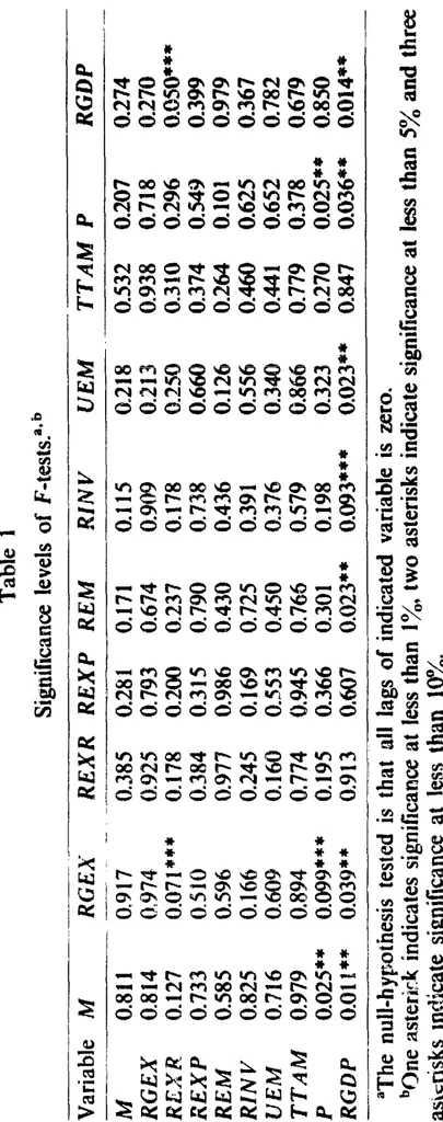
Table 1 Significance levels of F-tests.‘* b
Variable _I-- A4 RGEX REXR REXP REM RIN
V UEM TTAM P RGDP M RGEX REXR (I.811 0.917 0.385 0.814 0,974 0,925 0.127 0.071*** 0.178 0.733 0.510 0.384 0.585 0.596 0.977 0.825 0.166 0.245 0.716 0.609 0.160 0.979 0.894 0.774 0.025** 0.099*** 0.195 0.01 t** 0.039** 0.913 REXP ~.- 0.28 1 0.793 0.200 0.315 0.986 0.169 0.553 0.945 0.366 0.607 REM RINV UEM TTAM P RGDP 0.171 0.115 0.218 0.532 0.207 0.274 0.674 0.909 0.213 0.938 0.718 0.270 0.237 0.178 0.250 0.310 0.296 o.oso*** 0.790 0.738 0.660 0.374 0.549 0.399 0.430 0.436 0.126 0.264 0.101 0.979 0.725 8.391 0.556 0.460 0.625 0.367 0.450 0.376 0.340 0.441 0.652 0.782 0.766 0.579 6.866 0.779 0.378 0.679 0.301 0.198 0.323 0.270 0.025”’ 0.850 0.023* * 0.093*** 0.023** 0.847 0.036** 0.014** “The null-hypothesis tested is that all lags of indicated variable is zero. bCIne asteri& indicates significance at less than lx, two asterisks indicate significance at less than 5% and three asir;risks Indicate significance at less than 10%.
360 S.U. Chishri et al., Macroeconometrk qodelling and Pakistan’s economy
is accepted only 27.4 times out of 100 (or rejected as many as 72.6 times out of loo).
The results in table 1 clearly reveal that the monetary (M) and fiscal (RGEX) policy variables and two other variables of interest i.e., external resources (REXR) and remittances ~~~~) are purely exogenous and they are, in general, not influenced by other variables. This can seen by looking at the significance levei of the relevart ~~.Vcy varia Pes ac~~s$ a given row in table 1. For instance, in the case of RGEX, all v~~u~~ 6
of the F-test (across the ro’“l ..? arle, at least. greater t Table 1 also reveals that the target varia
by the anticipated fiscal IRGEX) and monetary (M) policies and remittances (REM) [significant F-test values in the last row (0.01,
respectively)], while the impact of the external resource ! highly insignificant (0.9 13).
Impulse resp038ses. The results presented, SO far, only enable us to the impact of anticipated policies. Zkthermore, it has been
distributed iag coeficients estimated using VAR do not
understanding of the implied dynamic behaviour of the model. Sims ( 1980),
therefore, suggested the use of impulse response coefficients which will enable us to analyze the dynamic behaviour of a variable due to random shocks given to other variables.’ In fact, the graphs of the impulse response coeflkients provide a better device to analyze the shocks and, therefore, the following &scussion is devoted to the analysis of these graphs.
in order to capture the dynamic efkcts, we considered res onses over five years to a one standard deviation shock in each variable. Si ce the primary
focus of this study is to analyze the impacts of fiscal (RGEX) and monetary (M) policies and, to a lesser extent, the external resources (REXR) and
remittances (REM), we have only presented the graphs of in&se responses to shocks o’ these policy variables and they are shown in fugs. 1, 2, 3 and 4, respectively. The following is a summary tif :he results of im se r~s~onses: la) Inspection of fig. I reveals that a Cine standard deviatio
M produces a strong positive delayed impact on RGDP and takes about two years before reaching a peak.
expansionary phase, the impact of an initial increase in the nominal ba~~~ce~
‘It should be noted that before computing the impulse response functions one should first
orthogonalize the innovations. In this paper, we used the Choleski decom
suggested by Doan (1989), to orthogonalize the variance-covariance matri
It is true that the Choleski decomposition is not unique with respect to the ordering of the
variables except in cases where the VAR covariance matrix is diagonal. Following Sims (1
we have triangularized the system. Based on macro~o~om
of the variables with policy variables zppearin.p, first and
theory, we thed several or&
abHes at %he bA%Orn.
Since varying the order does not s~bsta~tia~~y alter the results. we res f
I 2 3 4 a
-2s
-33
362 S.U. Chishti es al., Macroeconometric modekng and Pakistan’s economy
However, in the long run’ when the nominal money stock is held constant (because of a one period shock) and concurrently prices continuously rising (with lag), the real money balances will start to decline. This is expected to
cause a slowdown in the economy resulting in a decline in real investment, GNP and employment and probably emigration of workers. The emigration of workers may cause an increase in the remittances in the long run.
The results produced by the impulse response function (I F) of ~~~~ are also very interesting and seem to be consistent with the stylized facts of developing countries. The initial impact of the monetary policy (623) on
TTAM* appears to be negative and it is only after a year or so that
TTAM gradually starts to rise. This result seems to support one of t
widely accepted views regarding the thinness of financial markets in the ru or agricultural sector in Pakistan. The short-run impact of M is much weaker on the agricultural prices vis-Lvis the manufacturing prices. ow- ever, with time, the effect of expansionary monetary policy does seem to percoiate through the system and evantualiy the increase in agricultural prices dominates the manufacturing prices.
(b) A one standard deviation shock given to the fiscal variable also produces some interesting results as shown in fig. 2. Unlike monetary policy, the short- run effect of fiscal policy results in a weak response of RGDP and a strong crowding effect on RIWK Concurrently, the general prices (P) tend to decline due to a net increase in the RGDP while the TTAM initiz-uly improves sharply probably due to government expenditure policy programmes. In the long run, however, the support provided by the increased government expenditure (RGEX), in terms of the development of infrastructure, induces
real private investments (RINV) to increase. This increase in RINV conse- quently enhance RGDF and leads to a reduction in the price ievel (P) as ~11 as TTAM. The initial crowding out of RINV seems to generate UEM in the short run as well as in the long run. It is interesting to note that such a result is also produced by the monetary policy.
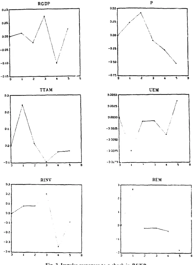
(c) The impulse response functions of external resources (
remittances (REM) produce similar results, at least for RGDP shown in figs. 3 and 4. In both cases, the short-run im
RINV seems to be very subdued. In fact, the results in figs. 3 and 4 seem to support the hypothesis that the role of remittances and external resources has been to stimulate private consumption (thereby causing some increase in
‘Eichenbaum (1985) and others hax cautioned about the reliability of the effects of i:npulse
response functions (IRF) in the long run. The problem arises because in the long ruu the
standard error of llRF tends to be large. Our IRF results may be subject to this caveat and we
caution the reader to view the long run results in such a perspective. We, however, wish to point out that a number of other studies, i.e. Burbidge and Harrison (1984, 1985) ~c~~~~?i~ t.t988), Sims (1980) and others have also analyzed the long run e
‘Note that TTAM is defined as the ratio of prices in the agricultural \estor (A
s
1 a 3 4 5
364 S.U. Chishti et al., Macroeconometric modelling and Pakistan’s economy RCDP oJoy TTAM RINV . P oso, 3.23 /
,,‘“\_
,/’‘\
,/
\
030 /“\
4 .\., -0.2s. \ -0 50“\
. REM IFig. 3. Impulse responses to a shock in REXR.
the money from remittances, at least in the initial stages, is likely to be saved rather than invested in physie21 ca
external resources available and abs t
,, ‘. / ,’ . \ \ .
366 S.U. Chishti et al., Macroeconometric modelbng and Pakistan’s economy
in affecting RGDP and prices in the economy. On the other hand, the external resources and remittances are largely used for consumption and do not sigrificantly influence private investment.
As mentioned earlier, since VDCs can provide further insight into the macroeconomic effects of monetary and fiscal policies, the following discus- sion examines the summary results of VDCs.
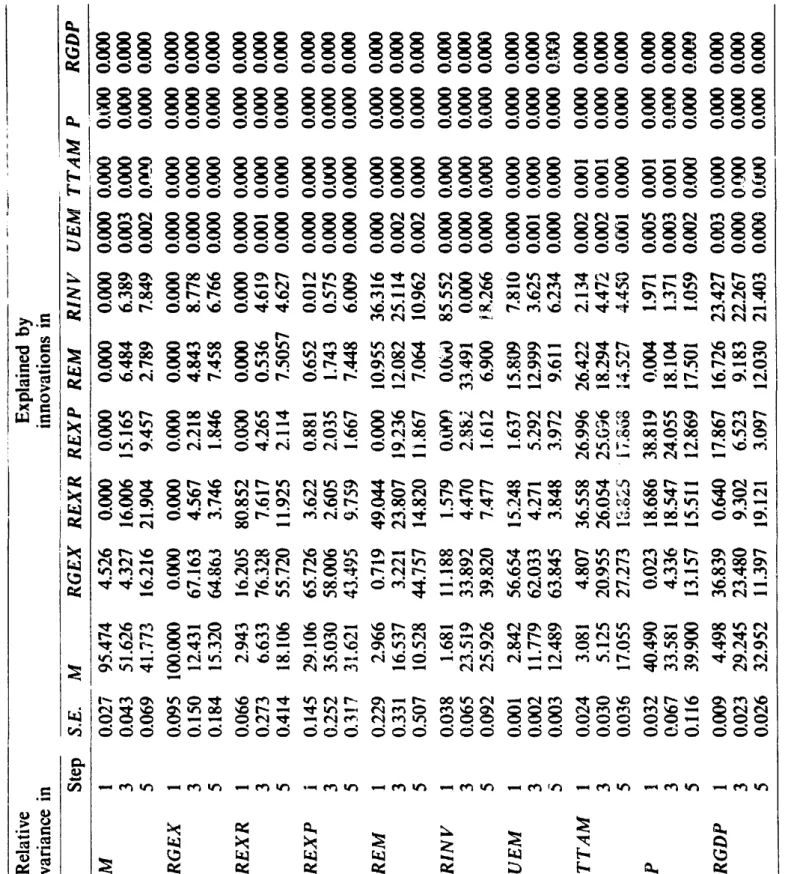
tiriance decompositions (VDCs). The results of the VDCs for all the
variables are reported in table 2. Both direct and indirect effects are captured by the VDCs. Giiven that the main focus of the study is to analyze the impact of monetary and fiscal policies on RGDP we are, therefore, particu- larly interested in that portion of RDGP, which is explained by innovations to M and RGEX. As expected, the direct effects of !ti and RGEX on itself are very high (almost 100’4) and this confirms the exogenous nature of these policy variables. On the other hand, a further analysis of table 2 indicates that a very small portion of the variance in RGDP within a year is explained by innovations to M (4.5%). In fact, innovations to RGEX (36.8x), REXP (17.9”/,), REM (16.7,,, uirre_. “I\ -4 a\,, p ~‘VV (23 4”/*) . explain most df the variation in
RGDP in that time period. However, within three years, innovations to M explain 29.2% of the variance in RGDB whereas innovations to RGEX explain only 23.5% of the variance in RGDB. Innovations to M explain 33.6% of the variance in P after three years while the impact on TTAM has a delayed effect and it goes only up to 27.3% even after five years. It is interesting to note that not only do innovations to RGEX explain a small portion of the variance in RGDP, but such innovations also have a small impact on the other target variable (P). These results seem to be consistent with those of impulse responses.
Robustness qf i/AR results. In order to test the robustness of the estimated VAW results, as suggested by Todd (1990), we compare the results of this paper with that of an earlier comparable study done by Chishti, Hasan and Mahmud (lSS9) [C-H-M (1989) hereafter]. The present model differs from that of the C- -M (1989) study, in at least two important ways: (a) we added two more years of data and (b) an additional variable, TTAM, is also included in the present model. We believe this modification is a significant one and if the present model is nonrobust then, as pointed out by Todd (p. 20, 1990), the results of this study should differ dramatically from that of the C- (1989) model.
Although a co of the results of the two specifications of the V models did not rovide identical results, it is nevertheless, interesting observe that the direction and the overall profile of the present stu
Table 2 Relative variance in Step S.E. M - Summary rew!ts of variance decompositions. __ .~ _ _._-- _^ __ _-- --_- Explained by innovations in .-- __~ RGEX REXR REXP REM RINY VEMi-TTAM P _-. RGDP M 1 3 5 RGEX 1 3 5 REXR 1 3 5 REXP I : REM 1 3 5 RINV 1 3 5 VEM 1 3 5 TTAM 1 3 5 P : 5 RGDP 1 3 5 0.02’7 95.474 4.526 0.000 0.000 0.043 5 1.626 4.327 16.006 15.165 0.069 41.773 16.216 21.904 9.457 0.095 100.000 0.000 0.000 0.000 0.150 12.431 67.163 4.567 2.218 0.184 15.320 64.863 3.746 1.846 0.066 2.943 16.205 80.852 0.W 0.273 6.633 76.328 7.617 4.265 0.414 18.106 55,720 11.925 2.114 0.145 29.106 65.726 3.622 0.881 0.252 35.030 58.006 2.605 2.035 0.317 31.621 43.495 9.759 1.667 0.229 2.966 0.719 49.044 0.000 0.33 1 16.537 3.22 1 23.807 19.236 0.507 10.528 44.757 14.820 1 i .867 0.038 1.681 11.188 1.579 O.iW? 0.065 23.519 33.892 4.470 2.882 0.092 25.926 39.820 7.477 1.612 0.001 2.842 56.654 15.248 1.637 0.002 11.779 62.033 4,271 5.292 0.003 12.489 63.845 3.848 3.972 0.024 3.081 4.807 36.558 26.996 0.030 5.125 20.955 26.054 25.G36 0.036 17.055 27.273 lZ.BLS iY.858 0.032 40.490 0.023 18.686 38.819 0.067 33.581 4.336 18.547 24.055 0.116 39.900 13.157 15.511 12.869 0.009 4.498 36.839 0.640 17.867 0.023 29.245 23.480 9.302 6.523 0.026 32.952 11.397 19.121 3.097
o.ooo
o.ooo
6.484 6.389 2.789 7.849 0.000 0.000 4.843 8.778 7.458 6.766 0.000 0.000 0.536 4.619 7.5057 4.627 0.652 0.012 1.743 0.575 7.448 6.009 10.955 36.316 12.082 25.114 7.064 10.962 0.W 85.552 33.491 0.000 6.900 1 R.266 15.809 7.8 10 12.999 3.625 9.611 6.234 26.422 2.134 f 8.294 4.472 14.527 4.450 0.004 1.971 18.104 1.371 17.501 1.059 16.726 23.427 9.183 22.267 12.030 21.403omo
o.ooo
0.003 o_ooo 0.002 o.wO 0.000 0.000 0.000 0.000 0.000 0.000 0.000 o.ooo 0.001 0.000 0.000 0.000 0.000 0.000 0.000 0.000 0.000 0.000 0.000 0.000 0.002 0.000 0.002 0.000 0.000 o.OuO o.wO 0.000 0.000 0.000 0.000 o.ooo 0.001 0.000 0.000 0.000 0.002 0.001 0.002 0.001 0.001 0.000 0.005 0.001 0.003 0.001 0.002 0.000 0.003 0.000 0.000 0.000 0.000 0.098o.ooo
o.ooo
o.ooo
o.ooo
o.ooo
o.ooo
0.oooo.ooo
o.ooo
omo
oaoo
o.mo
omo
o.ooo
o.ooo
o.ooo
oaoo
o.ooo
omo
omo
o.ooo
o.ooo
omo
o.ooo
o.ooo
0.mo.ooo
o.ooo
o.ooo
o.ooo
o.ooo
0.008o.ooo
o.ooo
o.ooo
o.mo
o.ooo
o.ooo
o.ooo
o.ooo
o.ooo
o.ooo
o.ooo
o.ooo
o.ooo
o.ooo
o.ooo
o.ooo
o.ooo
o.ooo
o.ooo
o.ooo
o.ooo
0400 0.mo.mo
o.ooo
0.mo.uoo
0.mthe results
of t
support the claim that our 5
cyclical behaviaur of the ~~~norny, the
behaviour of the e~~rne~~ af the s
(particularly, in the short run) thaw earlier st
can also be suitable
variables. This study, theref~e, examin
key macrseconomic
policy ~~ar~ab~es
using the innovative VA
( 1979)and Sims
{ 19the economy of Pakistan was est~rn~~
procedure over the period 1960 to 1988.
We believe this p
approach to macro m elling, ~art~c~~ar~y
unknown and ?hat our stu y is the$asg a
in the case of Pakistan. The ern~~r~ca~ results of &hi
intuitive and co~s~st~~t with the
of the stan
(SNN) model,” but based on these results
~rta~t recurring macroec
real sector is still a deb
le issue. Taylor
( ~9~9~~others have theoretically argued in
e proponents of S
theory favoured
empirical resyillts based on the
R approach in
ocks on real GDP seems to be very
370 S.V. Chishti et al., Macroeconometric modelling and Pakistan’s economy
Hasan, M.A., 1990, Phillips curve analysis: Some experiences from Pakistan’s economy, Journal of Economic Studies 17, 57-65.
King, S., 1983, Real interest raies and the interaction of money, output, and prices, Mimeo (Northwestern University, Evanston, IL).
Litter-man, R., 1979, Techniques of forecasting using vector autoregressions, Working paper no. 115 (Federal Reserve Bank of Minneapolis, Minneapolis, MN).
Litterman, R., 1984, Forecasting and policy analysis with bayesian vector autoregression mode%. Federal Researve Bank of Minneapolis Quarterly Review (fall), 30-41.
Masood, K. and E. Ahmed, 1980, The relative importance of autonomous expenditures and money supply in explaining the variations in induced expenditures in the context of Pakistan, Pakistan Economic and Social Review 18, 84-99.
McCallum, B. and 3. Whitaker, 1979, The effectiveness of fiscal feedback rules and automatic stabilizers under rational expectations, Journal of Monetary Economics 5, 171-186.
McMillin, W., 1988, Money grrvth volatility and the macroeconomy, Journal of Money, Credit and Banking 20,319-3X.
Meredith, G., 1989, Expectations, policy shocks, and output behaviour in a multi-country macroeconomic model, Mimeo (Department of Finance, Ottawa, Ont.).
Naqvi, S.N. and A. Ahmed, 1986, The preliminary revised PIDE 1982 macro-econometric model for Pakistan’s economy (PIDE, Islamabad).
Naqvi, S.N., A.H. Khan, N. Khilji and A. Rhmed, 1983, The PIDE macro-eco;u3metric model for Pakistan’s economy (PIDE, Islamabad).
Runkle, D., 1987, Vector autoregression and reality, Journal of Business and Economic Statistics $43742.
Saqib, N. and A. Yasmin, 1987, Some relative evidence on the relative importance of monetary and fiscal policy in Pakistan, Pakistan Development Review 26, 541-549.
Sims, C., 1980, Macroeconomics and reality, Econometrica 48, l-48.
Sims, C., 1982, Policy analysis with econometric models, Brookings Papers on Economic Activity 1, 107-152.
Sims, C., 1986, Are forecasting models usable for policy analysis? Federal Reserve Bank of Minneapolis Quart& Review, Winter, 2-16.
Sims, C., 1987, Comment, Journal of Business alid Economics Statistics 5443-449.
Sims, C., 1989, Models and their uses, American Journal of Agricultural Economics 71.489494. Spencer, D., 1989, Does money matter? the robustness of evidence from vector autoregression,
Journal of Monetary Economics 5, 171-186.
Taylor, J., 1979, Estimation and control of a macroeconomic model with rational expectations, Econometrica 47, 1267-1286.
Taylor, J., 1986, The treatment of expectations in a large multi-country econometric model,, Paper prepared for Brookings Conference on Empirical Macroeconomic for Interdependent Economies, Washington, DC.
Todd, R., 1990, Vector autoregression evidence on monetarism: Another look at the robustness debate, Federal Reserve Bank of Minneapoiis Quarterly Review, Spring, 19-37.