k k
CHAPTER 19
IMPROVING MULTICORE SYSTEM
PERFORMANCE THROUGH DATA
COMPRESSION
Ozcan Ozturk and Mahmut Kandemir
19.1 INTRODUCTION
As applications become more and more complex, it is becoming extremely important to have sufficient compute power on the chip. Multicore and manycore systems have been introduced to address this problem. While multicore system performance and power consumption are greatly affected by application data access characteristics, the compiler optimizations can make a significant difference. Considering that cost of off-chip memory accesses is continuously rising in terms of CPU cycles, it is critical to cut down the number of off-chip memory accesses.
Accessing off-chip memory presents at least three major problems in a multi-core architecture. First, off-chip memory latencies are continuously increasing due to increases in processor clock frequencies. Consequently, large performance penalties are paid even if a small fraction of memory references go off chip. Second, the band-width between the multicore processor and the off-chip memory may not be sufficient to handle simultaneous off-chip access requests coming from multiple processors.
k k
Third, frequent off-chip memory accesses can increase overall power consumption dramatically. Note that power consumption is a critical issue for both embedded sys-tems and large-scale high-performance server platforms.
In order to alleviate these problems, in this chapter we propose an on-chip mem-ory management scheme based on data compression [5]. Our proposal compresses data in memory to (i) reduce access latencies since the compressed data blocks can be accessed faster than the uncompressed blocks; (ii) reduce off-chip bandwidth require-ments since compression can allow on-chip memory to hold more data, cutting the number of off-chip accesses; and (iii) increase the effective on-chip storage capacity. A critical issue in this context however is to schedule compressions and decompres-sions intelligently so that they do not conflict with ongoing application execution. In particular, one needs to decide which processors should participate in the com-pression (and decomcom-pression) activity at any given point during the course of exe-cution. While it is conceivable that all processors can participate in both application execution and compression/decompression activity, this may not necessarily be the best option. This is because in many cases some processors are idle (and therefore cannot take part in application execution anyway) and can be utilized entirely for compression/decompression and related tasks, thereby allowing other processors to focus solely on application execution. Therefore, an execution scheme that carefully
divides the available computing resources between application execution and online
compression/decompression can be very useful in practice.
One might envision two different strategies for such a division: static and dynamic. In the static scheme, the processors are divided into two groups (those performing compression/decompression and those executing the application), and this group-ing is maintained throughout the execution of the application (i.e. it is fixed). In the dynamic scheme, the execution starts with some grouping, but this grouping changes during the course of execution, that is, it adapts itself to the dynamic requirements of the application being executed. This is achieved by keeping track of the wrongly done compressions at runtime and adjusting the number of processors allocated for compression/decompression accordingly. Our main goal in this chapter is to explore these two processor space partitioning strategies, identify their pros and cons and draw conclusions.
We used a set of five array-based benchmark codes to evaluate these two processor partitioning strategies and made extensive experiments with a diverse set of hardware and software parameters. Our experimental results indicate that the most important problem with the static scheme is one of determining the ideal number of processors that need to be allocated for compression/decompression. Our results also show that the dynamic scheme successfully modulates the number of processors used for com-pression/decompression according to the dynamic behavior of the application, and this in turn improves overall performance significantly.
The rest of this chapter is structured as follows: Section 19.2 gives the details of our approach. Section 19.3 presents the results obtained from our experimental analysis. Section 19.4 gives the related work and Section 19.5 describes the future work. Section 19.6 concludes the chapter with a summary of our major observations.
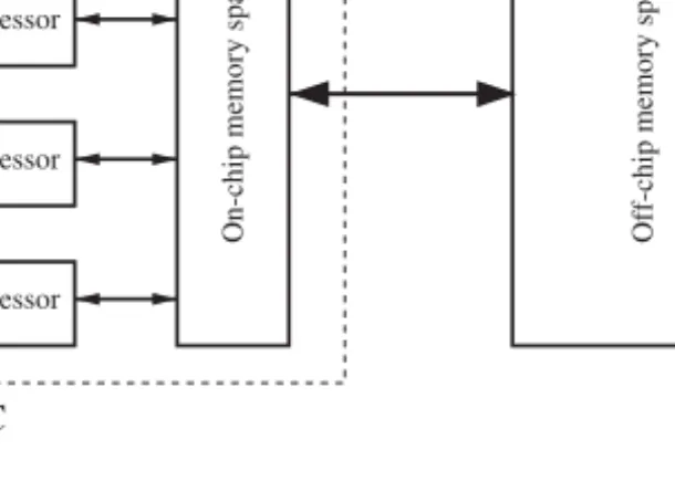
k k OUR APPROACH 387 MPSoC Off-chip m em or y s pace On-chip m em or y s pace Processor Processor Processor Processor
Figure 19.1 The multicore architecture considered in this chapter and the off-chip memory space.
19.2 OUR APPROACH
19.2.1 Architecture and Code Parallelization
The multicore architecture we consider in this chapter is a shared multiprocessor-based system, where a certain number of processors (typically, of the order of 4–32) share the same memory address space. In particular, we assume that there exists an on-chip (software-managed [4, 10, 12, 19]) memory space shared by all processors. We keep the subsequent discussion simple by using a shared bus as the interconnect (though one could use more sophisticated interconnects as well). The processors also share a large off-chip memory space. It should be noted that there is a trend toward designing domain-specific memory architectures [6, 8, 9, 15, 20]. Such architectures are expected to be very successful in some application domains, where the software can analyze the application code, extract the regularity in data access patterns and optimize the data transfers between on-chip and off-chip memories. Such software-managed memory systems can also be more power efficient than a conventional hardware-managed cache-based memory hierarchy [4, 6]. In this study, we assume that the software is in charge of managing the data transfers between the on-chip memory space and the off-chip memory space, though, as will be discussed later, our approach can also be used with a cache-based system. Figure 19.1 shows an example multicore with four parallel processors along with an off-chip storage. We assume that the CPUs can operate only on the data in the on-chip memory.
We employ a loop nest-based code parallelization strategy for executing array-based applications in this multicore architecture. We focus on array-based codes mainly because they appear very frequently in scientific computing domain and embedded image/video processing domain [6]. In this strategy, each loop nest is par-allelized for the coarsest grain of parallelism where the computational load processed by the processors between global synchronization points is maximized. We achieve
k k
this as follows. First, an optimizing compiler (built on top of the SUIF infrastructure [3]) analyzes the application code and identifies all the data reuses and data depen-dences. Then, the loops with data dependences and reuses are placed into the inner positions (in the loop nest being optimized). This ensures that the loop nest exhibits a decent data locality and the loops that remain into the outer positions (in the nest) are mostly dependence-free. After this step, for each loop nest, the outermost loop that does not carry any data dependence is parallelized. Since this type of parallelization tends to minimize the frequency of interprocessor synchronization, we believe that it is very suitable for a multicore architecture. We use this parallelization strategy irrespective of the number of processors used for parallel execution and irrespective of the code version used. It should be emphasized, however, that when some of the processors are reserved for compression/decompression, they do not participate in parallel execution of loop nests. While we use this specific loop parallelization strategy in this work, its selection is actually orthogonal to the focus of this work. In other words, our approach can work with different loop parallelization strategies.
19.2.2 Our Objectives
We can itemize the major objectives of our compression/decompression based on the following on-chip memory management scheme:
• We would like to compress as much data as possible. This is because the more
data are compressed, the more space we have in the on-chip memory available for new data blocks.
• Whenever we access a data block, we prefer to find it in an uncompressed
form. This is because if it is in a compressed form during the access, we need to decompress it (and spend extra execution cycles for that) before the access could take place.
• We do not want the decompressions to come into the critical path of execution.
That is, we do not want to employ costly algorithms at runtime to determine which data blocks to compress, or use complex compression/decompression algorithms.
It is to be noted that some of these objectives conflict with each other. For example, if we aggressively compress each data block (as soon as the current access to it termi-nates), this can lead to a significant increase in the number of cases where we access a data block and find it compressed. Therefore, an acceptable execution model based on data compression and decompression should exploit the trade-offs between these conflicting objectives.
Note that even if we find the data block in the on-chip memory in the compressed form, depending on the processor frequency and the decompression algorithm employed, this option can still be better than not finding it in the on-chip storage at all and bringing it from the off-chip memory. Moreover, our approach tries to take decompressions out of the critical path (by utilizing idle processors) as much as possible, and it thus only compresses the data blocks that will not be needed for some
k k
OUR APPROACH 389
time. Also, the off-chip memory accesses keep getting more and more expensive in terms of processor cycles (as a result of increased clock frequencies) and power consumption. Therefore, one might expect a compression-based multicore memory management scheme to be even more attractive in the future.
19.2.3 Compression/Decompression Policies and Implementation Details
We explore two different strategies, explained below, for dividing the available pro-cessors between compression/decompression (and related activities) and application execution.
• Static Strategy: In this strategy, a fixed number of processors are allocated
for performing compression/decompression activity, and this allocation is not changed during the course of execution. The main advantage of this strategy is that it is easy to implement. Its main drawback is that it does not seem easy to determine the ideal number of processors to be employed for compression and decompression. This is because this number depends on several factors such as the application’s data access pattern, the number of total processors in the multicore and the relative costs of compression and decompression and off-chip memory access. In fact, as will be discussed later in detail, our exper-iments clearly indicate that each application demands a different number of processors (to be allocated for compression/decompression and related activi-ties). Further, it is conceivable that even within an application the ideal number of processors to employ in compression/decompression could vary across the different execution phases.
• Dynamic Strategy: The main idea behind this strategy is to eliminate the
opti-mal processor selection problem of the static approach mentioned above. By changing the number of processors allocated for compression and decompres-sion dynamically, this strategy attempts to adapt the multicore resources to the dynamic application behavior. Its main drawback is the additional overhead it entails over the static one. Specifically, in order to decide how to change the number of processors (allocated for compression and decompression) at run-time, we need a metric that allows us to make this decision during execution. In this chapter, we make use of a metric, referred to as the miscompression rate, which gives the rate between the number of accesses made to the compressed data and the total number of accesses. We want to reduce the miscompression rate as much as possible since a high miscompression rate means that most of data accesses find the data in the compressed form, and this can degrade overall performance by bringing decompressions into the critical path.
Irrespective of whether we are using the static or dynamic strategy, we need to keep track of the accesses to different data blocks to determine their access patterns so that an effective on-chip memory space management can be developed. In our architec-ture, this is done by the processors reserved for compression/decompression. More
k k
specifically, these processors, in addition to performing compressions and decom-pressions, keep track of the past access histories for all data blocks, and based on the statistics they collect, they decide when to compress (or decompress) and when not to. To do this effectively, our execution model works on a data block granular-ity. In this context, a data block is a rectilinear portion of an array, and its size is fixed across the different arrays (for ease of implementation). It represents the unit of
transfer between the off-chip memory and the on-chip memory. Specifically,
when-ever we access a data item that resides in the off-chip memory, the corresponding data block is brought into the on-chip memory (note that this can take several bus cycles). By keeping the size of the data blocks sufficiently large, we can significantly reduce the amount of bookkeeping information that needs to be maintained. A large data block also reduces the frequency of off-chip memory accesses as long as we have a reasonable level of spatial locality.
In more detail, the processors reserved for compression and decompression main-tain reuse information at the data block granularity. For a data block, we define the
interaccess time as the gap (in terms of intervening block accesses) between two
suc-cessive accesses to that block. Our approach predicts the next interaccess time to be the same as the previous one, and this allows us to rank the different blocks accord-ing to their next (estimated) accesses. Then, usaccord-ing this information, we can decide which blocks to compress, which blocks to leave as they are and which blocks to send to off-chip memory. Note that it is possible to use various decision metrics in implementing a compression/decompression scheme, such as usage frequency, last
usage or next usage. In our implementation, we use next usage or interaccess time as
the main criteria for compressions/decompressions. We have also experimented with other metrics, but next usage generates the best results.
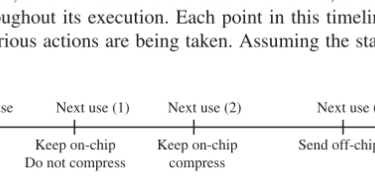
Consider Figure 19.2(a) which depicts the different possible cases for a given data block. In this figure, arrows indicate the execution timeline, that is, the time appli-cation spends throughout its execution. Each point in this timeline is an execution instance where various actions are being taken. Assuming the starting point of this
Next use (3) Next use (2) Next use (1) (b) (a) Decompress (2) Decompress (1) Use Send off-chip Current use Keep on-chip Do not compress Keep on-chip compress
Figure 19.2 (a) Different scenarios for data when its current use is over. (b) Comparison of on-demand decompression and predecompression. Arrows indicate the execution timeline of the program.
k k
OUR APPROACH 391
arrow is indicating the current use of the block, we estimate its next access. If it is soon enough (relative to other on-chip blocks) – denoted Next use (1) – we keep the block in the on-chip memory as it is (i.e. without any compression). On the other hand, if the next access is not that soon (as in the case marked Next use (2)), we com-press it (but still keep it in the on-chip memory). Finally, if the next use of the block is predicted to be really far (see Next use (3) in Fig. 19.2(a)), it is beneficial to send it to the off-chip memory (the block can be compressed before being forwarded to the off-chip memory to reduce transfer time/energy).
Our implementation of this approach is as follows. When the current use of a data block is over, we predict its next use and rank it along with the other on-chip blocks. Then, using two threshold values (Th1and Th2) and taking into account the size (capacity) of the on-chip memory, we decide what to do with the block. More specifically, if the next use of the block is (predicted to be) Tncycles away, we proceed as follows:
• Keep the block in the on-chip memory uncompressed, if Tn≤ Th1, or else
• Keep the block in the on-chip memory compressed, if Th1< Tn≤ Th2, or else
• Send the block to the off-chip memory, if Tn > Th2.
It is to be noted that this strategy clearly tries to keep data with high reuse in on-chip memory as much as possible (even doing so requires compressing the data). As an example, suppose that we have just finished the current access to data block
DBiand the on-chip memory currently holds s data blocks (some of which may be in a compressed form). We first calculate the time for the next use of DBi(call this value
Tn). As explained above, if Tn ≤ Th1, we want to keep DBiin the on-chip memory in an uncompressed form. However, if there is no space for it in the on-chip memory, we select the data block DBjwith the largest next use distance, compress it and forward it to the off-chip memory. We repeat the same procedure if Th1< Tn≤ Th2except that we leave DBiin the on-chip memory in a compressed form. Finally, Tn> Th2, DBi is compressed and forwarded to the off-chip memory. This algorithm is executed after completion of processing any data block. Also, a similar activity takes place when we want to bring a new block from the off-chip memory to the on-chip memory or when we create a new data block.
While this approach takes care of the compression part, we also need to decide when to decompress a data block. Basically, there are at least two ways of handling decompressions. First, if a processor needs to access a data block and finds it in the compressed form, the block should be decompressed first before the access can take place. This is termed as on-demand decompression in this chapter, and an example is shown in Figure 19.2(b) as Decompress (1). In this case, the data block in ques-tion is decompressed just before the access (use) is made. A good memory space management strategy should try to minimize the number of on-demand decompres-sions since they incur performance penalties (i.e. decompression comes in the critical path). The second strategy is referred to as predecompression in this chapter and is based on the idea of decompressing the data block before it is really needed. This is
k k
akin to software-based data prefetching [16] employed by some optimizing compilers (where data is brought into cache memory before it is actually needed for compu-tation). In our implementation, predecompression is performed by the processors allocated for compression/decompression since they have the next access informa-tion for the data blocks. An example predecompression is marked as Decompress (2) in Figure 19.2(b). We want to maximize the number of predecompressions (for the compressed blocks) so that we can hide as much decompression time as pos-sible. Notice that during predecompression the processors allocated for application execution are not affected; that is, they continue with application execution. Only the processors reserved for compression and decompression participate in the predecom-pression activity.
The compression/decompression implementation explained above is valid for both the static and the dynamic schemes. However, in the dynamic strategy case, an addi-tional effort is needed for collecting statistics on the rate between the number of on-demand compressions and the total number of data block accesses (as mentioned earlier, this is called the miscompression rate). Our current implementation maintains a global counter that is updated (within a protected memory region in the on-chip storage) by all the processors reserved for compression/decompression. An impor-tant issue that is to be addressed is when do we need to increase/decrease the number of processors allocated for compression/decompression and related activities. For this, we adopt two thresholds Mr1 and Mr2. If the current miscompression rate is between Mr1and Mr2, we do not change the existing processor allocation. If it is smaller than Mr1, we decrease the number of processors allocated for compression/ decompression. In contrast, if it is larger than Mr2, we increase the number of pro-cessors allocated for compression/decompression. The rationale for this approach is that if the miscompression rate becomes very high, this means that we are not able to decompress data blocks early enough, so we put more processors for decompres-sion. On the other hand, if the miscompression rate becomes very low, we can reduce the resources that we employ for decompression. To be fair in our evaluation, all the
performance data presented in Section 19.3 include these overheads as well.
It is important to measure miscompression rate in a low-cost yet accurate man-ner. One possible implementation is to calculate/check the miscompression rate after every T cycles. Then, the important issue is to select the most appropriate value for T. A small T value may not be able to capture miscompression rate accurately and incurs significant overhead at runtime. In contrast, a large T value does not cause much run-time overhead. However, it may force us to miss some optimization opportunities (by delaying potential useful compressions and/or decompressions). In our experiments, we implemented this approach and also measured the sensitivity of our results to the value of the T parameter. Finally, it should also be mentioned that keeping the access history of the on-chip data blocks requires some extra space. Depending on the value of T, we allocate a certain number of bits per data block and update them each time a data block is accessed. In our implementation, these bits are stored in a certain portion of the on-chip memory, reserved just for this purpose. While this introduces both space and performance overhead, we found that these overheads are not really excessive. In particular, the space overhead was always less than 4%. Also, all the
k k
EXPERIMENTAL EVALUATION 393
performance numbers given in the next section include the cycle overheads incurred for updating these bits.
19.3 EXPERIMENTAL EVALUATION
19.3.1 Setup
We used Simics [18] to simulate an on-chip multiprocessor environment. Simics is a simulation platform for hardware development and design space exploration. It supports modifications to the instruction set architecture (ISA), architectural perfor-mance models and devices. This allows designers to evaluate evolutionary changes to existing systems with a standard software workload. We use a variant of the LZO compression/decompression algorithm [14] to handle compressions and decompres-sions; the decompression rate of this algorithm is about 20 MB/s. It is to be empha-sized that while, in this particular implementation, we chose LZO as our algorithm, our approach can work with any algorithm. In our approach, LZO is executed by the processors reserved for compression/decompression. Table 19.1 lists the base simu-lation parameters used in our experiments. Later in the experiments we change some of these values to conduct a sensitivity analysis.
We tested the effectiveness of our approach using five randomly selected array-based applications from the SpecFP2000 benchmark suite. For each appli-cation, we fast-forwarded the first 500 million instructions and simulated the next 250 million instructions. Two important statistics for these applications are given in Table 19.2. The second column in Table 19.2 (labeled Cycles-1) gives the execution
k k Table 19.2 The benchmark codes used in this study and important statistics.
In obtaining these statistics, the reference input sets are used.
Benchmark Cycles-1 Cycles-2
swim 91,187,018 118,852,504
apsi 96,822,310 127,028,682
fma3d 126,404,189 161,793,882
mgrid 87,091,915 96,611,130
applu 108,839,336 139,955,208
time (in terms of cycles) of the original applications. The values in this column were obtained by using our base configuration (Table 19.1) and using 8 processors to execute each application (without any data compression/decompression). In more details, the results in the second column of this table are obtained using a parallel version of the software-based on-chip memory management scheme proposed in [12]. This scheme is a highly optimized dynamic approach that keeps the most reused data blocks in the on-chip memory as much as possible. In our opinion, it represents the state of the art in software-managed on-chip memory optimization if one does not employ data compression/decompression. The performance (execution cycles) results reported in the next subsection are given as fractions of the values in this second column, that is, they are normalized with respect to the second column of Table 19.2. The third column (named Cycles-2), on the other hand, gives the execution cycles for a compression-based strategy where each processor both participates in the application execution and performs on-demand decompression. In addition, when the current use of a data block ends, it is always compressed and kept on-chip. The on-chip memory space is managed in a fashion which is very similar to that of a full-associative cache. When we compare the results in the last two columns of this table, we see that this naive compression-based strategy is not any better than the case where we do not make use of any compression/decompression at all (the second column of the table). That is, in order to take advantage of data compression, one needs to employ smarter strategies. Our approach goes beyond this simplistic compression-based scheme and involves dividing the processor resources between those that do computation and those that perform compression/decompression-related tasks.
19.3.2 Results with the Base Parameters
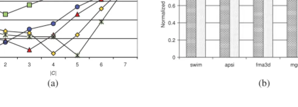
Figure 19.3(a) shows the behavior (normalized execution cycles) of the static approach with different |C| values (|C| = n means n out of 8 processors are used for compression/decompression). As can be seen from the x-axis of this graph, we changed|C| from 1 to 7. One can observe from this graph that in general the different applications prefer different|C| values for the best performance characteristics. For example, while apsi demands 3 processors dedicated for compression/decompression for the best results, the corresponding number for applu is 1. This is because each
k k
EXPERIMENTAL EVALUATION 395
(a) (b)
Figure 19.3 (a) Normalized execution cycles with the static strategy using different|C| values. (b) Comparison of the best static strategy (for each benchmark) and the dynamic strategy.
application has typically a different degree of parallelism in its different execution phases. That is, not all the processors participate in the application execution (e.g. as a result of data dependences or due to load imbalance concerns), and such otherwise idle processors can be employed for compression and decompression. We further observe from this graph that increasing|C| beyond a certain value causes performance deterioration in all applications. This is due to the fact that employing more processors for compression and decompression than necessary prevents the application from exploiting the inherent parallelism in its loop nests, and that in turn hurts the overall performance. In particular, when we allocate 6 processors or more for compression and decompression, the performance of all five applications in our suite becomes worse than the original execution cycles.
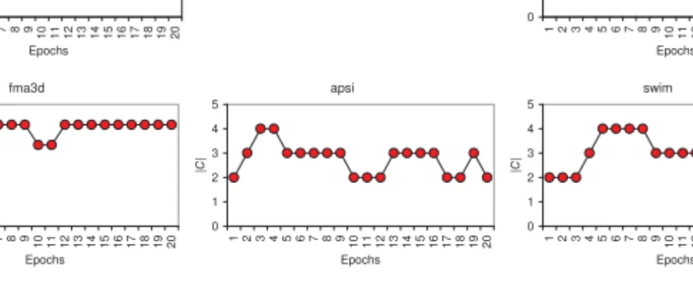
The graph in Figure 19.3(b) gives a comparison of the static and dynamic strate-gies. The first bar for each benchmark in this graph gives the best static version, that is, the one that is obtained using the ideal|C| value for that benchmark. The sec-ond bar represents the normalized execution cycles for the dynamic scheme. One can see from these results that the dynamic strategy outperforms the static one for all five applications tested, and the average performance improvement (across all bench-marks) is about 13.6% and 21.4% for the static and dynamic strategies, respectively. That is, the dynamic approach brings additional benefits over the static one. To better explain why the dynamic approach generates better results than the static one, we give in Figure 19.4 the execution behavior of the dynamic approach. More specif-ically, this graph divides the entire execution time of each application into twenty epochs, and, for each epoch, shows the most frequently used|C| value in that epoch. One can clearly see from the trends in this graph that the dynamic approach changes the number of processors dedicated to compression/decompression over the time, and in this way it successfully adapts the available computing resources to the dynamic execution behavior of the application being executed.
Before moving to the sensitivity analysis part where we vary the default values of some of the simulation parameters, let us present how the overheads incurred by our
k k Figure 19.4 Processor usage for the dynamic strategy over the execution period.
0% 10% 20% 30% 40% 50% 60% 70% 80% 90% 100% Static Dynamic Static Dynamic Static Dynam ic Static Dynam ic Static Dynam ic
swim apsi fma3d mgrid applu
Over
head br
eakdown
Compression Decompression Reuse updates and threshold checks
Figure 19.5 Breakdown of overheads into three different components for the static and dynamic schemes.
approach (effects of which are already captured in Figs 19.3(a) and (b)) are decom-posed into different components. In the bar chart given in Figure 19.5, we give the individual contributions of three main sources of overheads: compression, decom-pression and reuse updates, threshold checks and other bookkeeping activities. We see from these results that, in the static approach case, compression and decompres-sion activities dominate the overheads (most of which are actually hidden during parallel execution). In the dynamic approach case, on the other hand, the overheads are more balanced, since the process of determining the|C| value to be used currently incurs additional overheads. Again, as in the static case, an overwhelming percentage of these overheads are hidden during parallel execution.
k k
EXPERIMENTAL EVALUATION 397
Figure 19.6 Sensitivity of the dynamic strategy to the starting|C| value for the swim bench-mark.
19.3.3 Sensitivity Analysis
In this subsection, we change several parameters in our base configuration (Table 19.1) and measure the variations on the behavior of our approach. Recall that our dynamic approach (whose behavior is compared with the static one in Fig. 19.3(b)) starts execution with |C| = 2. To check whether any other starting value would make a substantial difference, we give in Figure 19.6 the execution profile of swim for the first eight epochs of its execution. One can observe from this graph that no matter what the starting|C| value is, at most after the fifth epoch all execution profiles converge. In other words, the starting|C| value may not be very important for the success of the dynamic scheme except maybe for applications with very short execution times. Although not presented here, we observed a similar behavior with the remaining applications as well. Consequently, playing with the initial value of|C| generated only 3% variance in execution cycles of the dynamic scheme (we omit the detailed results).
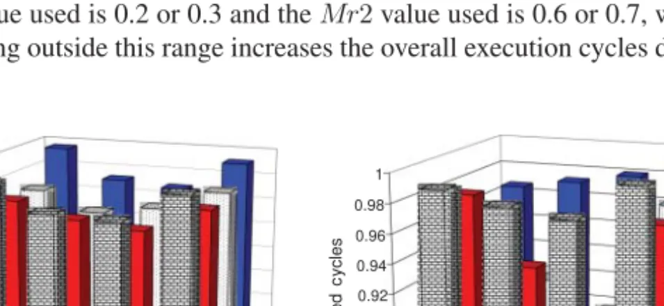
Up to this point in our experimental evaluation we have used the T, Th1, Th2, Mr1 and Mr2 values given in Table 19.1. In our next set of experiments, we modify the values of these parameters to conduct a sensitivity analysis. In Figure 19.7, we present the sensitivity of the dynamic approach to the threshold values Th1 and Th2 for two applications: apsi (a) and mgrid (b). We see that the behavior of apsi is more sensitive to Th2 than to Th1, and in general small Th2 values perform better. This is because a large Th2 value tends to create more competition for the limited on-chip space (as it delays sending data blocks to the off-chip memory), and this in turn reduces the average time that a data block spends in the on-chip memory. However, a very small Th2 value (12,500) leads to lots of data blocks being sent to the off-chip storage prematurely, and this increases the misses in on-chip storage. The other threshold parameter (Th1) also exhibits a similar trend; however, the resulting execution cycles do not range over a large spectrum. This is because it mainly influences the decision of compressing (or not
k k
(a) (b)
Figure 19.7 Sensitivity of the dynamic strategy to T h1, T h2 values. (a) apsi. (b) mgrid.
compressing) a data block, and since compression/decompression costs are lower than that of off-chip memory access (Table 19.1), the impact of Th1 on the behavior of the dynamic scheme is relatively small. Similar observations can be made with the mgrid benchmark as well. This application, however, benefits from a very low
Th2 value mainly because of its poor data locality; that is, once a data block has
been processed, it does not need to be kept on-chip.
The next parameter we study is the miscompression rate thresholds Mr1 and Mr2. Figure 19.8 depicts the normalized execution cycles for two of benchmark codes: apsi (a) and mgrid (b). Our main observation from these graphs is that the best Mr1, Mr2 values are those in the middle of the spectrum experimented. Specifically, as long as the Mr1 value used is 0.2 or 0.3 and the Mr2 value used is 0.6 or 0.7, we are doing fine, but going outside this range increases the overall execution cycles dramatically.
(a) (b)
k k
EXPERIMENTAL EVALUATION 399
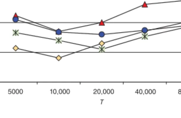
Figure 19.9 Sensitivity of the dynamic strategy to the sampling period (T ).
This can be explained as follows. When the difference between Mr1 and Mr2 is very large, the dynamic scheme becomes very reluctant in changing the value of|C|. As a result, we may miss some important optimization opportunities. In comparison, when the difference between Mr1 and Mr2 is very small, the scheme can make frequent changes to |C| based on (probably) short-term data access behaviors (which may be wrong when considering larger periods). In addition, frequent changes to|C| also require frequent comparisons/checks, which in turn increase the overheads associated with our scheme.
We next study the impact on the effectiveness of the dynamic strategy when the sampling period (T) is modified. The graph in Figure 19.9 indicates that each appli-cation prefers a specific sampling period value to generate the best behavior. For example, the best T value for swim is 10,000 cycles, whereas the best value for fma3d is 20,000. We also observe that working with larger or smaller periods (than this opti-mum one) generates poor results. This is because if the sampling period is very small, we incur a lot of overheads and the decisions we make may be suboptimal (i.e. we may be capturing only the transient patterns and make premature compression and/or decompression decisions). On the other hand, if the sampling period is very large, we can miss opportunities for optimization. While it is also possible to design an adap-tive scheme wherein T is modulated dynamically, it is not clear whether the associated overheads would be negligible.
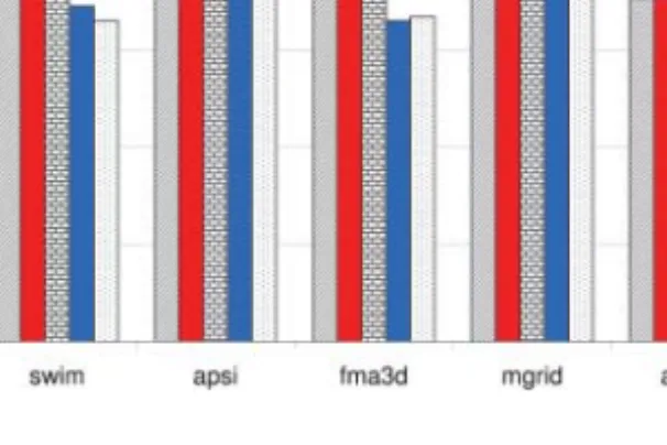
The sensitivity of the dynamic approach to the block size is plotted in Figure 19.10. Recall that block size is the unit of transfer between the on-chip and the off-chip memory, and our default block size was 2 KB. We see from this graph that the aver-age execution cycle improvements with different block sizes range from 18.8% (with 8 KB) to 23.3% (with 1 KB). We also observe that different applications react differ-ently when the block size used is increased. The main reason for this is the intrinsic spatial locality (or block level temporal locality) exhibited by the application. In swim and fma3d, there is a reasonable amount of spatial locality. As a result, these two applications take advantage of the increased block size. In the remaining applica-tions, however, the spatial locality is not as good. This, combined with the fact that
k k Figure 19.10 Sensitivity of the dynamic strategy to the block size.
Figure 19.11 Sensitivity of the static and dynamic strategies to the processor counts.
a small block size allows our approach to manage data space in a finer-granular man-ner, makes a good case for the small block sizes for such applications. Therefore, we witness a reduction in the execution cycles when the data block size is decreased. We next evaluate the impact of the processor count on the behavior of the static and dynamic schemes. Recall that the processor count used so far in our experiments was 8. Figure 19.11 plots the normalized cycles for the best static version and the dynamic version for the benchmark fma3d with different processor counts. An observation that can be made from these results is that the gap between the static and dynamic schemes seems to be widening with increasing number of processors. This is mainly because a larger processor count gives more flexibility to the dynamic approach in allocating resources.
While our focus in this work is on software-managed multicore memories, our approach can work with conventional cache-based memory hierarchies as well. To quantify the impact of our approach under such a cache-based system, we performed
k k RELATED WORK 401 0 0.2 0.4 0.6 0.8 1 1.2
swim apsi fma3d mgrid applu
N
ormalized cycles
Static Dynamic
Figure 19.12 Results with a hardware-based cache memory.
a set of experiments by modeling a 16 KB two-way associative L1 cache for each of the eight processors with a block (line) size of 128 bytes. The results shown in Figure 19.12 indicate that our approach is successful with conventional cache mem-ories as well. The base scheme used (against which the static and dynamic schemes are compared in Fig. 19.12) in these experiments is from [11]. The reason that the savings are not as large as in the software-managed memory case is twofold: First, the unit of transfer between off-chip and on-chip is smaller with the cache-based system (as it is controlled by the hardware). Second, it is more difficult with the cache-based system to catch the stable values for the threshold parameters (Th1, Th2, Mr1 and
Mr2). However, we still observe average 3.1% and 14.8% reductions in execution
cycles due to the static and dynamic schemes, respectively.
19.4 RELATED WORK
Data compression has been investigated as a viable solution in the context of scratchpad memories (SPMs) as well. For example, Ozturk et al. [17] propose a compression-based SPM management. Abali et al. [1] investigate the performance impact of hardware compression. Compression algorithms suitable for use in the context of a compressed cache are presented in [2]. Zhang and Gupta [22] propose compiler-based strategies for reducing leakage energy consumption in instruction and data caches through data compression. Lee et al. [13] use compression in an effort to explore the potential for on-chip cache compression to reduce cache miss rates and miss penalties. Apart from memory subsystems, data compression has also been used to reduce the communication volume. For example, data compression is proposed as a means of reducing communication latency and energy consumption in sensor networks [7]. Xu et al. [21] present energy savings on a handheld device
k k
through data compression. Our work is different from these prior efforts as we give the task of management of the compressed data blocks to the compiler. In decid-ing the data blocks to compress and decompress, our compiler approach exploits the data reuse information extracted from the array accesses in the application source code.
19.5 FUTURE WORK
As has been indicated, there are many parameters that influence the performance of the memory system. In our current implementation, we explore different dimen-sions and different parameters manually. As the next step, we would like to extend our current approach in order to automatically find the most beneficial parameters. Toward this end, we are currently building an optimization framework to handle these parameters in the most effective way.
19.6 CONCLUDING REMARKS
The next-generation parallel architectures are expected to accommodate multiple processors on the same chip. While this makes interprocessor communication less costly (as compared to traditional parallel machines), it also makes it even more crit-ical to cut down the number of off-chip memory accesses. Frequent off-chip accesses do not only increase execution cycles but also increase overall power consumption, which is a critical issue in both high-end parallel servers and embedded systems. One way of attacking this off-chip memory problem in a multicore architecture is to compress data blocks when they are not predicted to be reused soon. Based on this idea, in this chapter, we explored two different approaches: static and dynamic. Our experimental results indicate that the most important problem with static strategies is one of determining the ideal number of processors that need to be allocated for com-pression/decompression. Our results also demonstrate that the dynamic strategy suc-cessfully modulates the number of processors used for compression/decompression according to the needs of the application, and this in turn improves overall perfor-mance. Finally, the experiments with different values of our simulation parameters show that the proposed approach gives consistent results across a wide design space.
REFERENCES
1. B. Abali, M. Banikazemi, X. Shen, H. Franke, D. E. Poff, and T. B. Smith. Hardware compressed main memory: operating system support and performance evaluation. IEEE Transactions on Computers, 50(11):1219–1233, 2001.
2. E. Ahn, S.-M. Yoo, and S.-M. S. Kang. Effective algorithms for cache-level compression. In Proceedings of the 11th Great Lakes symposium on VLSI, pages 89–92, 2001.
k k
REFERENCES 403
3. S. P. Amarasinghe, J. M. Anderson, M. S. Lam, and C. W. Tseng. The SUIF Compiler for Scalable Parallel Machines. In Proc. the Seventh SIAM Conference on Parallel Processing for Scientific Computing, February, 1995.
4. L. Benini, A. Macii, E. Macii, and M. Poncino. Increasing energy efficiency of embed-ded systems by application-specific memory hierarchy generation. IEEE Design & Test of Computers, 17(2): 74–85, April–June, 2000.
5. L. Benini, D. Bruni, A. Macii, and E. Macii. Hardware-assisted data compression for energy minimization in systems with embedded processors. In Proceedings of the DATE’02, Paris, France, March 2002.
6. F. Catthoor, S. Wuytack, E. D. Greef, F. Balasa, L. Nachtergaele, and A. Vandecappelle. Custom Memory Management Methodology – Exploration of Memory Organization for Embedded Multimedia System Design. Kluwer Academic Publishers, June 1998. 7. M. Chen and M. L. Fowler. The importance of data compression for energy efficiency in
sensor networks. In 2003 Conference on Information Sciences and Systems, 2003. 8. CPU12 Reference Manual. Motorola Corporation, 2000. http://motorola.com/
brdata/PDFDB/MICROCONTROLLERS/16_BIT/68HC12_FAMILY/REF_MAT/ CPU12RM.pdf.
9. P. Faraboschi, G. Brown, and J. Fischer. Lx: A technology platform for customizable VLIW embedded processing. In Proceedings of the International Symposium on Computer Architecture, pages 203–213, 2000.
10. M. Kandemir and A. Choudhary. Compiler-directed scratch pad memory hierarchy design and management. In Proceedings of the 39th Design Automation Conference, June 2002. 11. M. Kandemir, A. Choudhary, J. Ramanujam, and P. Banerjee. Improving locality using loop and data transformations in an integrated framework. In Proceedings of the Interna-tional Symposium on Microarchitecture, Dallas, TX, December 1998.
12. M. Kandemir, J. Ramanujam, M. Irwin, N. Vijaykrishnan, I. Kadayif, and A. Parikh. Dynamic management of scratch-pad memory space. In Proceedings of the 38th Design Automation Conference, Las Vegas, NV, June 2001.
13. J. S. Lee, W. K. Hong, and S. D. Kim. Design and evaluation of a selective compressed memory system. In ICCD ’99: Proceedings of the 1999 IEEE International Conference on Computer Design, page 184, 1999.
14. LZO. http://www.oberhumer.com/opensource/lzo/.
15. M-CORE – MMC2001 Reference Manual. Motorola Corporation, 1998. http://www .motorola.com/SPS/MCORE/info_documentation.htm.
16. T. C. Mowry, M. S. Lam, and A. Gupta. Design and evaluation of a compiler algorithm for prefetching. In Proceedings of the 5th International Conference on Architectural Support for Programming Languages and Operating Systems, October 1992.
17. O. Ozturk, M. Kandemir, I. Demirkiran, G. Chen, and M. J. Irwin. Data compression for improving spm behavior. In DAC ’04: Proceedings of the 41st annual conference on Design automation, pages 401–406, 2004.
k k
19. S. Steinke et al. Assigning program and data objects to scratch-pad for energy reduction. In Proceedings of the DATE’02, Paris, France, 2002.
20. TMS370Cx7x 8-bit Microcontroller. Texas Instruments, Revised February 1997. http://www-s.ti.com/sc/psheets/spns034c/spns034c.pdf.
21. R. Xu, Z. Li, C. Wang, and P. Ni. Impact of data compression on energy consumption of wireless-networked handheld devices. In ICDCS ‘03: Proceedings of the 23rd Interna-tional Conference on Distributed Computing Systems, page 302, 2003.
22. Y. Zhang and R. Gupta. Enabling partial cache line prefetching through data compression. In 32nd International Conference on Parallel Processing (ICPP 2003), pages 277–285, 2003.