For Preview Only
Model-based Acceleration Control of Turbofan Engines with a
Hammerstein-Wiener Representation
Jiqiang Wang
a, b, *, Zhifeng Ye
a, Zhongzhi Hu
a, Xin Wu
b, Georgi Dimirovsky
c,
Hong Yue
da. Jiangsu Province Key Laboratory of Aerospace Power Systems, Nanjing University of Aeronautics & Astronautics, Nanjing, Jiangsu Province, 210016, China
b. AVIC Shenyang Engine Design and Research Institute, Shenyang, Liaoning Province, 110015, China c. Dogus University of Istanbul, Istanbul, Turkey
d. The University of Strathclyde, Glasgow, UK
Abstract: Acceleration control of turbofan engines is conventionally designed through either
schedule-based or acceleration-based approach. With the widespread acceptance of model-based design in aviation industry, it becomes necessary to investigate the issues associated with model-based design for acceleration control. In this paper, the challenges for implementing model-based acceleration control are explained; a novel Hammerstein-Wiener representation of engine models is introduced; based on the Hammerstein-Wiener model, a nonlinear generalized minimum variance type of optimal control law is derived; the feature of the proposed approach is that it does not require the inversion operation that usually upsets those nonlinear control techniques. The effectiveness of the proposed control design method is validated through a detailed numerical study.
Keywords: Model-based design; Acceleration control; Nonlinear control; Hammerstein-Wiener
model. 3 4 5 6 7 8 9 10 11 12 13 14 15 16 17 18 19 20 21 22 23 24 25 26 27 28 29 30 31 32 33 34 35 36 37 38 39 40 41 42 43 44 45 46 47 48 49 50 51 52 53 54 55 56 57 58 59 60
For Preview Only
1. Introduction
The concept of model-based design has gained widespread acceptance in many industrial systems. It has transformed how complex systems should be designed, implemented, and tested [1, 2]. Unlike conventional waterfall development model [3], model-based design process can take requirements as part of the model and generate code automatically while carrying out testing and verification continuously [4]. Due to these impressive features, model-based design has embarked on extensive investigation from aviation industry. One of the roadmaps is the model-based control system design for turbofan engines.
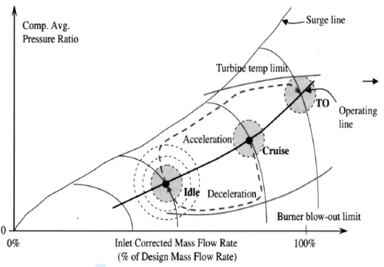
Control of turbofan engines has been a challenging task due to numerous stringent requirements and extreme reliability, particularly with increasing demand arising from complicated tasks such as power management, start logic, takeoff/climbing/cruise control, active clearance and other active controls, engine monitoring and other “intelligent” functions etc. For primary controls, however, turbofan engine control systems are divided functionally into three basic controls: set-point control, transient control and limit protection [5]. Transient control refers to the engine in transient operation when it experiences acceleration or deceleration. The requirement for transient control is therefore to have a safe and fast transient response when manoeuvring. Therefore the optimal operating curve, if plotted on a compressor vs corrected mass flow rate map (see Fig. 1), would be the line following closely the surge line for acceleration and burner blow-out limit for deceleration. In practice, however, enough surge and stability margin should be retained and more importantly, it is extremely challenging to determine where the real surge line locates. This is the reason that transient control is much more challenging to design and accounts for approximately 75% of the total control design and development effort [6].
3 4 5 6 7 8 9 10 11 12 13 14 15 16 17 18 19 20 21 22 23 24 25 26 27 28 29 30 31 32 33 34 35 36 37 38 39 40 41 42 43 44 45 46 47 48 49 50 51 52 53 54 55 56 57 58 59 60
For Preview Only
Fig. 1: Transient control as represented in a compressor vs corrected mass flow rate map
Referring to the above figure, transient control is completed with set point control and transient schedules. That is, acceleration/deceleration process starts from one set point to another set point, and combines with an acceleration/deceleration schedule in between. Therefore issues that should be addressed for transient control include: 1) how to change the engine’s operating condition from one state to another and 2) how to keep the engine from exceeding operating limits while making these state changes (as represented by power lever angle); 3) how to provide acceptable transient performance, e.g. rising time, settling time, overshoot etc. To solve these problems, two approaches are conventionally used: schedule-based transient control and
acceleration-based transient control. In schedule-based transient control, control authority starts
from one set point controller, handles over to the transient controller through a Low-Win logic for acceleration and a High-Win logic for deceleration, before transferring the authority to another set point controller; and the time it takes for the set point controller to hand over the control authority depends on the difference between the beginning and the ending speeds defined by the 3 4 5 6 7 8 9 10 11 12 13 14 15 16 17 18 19 20 21 22 23 24 25 26 27 28 29 30 31 32 33 34 35 36 37 38 39 40 41 42 43 44 45 46 47 48 49 50 51 52 53 54 55 56 57 58 59 60
For Preview Only
deceleration schedules are carefully tuned and this often results in a lookup table embedded into the engine control system logic. This schedule-based control solves the transient control design problem but it may leads to sluggish response and for many situations, the engine is required to have a quick response to power level request. In this case, the acceleration-based transient control can be utilized where the engine produces a desired acceleration or deceleration in engine speed directly, rather than modulate the fuel flow to produce a desired shaft speed.
However, for both schedule-based and acceleration-based controls, it is seen that the key to transient control design is the transient schedule that has been conventionally implemented as lookup tables. These tables are obtained from extensive simulations and experimentations, often resulting in extremely high cost and long development cycle, in addition to the error-prone nature of the trial-and-error methodology. With the wide-spread acceptance of the model-based design concept in aviation industry, it has attracted much attention for the past decades. However there are fundamental difficulties associated with the model-base design for engine transient controls. The reason for this is that the engine dynamics varies significantly over the flight envelope and it is very difficult to obtain a mathematically analytical expression for the engine model. In fact, it is well-known that the aerothermal component-level models can capture the engine dynamics very accurately [7-12]. However the component-level models are not control-oriented due to the fact the key components such as fan, compressor, and turbine are represented by lookup tables or some other non-analytical modules such as (C or Fortran) program codes, while (unfortunately) most of the control theories assume that an analytical model exists before control design. It is illuminating to point out that nonlinear systems theory has developed rapidly over recent decades including concepts such as zero dynamics and normal forms [13], passivity and dissipativity [14], 3 4 5 6 7 8 9 10 11 12 13 14 15 16 17 18 19 20 21 22 23 24 25 26 27 28 29 30 31 32 33 34 35 36 37 38 39 40 41 42 43 44 45 46 47 48 49 50 51 52 53 54 55 56 57 58 59 60
For Preview Only
nonequilibrium theory [15] etc. As a consequence, a number of nonlinear control design techniques have been well established such as feedback linearization [13], recursive designs including backstepping and forwarding [16], energy-based control design for nonholonomic dynamical systems [17] and nonlinear model predictive control [18], to name just a few. However most of the above theories assume implicitly that the system model can be represented by
difference/differential equations. Therefore, for turbofan engines with non-analytical modules, the above methods cannot be applied directly.
To carry out MBD for engine controls, two fundamental approaches can be used to “extract” linear or nonlinear models before the transient control design process. The first one is linearization, however, due to the local nature of linearization techniques, the model such obtained is only valid within a vicinity of certain operating point (usually within 3-5% of engine shaft speed), and this explains the reason that gain scheduling has been universally adopted in aircraft engine control system design, with the most recent development called linear parameter varying control [19-21]. While gain scheduling control has long been a standard practice [22] (particularly for civil aircraft engine controls), its performance may deteriorate seriously during controller switching, and this leads to the development of linear parameter varying (LPV) control to obtain “smooth” transition of controller switching. This LPV approach to MBD of transient control has been extensively investigated in SNECMA [23-28] and the following challenges have been identified: 1) the LPV model of turbofan engines is difficult to obtain; 2) control design is relatively difficult to perform due to the non-convexity of LMI; 3) the order of resulting controllers is relatively high. Therefore LPV modelling and control need further investigation particularly for the benefit of on-board real-time control.
3 4 5 6 7 8 9 10 11 12 13 14 15 16 17 18 19 20 21 22 23 24 25 26 27 28 29 30 31 32 33 34 35 36 37 38 39 40 41 42 43 44 45 46 47 48 49 50 51 52 53 54 55 56 57 58 59 60
For Preview Only
The above difficulties associated with the linearization technique to control-oriented modelling are reflected by the recent trend in utilizing system identification approaches. One of the most often used is the neural networks model that constitutes off-line training and on-line adaptation process to improve accuracy and real-time performance, resulting neural networks models over the flight envelope [29-31]. However, to the best of the authors’ knowledge, there have not been flight-tested results so far. The significance of neural networks, is that it motivates the utilization of other identification methods for on-board real-time modelling and the investigation of control-oriented model-based designs. In this note, a Hammerstein-Wiener representation of the engine transient model is proposed in section 2; for such a model, a generalized minimum variance type of optimal control law is derived in section 3; the feature here is that the proposed control law does not require the inverse operation of the identified nonlinear system model that often troubles many nonlinear control techniques. Section 4 provides a numerical example is to validate the proposed design before the conclusion in section 5.
2. Turbofan Engine Hammerstein-Wiener Modelling
The most accurate engine model is the thermal-mechanical component-level model. This type of models can take heat soakage, time delay, turbine cooling etc into account, hence requiring extensive computing power and relatively long computation time and therefore not suitable for model-based design of transient controls; on the other hand, they are not control oriented since the characteristics of key components such as compressors, combustors, and turbines are given in the form of lookup tables; the presence of such mathematically non-analytical modules prevents the (direct) utilization of most of the control design methodologies. To take care of this situation, as explained above, linearization or identification techniques are utilized. In this paper, an 3 4 5 6 7 8 9 10 11 12 13 14 15 16 17 18 19 20 21 22 23 24 25 26 27 28 29 30 31 32 33 34 35 36 37 38 39 40 41 42 43 44 45 46 47 48 49 50 51 52 53 54 55 56 57 58 59 60
For Preview Only
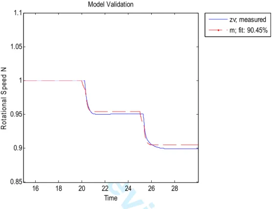
identification approach is taken and a Hammerstein-Wiener representation of the engine model is identified. The result is shown in Fig. 2.
16 18 20 22 24 26 28 0.85 0.9 0.95 1 1.05 1.1 Model Validation Time R ot at io na l S pe ed N zv; measured m; fit: 90.45%
Fig. 2: Hammerstein-Wiener representation of engine model.
The model is obtained with the rotational speed of engine running from 0.9 to 1.0. Considering that a linear model is only valid within 3-5% of the change of rotational speed, the identified Hammerstein-Wiener model retains an acceptable accuracy for 10% of rotational speed change, making it feasible for initial control design evaluation. It is also worth noting that usually there are 6-13 linear models required for interpolation between idle power and TO power. Using nonlinear models may significantly reduce the number of models required and henceforth reduce the switching frequencies. This is advantageous since engine performance can deteriorate during frequent switching. This point has not been fully recognized in engine control system design. 3 4 5 6 7 8 9 10 11 12 13 14 15 16 17 18 19 20 21 22 23 24 25 26 27 28 29 30 31 32 33 34 35 36 37 38 39 40 41 42 43 44 45 46 47 48 49 50 51 52 53 54 55 56 57 58 59 60
For Preview Only
3. Optimal Turbofan Engine Transient Controller Design
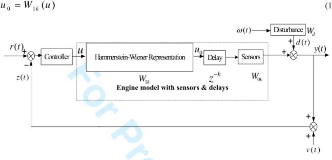
To proceed, for the model above, it can be represented using a nonlinear operator (referring to the following block diagram in Fig. 3):
)
(
1 0W
u
u
k (1) ) (t y ) (t ) (t v Sensors Delay + -+ + + + Controller)
(t
r
) (t z Disturbance k W1z
k W0k d W ) (t du
u
0 Hammerstein-Wiener RepresentationFig. 3: Block diagram of the engine control system
The control system is shown in Fig. 3 where the sensor model W0k is a linear model (usually a first order inertial element). Together with the time delay, the sensor model can be combined with the disturbance model as:
)
(
)
(
)
(
)
(
)
(
)
(
)
1
(
0 0k
t
Du
t
Cx
t
y
t
E
k
t
Bu
t
Ax
t
x
(2)3.1. Optimal controller design
To derive the optimal control signal, a cost function should first be defined. In this paper, the following minimum variance type of index is considered:
0(
t
)
0(
t
)
E
trace
0(
t
)
0(
t
)
E
J
T
T
(3) Engine model with sensors & delays3 4 5 6 7 8 9 10 11 12 13 14 15 16 17 18 19 20 21 22 23 24 25 26 27 28 29 30 31 32 33 34 35 36 37 38 39 40 41 42 43 44 45 46 47 48 49 50 51 52 53 54 55 56 57 58 59 60
For Preview Only
where:
0(
t
)
P
ce
(
t
)
F
cu
(
t
)
, and Pc and Fc are design parameters. Considering the signal delay, the control signal can only affect 0(t) after at least k steps. Therefore there is no loss ofgenerality to expressFcas ck k
c z F
F , then 0(t) can be rewritten as:
(
)
(
)
(
)
(
)
)
(
0
t
k
P
cr
t
k
y
t
k
v
t
k
F
cku
t
(4)Now consider the optimization of the cost function J, the expression J E
0T(t)0(t)
can be represented by a combination of optimal estimation ˆ0(t kt) and estimation error~0(t k t).An application of orthogonality leads to:
0(
t
)
0(
t
)
E
ˆ
0(
t
k
t
)
ˆ
0(
t
k
t
)
E
~
0(
t
k
t
)
~
0(
t
k
t
)
E
J
T
T
T
(5)The estimation error
~0(tkt) is not correlated with control input, henceforth the condition for minimizing the cost function J is that the k-step estimationˆ0(t tk )0.Now:
(ˆ
)
ˆ
(
)
(
)
(
)
)
(
ˆ
0 0t
k
t
P
cr
t
k
t
C
x
t
k
t
Du
t
F
cku
t
(6)In the above equation, for each component:
)
(ˆ
t
k
t
r
: this term is the k-step optimal estimation for reference signal. A reference signal can berepresented by a linear system with disturbance:
)
(
)
(
)
(
)
(
)
1
(
t
x
C
t
r
t
B
t
x
A
t
x
r r r r r r
(7) where:
(t
)
is a white noise with zero mean and unity covariance. Therefore the reference signal k-step optimal estimation is:)
(
)
(ˆ
t
k
t
C
x
t
t
r
r k r
(8) ) ( ˆ t ktx : is the k-step optimal estimation for the combined model, and thus can be written into:
)
(
)
,
(
)
(
ˆ
)
(
ˆ
t
k
t
A
x
t
t
T
0k
z
1Bu
0t
x
k
(9) 3 4 5 6 7 8 9 10 11 12 13 14 15 16 17 18 19 20 21 22 23 24 25 26 27 28 29 30 31 32 33 34 35 36 37 38 39 40 41 42 43 44 45 46 47 48 49 50 51 52 53 54 55 56 57 58 59 60For Preview Only
where: 1 1
1 2 2 ( 1) 1
0
(
k
,
z
)
z
I
z
A
z
A
z
kA
kT
.Now it is required to estimate the state xˆ t(t ). From the well-known Kalman filter theory, the following state estimation equations are obtained:
Predictor:
x
ˆ
(
t
1
t
)
A
x
ˆ
(
t
t
)
Bu
0(
t
k
)
(10) Corrector:x
(ˆ
t
1
t
1
)
x
(ˆ
t
1
t
)
K
f
e
(
t
1
)
e
(ˆ
t
1
t
)
(11))
1
(
ˆ
)
1
(ˆ
)
1
(ˆ
t
t
r
t
t
y
t
t
e
C
rx
r(
t
t
)
C
x
(ˆ
t
1
t
)
Du
0(
t
k
)1
(12) whereKfdenotes the Kalman filter gain matrix.Inserting equation (10) and (12) into (11), and rearranging:
(
)
(
)
(
)
(
)
)
(
)
(ˆ
t
t
T
1z
1e
t
z
1C
x
t
t
T
2z
1u
0t
x
f
r r
f (13) where:
f
f fz
I
I
K
C
Az
K
T
1(
1)
(
)
1 1 (14)
k f f f fz
I
I
K
C
Az
K
D
I
K
C
Bz
z
T
2(
1)
(
)
1 1
(
)
1 (15) The optimal signal uopt(t) that optimizes the cost function J can now be obtained:
C
x
(
t
t
)
CA
x
ˆ
(
t
t
)
CT
0(
k
,
z
1)
B
D
W
1u
(
t
)
F
u
(
t
)
0
P
c rk r k k opt ck opt (16)The optimal condition has the following two alternative representations:
(
,
)
(
)
(ˆ
)
)
(
1 1 1 0k
z
B
D
W
P
C
x
t
t
CA
x
t
t
CT
P
F
t
u
opt
ck
c
k c rk r
k (17) or:
(
)
(ˆ
)
(
,
)
(
)
)
(
1 1 0 1P
C
x
t
t
CA
x
t
t
CT
k
z
B
D
W
u
t
F
t
u
opt
ck c rk r
k
k opt (18)3.2. Optimal controller implementation
Now observe the optimal control signal as generated from equation (17), it requires the inverse operation of the nonlinear engine model, and this is computationally expensive and in many cases infeasible. In fact, for most of the nonlinear control techniques, optimal control solutions are 3 4 5 6 7 8 9 10 11 12 13 14 15 16 17 18 19 20 21 22 23 24 25 26 27 28 29 30 31 32 33 34 35 36 37 38 39 40 41 42 43 44 45 46 47 48 49 50 51 52 53 54 55 56 57 58 59 60
For Preview Only
obtained through the inversion of the nonlinear system, and it is exactly this inversion that hurdles the application of advanced control into practical engineering. Meanwhile the optimal control signal as generated from equation (18) avoids inverse operation of the nonlinear model for its computation, thus it is ideal for real time engine control application. The block diagram for the transient engine control system and controller structure is shown in Fig. 4.
The two parameters Pc and Fck are design freedom to further improve the control performance. Usually, if a PID controller exists that stabilizes the closed loop system, which is the case for most of the civil and military engine controls, experiences show that it is very easy to find a set of Pc and Fck that makes the closed loop stable.
To summarize, the following observations are listed:
(1) Optimal control signal is provided by the state estimator, and therefore it is essentially a Kalman filter based control;
(2) There are two structures for controller implementation. As the latter one does not need the inverse operation of the nonlinear engine model, it is practically appealing for real time engine control;
(3) Two design parameters can be utilized to further improve control performance. Fig. 4: Generation of optimal control signal uopt(t)
) (t y ) (t d ) ( t v ) (t r ) (t z k r
C
) ( tt xr ) ( ˆ tt x kCA
+ + -- + + + + k W1 D B z k CT0( , 1) c ckP
F
1
+ -3 4 5 6 7 8 9 10 11 12 13 14 15 16 17 18 19 20 21 22 23 24 25 26 27 28 29 30 31 32 33 34 35 36 37 38 39 40 41 42 43 44 45 46 47 48 49 50 51 52 53 54 55 56 57 58 59 60For Preview Only
4. Fuel Flow Control of Turbofan Engines for Acceleration: Numerical Study
Now consider the simple case for engine speed closed loop control system: fuel flow control of rotational speed of the engine shaft. The following scenario is assumed: the engine is controlled by fuel flowWf and experiences acceleration from 0.9 to the design point 1.0; it is then decelerated back to 0.9. The Hammerstein-Wiener representation as depicted in section 2 is used for engine model. The two design parameters need to be chosen: first letFck1PI to obtain a stable closed loop control system, where PI denotes the PI controller of the engine; then the parameter Pc is chose to be 1 0.2 -1 0.5 z
Pc . The control performance is shown in Fig. 5, also shown is the corresponding PI control performance.
0 2 4 6 8 10 0.8 0.85 0.9 0.95 1 1.05 1.1 Time (s) R ot at io na l S pe ed (% )
Rotational Speed Tracking
Reference NGMV PI
(a) Acceleration and deceleration performance of the proposed controller, as compared with that of PI control. 3 4 5 6 7 8 9 10 11 12 13 14 15 16 17 18 19 20 21 22 23 24 25 26 27 28 29 30 31 32 33 34 35 36 37 38 39 40 41 42 43 44 45 46 47 48 49 50 51 52 53 54 55 56 57 58 59 60
For Preview Only
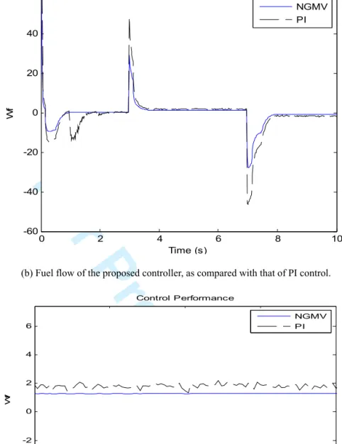
0 2 4 6 8 10 -60 -40 -20 0 20 40 60 Time (s) W f Control Performance NGMV PI(b) Fuel flow of the proposed controller, as compared with that of PI control.
4 4.5 5 5.5 6 -4 -2 0 2 4 6 Time (s) W f Control Performance NGMV PI
(c) Amplified fuel flow curve over 4-6 seconds.
Fig. 5: Closed loop performance while engine accelerates and decelerates between 0.9 and 1.0. It is seen from Fig. 5 that the proposed controller does not significantly improve the performance during engine acceleration and deceleration, but it is still advantageous in the following points:
(1) The transient overshoot is reduced over large envelope flight, and this is shown from the performance during 0-3 seconds. But it is warned that the observed large overshoot is not due to 3 4 5 6 7 8 9 10 11 12 13 14 15 16 17 18 19 20 21 22 23 24 25 26 27 28 29 30 31 32 33 34 35 36 37 38 39 40 41 42 43 44 45 46 47 48 49 50 51 52 53 54 55 56 57 58 59 60
For Preview Only
the PI control design but the model itself. That is, the identified model is not applicable/feasible from idle to 0.9 rotational speed of shaft. However, the proposed controller still suppresses the overshoot effectively;
(2) Fuel consumption is significantly reduced (Fig. 5(b)). Fuel consumption has been a very important performance index for both civil and military engines. It becomes increasingly important for modern engines for clean CO2 emission. In fact, a 1.5% reduction in fuel consumption index is a highly effective design.
(3) Fuel supply becomes much smooth and steady. This is shown in the amplified figure in Fig. 5 (c). Smooth oil supply can reduce the fatigue loss in fuel metering devices, and this can further cut down the fuel consumption. In fact, due to the presence of noises and disturbances in the control loop, the PI controller can amplify the detrimental effects, leading to unsteady control performance. This has been a troubling problem in engine control practice and hardware in the loop testing. In the proposed design, however, the design freedom is chosen to be
1 0.2 -1 0.5 z
Pc , and such a choice improves control performance while providing low-pass filtering effects, resulting in a suppression of noise.
Therefore the simulation results, although still preliminary, have validated the effectiveness of the proposed design. They also provide useful guidance for practical design and lay the foundation for carrying out further research on advanced transient control and hardware in the loop testing.
5. Conclusion
The concept of model-based design has been popularized over the past few years in Chinese aviation industry. Administrational and supervisional architecture have been designed to support the model-based design projects. Meanwhile the enabling technologies in smart sensors, high 3 4 5 6 7 8 9 10 11 12 13 14 15 16 17 18 19 20 21 22 23 24 25 26 27 28 29 30 31 32 33 34 35 36 37 38 39 40 41 42 43 44 45 46 47 48 49 50 51 52 53 54 55 56 57 58 59 60
For Preview Only
response actuators etc have been developed into a readiness level, it is expected that advanced controls including nonlinear control will be applied. In China, however, all of the civil and military engines still use conventional PI control methodology, and no essential research on advanced control is carried out. The development in control theory and control engineering has not been taken advantage of in the field of engine controls. The results presented here, should shed some light on this line of research. Next step of research will focus on the nonlinear control design methodology over large envelope and the corresponding hardware in the loop testing, providing fuel economic demonstration.
Acknowledgements:
We are grateful for the financial support of the Natural Science Foundation of Jiangsu Province (No. BK20140829); Jiangsu Postdoctoral Science Foundation (No.1401017B), and NUAA Fundamental Research Found (No. NS2013020).
References:
[1] Gabriela, N, Mosterman, P.J., eds. Model-Based Design for Embedded Systems. Computational Analysis, Synthesis, and Design of Dynamic Systems 1. Boca Raton: CRC Press, 2010. [2] Reedy, J., Lunzman, S. (2010). Model based design accelerates the development of mechanical
locomotive controls. SAE 2010 Commercial Vehicle Engineering Congress, SAE Technical Paper 2010-01-1999.
[3] McConnell, S. Code Complete, 2nd edition. Microsoft Press, 2004.
[4] Forsberg, K., Mooz, H., Cotterman, H. Visualizing Project Management, 3rd edition, John Wiley and Sons, New York, NY, 2005.
[5] Jaw, L.C., Mattingly, J.D. Aircraft Engine Controls: Design, Systems Analysis, and Health Monitoring, AIAA Inc., Reston, Virginia, 2009.
[6] Jaw, L.C., Garg, S., 2005, Propulsion control technology development in the United States, NASA/TM-2005-213978.
[7] MacIsaak, B.D., Saravanamutto, H.I.H., 1974, A comparison of analog, digital and hybrid computing techniques for simulation of gas turbine performance, ASME Paper No. 74-GT-127. [8] Walsh, P.P., Fletcher, P. Gas Turbine Performance, Blackwell Science, USA, 1998.
[9] Lichtsinder, M., Levy, Y., 2002, Two-sprool, turbo-fan engine: (a) steady-state and dynamic mathematical models, TAE No. 903, Technion, Israel, pp.20-37.
[10] Khalid, S.J., Hearne, R.N., 1980, Enhancing dynamic model fidelity for improved prediction of turbofan engine transient performance, AIAA 80-1083.
[11] Lichtsinder, M., Levy, Y., 2006, Jet engine model for control and real-time simulations, ASME Journal of Engineering for Gas Turbines and Power, 2006, 128: 745-753.
[12] Martin, S., Wallace, I., Bates, D.G., 2008, Development and validation of a civil aircraft engine simulation model for advanced controller design, ASME Journal of Engineering for Gas 3 4 5 6 7 8 9 10 11 12 13 14 15 16 17 18 19 20 21 22 23 24 25 26 27 28 29 30 31 32 33 34 35 36 37 38 39 40 41 42 43 44 45 46 47 48 49 50 51 52 53 54 55 56 57 58 59 60
For Preview Only
Turbines and Power, 2008, 130(5), pp. 051601:1-15.[13] Isidori, A., Nonlinear Control Systems, Springer-Verlag, Berlin, 3rd Edition, 1995.
[14] Van der Shaft, A.J., L2 Gain and Passivity Techniques in Nonlinear Control, Springer-Verlag, Heidelberg, 1996.
[15] Byrnes, C.I., Toward a nonequilibrium theory for nonlinear control systems, in Lecture Notes in Control and Information Sciences, Springer Berlin, 2000.
[16] Sepulchre, R., M. Jankovic and P.V. Kokotovic, Constructive Nonlinear Control, Springer-Verlag, New York, 1997.
[17] Block, A.M., J. Baillieul, P. Crouch and J. Marsden, Nonholonomic Mechanics and Control, Springer, 2003.
[18] Mayne, D.Q., J.B. Rawlings, C.V. Rao and P.O.M. Scokaet, 2000, Constrained model predictive control: stability and optimality, Automatica, 36, 787-814.
[19] Apkarian, P., Gahinet, P., and Becker, G.., 1995, Self-scheduled H∞ control of linear parameter-varying systems: a design example, Automatica, 31, pp. 1251-1261.
[20] Wu, F., Yang, X., Packard, A., Becker, G.., 1996, Induced L2-norm control for LPV systems with bounded parameter variation rates, International Journal of Robust and Nonlinear Control, 6, pp. 983-998.
[21] Stilwell D., and Rugh, W., 2000, Stability preserving interpolation methods for the synthesis of gain scheduled controllers, Automatica, 2000, 36, pp. 665-671.
[22] Prakash, R., Rao, S.V., Skarvan, C.A., 1990, Life enhancement of a gas turbine engine by temperature control, International Journal of Turbo and Jet Engines, 7: 187-206.
[23] Balas, G., 2002, Linear parameter-varying control and its application to a turbofan engine, International Journal of Robust and Nonlinear Control, 12(9): 763-793.
[24] Bruzelius, F. Linear Parameter-varying Systems-an Approach to Gain Scheduling. PhD Thesis, Chalmers University, Göteborg, Sweden, 2004.
[25] Henrion, D., Reberga, L., Bernussou, J., Vary, F., 2004, Linearization and identification of aircraft turbofan engine models, Proceedings of IFAC Symposium on Automatic Control in Aerospace, St. Petersburg, Russia, 2004.
[26] Reberga, L., Henrion, D., Bernussou, J., Vary F., 2005, LPV modeling of a turbofan engine, Proceedings of IFAC World Congress on Automatic Control in Aerospace, Prague, Czech Republic, 2005.
[27] Vary, F., and Reberga, L., 2005, Programming and computing tools for jet engine control design, Proceedings of IFAC World Congress on Automatic Control, Prague, Czech Republic, 2005.
[28] Gilbert, W., Henrion, D., Bernussou, J., Boyer, D., 2010, Polynomial LPV synthesis applied to turbofan engines, Control Engineering Practice, 18: 1077-1083.
[29] Yao, Y., and Sun, J., 2008, Aeroengine direct thrust control based on neural network inverse control, Journal of Propulsion Technology, 29(2), pp. 249-252.
[30] Qi, X., and Fan, D., 2005, Application of improved FSQP algorithm to turbofan engine nonlinear multivariable control, Journal of Propulsion Technology, 26(1), pp. 58-61.
[31] Brunell, B.J., Bitmead, R.R., Connolly, A.J., 2002, Nonlinear model predictive control of an aircrift gas turbine engine, Proceedings of 41st IEEE Conference on Decision and Control, Las Vegas, USA. 3 4 5 6 7 8 9 10 11 12 13 14 15 16 17 18 19 20 21 22 23 24 25 26 27 28 29 30 31 32 33 34 35 36 37 38 39 40 41 42 43 44 45 46 47 48 49 50 51 52 53 54 55 56 57 58 59 60