Classification of agricultural kernels using impact acoustic signal processing

CLASSIFICATION OF AGRICULTURAL

KERNELS USING IMPACT ACOUSTIC

SIGNAL PROCESSING

a thesis

submitted to the department of electrical and

electronics engineering

and the institute of engineering and science

of bilkent university

in partial fulfillment of the requirements

for the degree of

master of science

By

˙Ibrahim ONARAN

February, 2006

I certify that I have read this thesis and that in my opinion it is fully adequate, in scope and in quality, as a thesis for the degree of Master of Science.

Prof. Dr. A. Enis C¸ etin (Supervisor)

I certify that I have read this thesis and that in my opinion it is fully adequate, in scope and in quality, as a thesis for the degree of Master of Science.

Assoc. Prof. Dr. Orhan Arıkan

I certify that I have read this thesis and that in my opinion it is fully adequate, in scope and in quality, as a thesis for the degree of Master of Science.

Assoc. Prof. Dr. U˘gur G¨ud¨ukbay

Approved for the Institute of Engineering and Science:

Prof. Dr. Mehmet B. Baray

Director of the Institute Engineering and Science

ABSTRACT

CLASSIFICATION OF AGRICULTURAL KERNELS

USING IMPACT ACOUSTIC SIGNAL PROCESSING

˙Ibrahim ONARAN

M.S. in Electrical and Electronics Engineering Supervisor: Prof. Dr. A. Enis C¸ etin

February, 2006

The quality is the main factor that directly affects the price for many agricul-tural produces. The quality depends on different properties of the produce. Most important property is associated with health of consumers. Other properties mostly depend on the type of concerned vegetable. For instance, emptiness is im-portant for hazelnuts while openness is crucial for the pistachio nuts. Therefore, the agricultural produces should be separated according to their quality to main-tain the consumers health and increase the price of the produce in international trades. Current approaches are mostly based on invasive chemical analysis of some selected food items or sorting food items according to their color. Although chemical analysis gives the most accurate results, it is impossible to analyze large quantities of food items.

The impact sound signal processing can be used to classify these produces according to their quality. These methods are inexpensive, noninvasive and most of all they can be applied in real-time to process large amount of food. Sev-eral signal processing methods for extracting impact sound features are proposed to classify the produces according to their quality. These methods are includ-ing time and frequency domain methods. Several time and frequency domain methods including Weibull parameters, maximum points and variances in time windows, DFT (Discrete Fourier Transform) coefficients around the maximum spectral points etc. are used to extract the features from the impact sound. In this study, we used hazelnut and wheat kernel impact sounds. The success rate over 90% is achieved for all types produces.

iv

Keywords: Impact sound, Pistachio nuts, Hazelnuts, Wheat kernels, Feature

ex-traction, Classification, Food quality, Aflatoxin, Mel-Cepstrum, Principle Com-ponent Analysis (PCA), Support Vector Machines, Acoustics.

¨

OZET

TARIMSAL ¨

UR ¨

UNLER˙IN C

¸ ARPMA SES˙I

KULLANILARAK SINIFLANDIRILMASI

˙Ibrahim ONARAN

Elektrik ve Elektronik M¨uhendisli˘gi, Y¨uksek Lisans Tez Y¨oneticisi: Prof. Dr. A. Enis C¸ etin

S¸ubat, 2006

Kalite, tarımsal ¨ur¨unlerin fiyatını do˘grudan etkileyen bir fakt¨ord¨ur. ¨Ur¨unlerin kalitesi, bu ¨ur¨unlerin ¸ce¸sitli ¨ozelliklerine ba˘glıdır. Bu ¨ozelliklerin en ¨onemlileri t¨uketicinin sa˘glı˘gıyla ilgili olanlardır. Di˘ger ¨ozellikler genelde ilgilenilen ¨ur¨une ba˘glıdır. Orne˘gin, fındıklar i¸cin bo¸s ya da dolu olması ¨onemliyken, antep¨ fıstıkları i¸cin a¸cık ya da kapalı olması daha ¸cok ¨onemlidir. Tarımsal ¨ur¨unler, hem t¨uketicinin sa˘glı˘gının korunması hem de ulaslararası ticarette ¨ur¨un¨un daha fazla de˘gerli olması i¸cin kalitesine g¨ore ayrılması gerekmektedir. S¸u anda uygu-lanan yakla¸sımlar, se¸cilen ¨ur¨unlerin kabu˘gundan ¸cıkarılarak kimyasal olarak ayrı¸stırılmasıyla ya da renge duyarlı algılayıcılarla bu ¨urunleri kalitesine g¨ore sınıflandırmaya ¸calı¸smaktadır. Kimyasal ayrı¸stırma y¨ontemi ¸cok g¨uvenilir ol-masına ra˘gmen, b¨uy¨uk miktarlardaki ¨ur¨un¨un i¸slenip sınıflandırılması m¨umk¨un olmamaktadır. Buna ek olarak, bu tip y¨ontemler ¨ur¨un¨un kabu˘gundan ayrılmasını gerektiren ¸cok pahalı y¨ontemlerdir.

Tarımsal ¨ur¨unlere ait ¸carpma seslerinin i¸slenmesi, ¨ur¨un¨un kalitesine g¨ore sınıflandırılmasında kullanılabilir. Bu y¨ontemler ucuz, ¨ur¨un¨un kabu˘gu kırılmadan uygulanılabilir ve ger¸cek zamanlı olup ¸cok fazla miktarda gıdanın sınıflandırılması i¸cin kullanılabilmektedir. Ur¨unlerin kalitesine g¨ore sınıflandırılmasında kul-¨ lanılan ¨oznitelikleri ¸cıkarmak i¸cin ¸ce¸sitli i¸saret i¸sleme y¨ontemleri ¨onerilmektedir. Bu y¨ontemler zaman ve frekans b¨olgesine ait y¨ontemleri kapsamaktadır. Bu y¨ontemlerden bazıları, Weibul parametreleri, i¸saretten alınan kısımların de˘gi¸sintisi ve maksimum de˘gerleri, frekans b¨olgesinin maksimum de˘gerinin etrafındaki DFT (Discrete Fourier Transform - Ayrık Fourier D¨on¨u¸s¨um¨u) kat-sayıları olarak sayılabilir. Bu ¸calı¸smamızda, fındık ve bu˘gday tohumları kul-lanılmı¸stır. T¨um ¨ur¨unler i¸cin % 90 oranının ¨uzerinde ba¸sarı elde edilmi¸stir.

vi

Anahtar s¨ozc¨ukler : C¸ arpma sesleri, Antep fıstı˘gı, Fındık, ¨Oznitelik ¸cıkarma, Sınıflandırma, Gıda kalitesi, Aflatoksin, Mel-Cepstrum, Ana Bile¸sen Analizi (ABA), Destek Vekt¨or Makineleri (DVM), Akustik.

Acknowledgement

I would like to express my deep gratitude to my supervisor Prof. Dr. Ahmet Enis C¸ etin for his instructive comments and constant support throughout this study.

I would like to thank Thomas Pearson for providing wheat data set and ini-tiating this research area and Berkan D¨ulek for his help for recording hazelnut impact sounds. I would also like to thank F. ˙Ince and A. H. Tewfik for their help and constructive comments.

I would like to express my special thanks to Prof. Dr. Orhan Arıkan and Asst. Prof. Dr. U˘gur G¨ud¨ukbay for showing keen interest to the subject matter and accepting to read and review the thesis.

Contents

1 Introduction 1

2 Kernel Processing and Aflatoxin 5

2.1 Produce Processing Techniques . . . 5

2.1.1 Pistachio Processing . . . 5

2.1.2 Hazelnut Processing . . . 6

2.1.3 Wheat Processing . . . 7

2.2 Aflatoxin . . . 8

3 Methods, Materials and Results 9 3.1 Previous Work . . . 9

3.1.1 Pistachio Setup . . . 9

3.1.2 Melcepstrum . . . 11

3.1.3 Principle Component Analysis (PCA) . . . 13

3.1.4 Minimum Distance classifier . . . 15

3.1.5 Pistachio Nut Results . . . 15 viii

CONTENTS ix

3.2 Hazelnut Work . . . 17

3.2.1 Setup . . . 17

3.2.2 Weibull Curve Fitting and Weibull Function Parameters . 18 3.2.3 Exponential Function Fitting and Exponential Function Parameters . . . 20

3.2.4 Short Time Variances in Windows of Data . . . 23

3.2.5 Line Spectral Frequencies (LSFs) . . . 24

3.2.6 Extrema in Short Time Windows . . . 26

3.2.7 Frequency Domain Processing . . . 26

3.2.8 Support Vector Machines . . . 27

3.2.9 Hazelnut Results . . . 28

3.3 Wheat Work . . . 31

3.3.1 Wheat Setup . . . 31

3.3.2 Wheat Kernel Results . . . 31

4 Conclusion 33

List of Figures

1.1 Schematic of a typical mechanical system for separating

closed-shell from open-closed-shell pistachio nuts. . . 2

1.2 The picture of underdeveloped and full hazelnuts. . . 3

3.1 Schematic of pistachio sorter based on acoustic emissions. . . 10

3.2 Picture of pistachio sorter based on acoustic emissions. . . 11

3.3 Mel-cepstral coefficients of pistachio impact sounds. . . 13

3.4 Typical impact sound signals from an underdeveloped hazelnut and a full hazelnut. . . 18

3.5 Typical impact sound signals from 200 underdeveloped and 200 full hazelnuts. . . 19

3.6 Weibull function curve fitting for hazelnut impact sounds. . . 20

3.7 Weibull function curve fitting for wheat kernel impact sounds. . . 21

3.8 Exponential function curve fitting for hazelnut impact sounds. . . 22

3.9 Exponential function curve fitting for wheat kernels. . . 22

3.10 Hazelnut variances in short windows. . . 23

LIST OF FIGURES xi

3.11 Hazelnut, LSFs and frequency spectrum. . . 25 3.12 Support Vectors for a hypothetical data. . . 28

List of Tables

3.1 Classification results for PCA of mel-cepstrum coefficients. . . 16 3.2 Classification results for PCA of mel-cepstrum coefficients. . . 16 3.3 Classification results for both PCA of sound amplitudes and

mel-cepstrum coefficients . . . 17 3.4 Hazelnut classification results obtained by different feature vectors. 29 3.5 Hazelnut classification results obtained by different orders of LSFs. 30 3.6 Hazelnut classification results obtained by composite feature vector. 30 3.7 Wheat classification results obtained by different feature vectors. . 32

Chapter 1

Introduction

Produce quality is the most important issue in food industry, because it does not only affect the price of the produce, it is also a crucial issue for the customer’s health in most cases. Produces should be separated according to their quality to get more profit from the produce and to protect the consumer’s health. People can separate produces of good quality from the ones of poor quality manually for some fruits those are large in size. However, a small size produce such as wheat kernel can not be separated in an efficient sort rate and accuracy manually. There are several totally mechanical systems which can separate the produces sufficiently, but the rate of classification is not excellent. An example of those machines is illustrated in Figure 1.1 for pistachio sorting. The problem of poor accuracy of classification can be solved by constructing more advanced sorting machines that use some signal processing techniques to extract the features of the produce from its impact sound and classify them according to these extracted features. Impact acoustic signal processing can be used for some produces that can emit sound when they hit to a metal surface. There were studies in the USA about pistachio nuts and these studies will be introduced. In this thesis, hazelnuts and wheat kernels are studied, because of their importance for Turkey.

Open pistachio nuts are more valuable than the closed ones. Closed pistachio kernels can be cracked by mechanical machines; however , this can hurt the open pistachio nuts, so the quality of the pistachio nuts decreases. For this reason it

CHAPTER 1. INTRODUCTION 2

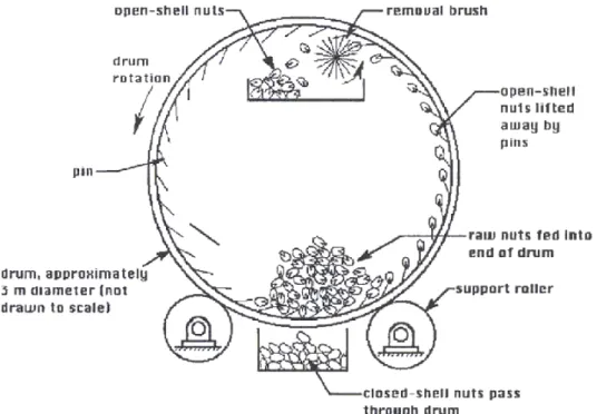
Figure 1.1: Schematic of a typical mechanical system for separating closed-shell from open-shell pistachio nuts. Courtesy of T. Pearson [1].

is critical to separate the pistachio nuts according to their openness. One of the mechanical systems is illustrated in Figure 1.1, which separates open pistachio nuts from the closed ones by picking the open pistachios up by a pin. However, this type of system has a large classification error and there are many open-shell pistachio nuts in closed-shell nuts.

The main quality measure for the hazelnut is the ratio of the kernel weight to shell weight. Underdeveloped hazelnuts and hazelnuts containing underdeveloped kernels negatively affect this ratio. If the ratio of kernel weight to gross weight is less than 0.5 then some buyers reject the produce. Sometimes, a physiological disorder such as plant stress from dehydration or lack of nutrients causes a hazel-nut shell to develop without a kernel. In addition, a physical disorder such as insect damage can stunt the maturation process and prevent a kernel from being fully developed at harvest time. A nut with underdeveloped kernel appears like

CHAPTER 1. INTRODUCTION 3

(a) (b)

Figure 1.2: The picture of underdeveloped (a) and full (b) hazelnuts. A nut with underdeveloped kernel appears like a normal hazelnut from outside.

a normal hazelnut from outside as seen in Figure 1.2. Currently, raw hazelnuts are processed by an “airleg” which is a pneumatic device to separate underde-veloped hazelnuts from fully deunderde-veloped ones. However, these devices have high classification error rates. There remains a need for more advanced systems to improve upon the segregation of underdeveloped and full hazelnuts. In addition, underdeveloped hazelnuts and hazelnuts containing underdeveloped kernels may also contain the mold, Asperguillus flavus, which produces aflatoxin, a cancer causing material [2]. Therefore, a more accurate classification of hazelnuts will enhance food safety.

The kernel damage is one of the biggest reasons that degrade the quality of flour. Such damage may occur in the form of fungal damage, and insect damage. The fungi type can infect kernels before and after harvest. The most important of these is Fusarium graminearum, which creates “scab” damage and may lead to toxins known to cause cancer [3]. On the other hand, internal insect infestation degrades the quality and value of wheat and is one of the most difficult defects to detect. The kernels become infested when an adult female insect chews a small hole into the kernel, about 0.05 mm in diameter, deposits an egg, and then seals

CHAPTER 1. INTRODUCTION 4

the egg with a mixture of mucus and the wheat that was chewed out. In the pupae stage, the egg plug is the same color as the wheat surface so it is nearly impossible to detect by external examination. When the egg hatches, the insect larvae develop and consume tunnels inside the wheat kernel until it reaches maturity. Finally, the insect exits the kernel by chewing an exit tunnel,“Insect Damaged Kernel” (IDK). Infestation causes grain loss by consumption, contaminates the grain with excrement and fragments, causes nutritional losses, and degrades end-use quality of flour [4]. Levels of insect infestation are a major factor in the grading of wheat quality. Therefore their percentage in the production/market is limited by Food and Drug Administration(FDA) and United States Department of Agriculture (USDA) standards [5].

Chapter 2

Kernel Processing and Aflatoxin

2.1

Produce Processing Techniques

2.1.1

Pistachio Processing

California pistachios are harvested in a period of two to three weeks in September. They can be harvested when hulls of pistachios are ready to be separated from the nut. Early harvest causes lots of underdeveloped pistachio nuts and late harvest causes more nuts with toxin materials. Pistachios are collected by shaking the tree and cause them to drop onto a collector. These nuts are carried to larger trailer bins to be processed in the pistachio plant. Nuts are carried to these larger bins in 24 hours after harvest. Pistachios and unwanted materials such as leaves are separated and pistachios are hulled. After these processes, pistachios are put into a water tank. The unhulled pistachios, most of the closed pistachios and hull material floats while open shell pistachios sinks. The nuts are dried after this process and put into a dry storage to be processed in the plant.

After the harvest is ended, these pistachios in storages are sorted according to their size and color. The hull material can cause pistachio nuts to change the color of their shells. These pistachios are not appropriate to be sold directly to

CHAPTER 2. KERNEL PROCESSING AND AFLATOXIN 6

the consumers. They can be used in processed produces (e.g., cake, ice cream). They are sorted by an electronic monochrome color sorter machine by comparing the nut with a background which has the same color as nut. There are more then one type of pistachio trees, but, Pistachio vera is the only one of these types that has sufficiently big fruits. Pistachio vera is also the only pistachio tree that has open shells. Pistachio trees do not produces the same amount of fruits every year. Actually they produce more fruits one year and less for next year. The pistachio tree in California is developed in 1929 from the Iranian and Turkish seeds by the US. Department of Agriculture. This US pistachio trees have large fruits and high capacity.

2.1.2

Hazelnut Processing

Hazelnut is widely consumed in all over the world. Turkey produces 75% of the world hazelnut production and Turkey is the largest hazelnut (85% worldwide) exporter too. Turkey exports 80% of its hazelnut production and 20% is consumed in national markets. The 80% of hazelnuts is used for chocolate industry, 15% of hazelnut is used for making cake, biscuit and candy, and 5% of hazelnut is consumed directly [6]. Hazelnut is a very nutritive produce and has a special taste. Hazelnut contains vitamin E, vitamin B6, calcium, potassium and iron. There are nearly 2 million people those are involving in the hazelnut industry in Turkey. Turkey gains approximately 1 billion US dollars per year from hazelnut exportation.

There are two types of hazelnuts. The first type is Giresun Type hazelnut, which is generally grown in Giresun region of Turkey. Giresun Type hazelnuts are well rounded and the highest quality hazelnut in the world. Other type of hazelnut is the Levant Type which is grown in the northern regions other than Giresun region. Levant Type hazelnuts have less fat than Giresun Type, however they are more delicious and they are hazelnuts of better quality than any other countries.

CHAPTER 2. KERNEL PROCESSING AND AFLATOXIN 7

on the place of orchard. There are two types of harvest method. First one is to drop the nuts down to the ground by shaking the tree. Second type is to directly collect the nuts from tree by hand. First method is better however it is not applicable for all hazelnut trees. The hazelnuts are spread onto the ground to change their hull color. After this process hazelnut fruit is separated from its hulls by a mechanical machine and again they spread onto the ground to dry again. The drying takes from 10 to 15 days. The dried hazelnuts are separated by another mechanical machine into underdeveloped and full hazelnuts. The hazelnut experts examine these separated hazelnuts and decide to buy or reject the hazelnut according to underdeveloped hazelnut to the full hazelnut ratio.

2.1.3

Wheat Processing

Wheat plant can be grown in many climates. Wheat requires a dry and hot weather; otherwise its color can not be change to golden. For instance, corn is used instead of wheat in northern Turkey . In Turkey, 20 million tones of wheat kernel are produced.

The harvest time of wheat is changing according the climate. The harvest starts in southern regions in early June, it continues in many regions in July and finally it ends in eastern Turkey which has a high altitude in August. Wheat is harvested by combine. It is very important to adjust the combine according to the operator’s manual, because wheat yield depends on this adjustment. If it is not adjusted, some of the wheat kernels can drop to the wheat field. After harvesting the wheat it should be removed from the field as soon as possible. Wheat is stored in a cool and dry bin to decrease the insect activity, to prevent growth of storage mold and moisture.

CHAPTER 2. KERNEL PROCESSING AND AFLATOXIN 8

2.2

Aflatoxin

Aflatoxin is a toxic compound produced by a mold fungus, Aspergillus flavus, in agricultural crops, especially peanuts, corn, rice, soybeans, pistachio nuts, hazelnuts, and in animal feeds that have not been carefully stored [7]. Aflatoxin can cause liver damage in humans, reduce the growth rate. Aflatoxin has caused deaths in farm animals that consumed heavily infected feed [8]. Aflatoxin caused hepatitis and death in more than 100 people who consumed severely infected corn [9]; but, it is unusual to find food infected with aflatoxin to the degree that it causes immediate health problems. Aflatoxin is also a known cancer-causing substance that has been traced to increased chances of liver cancer after repeated consumption of low levels (above 20 ppb.) of infected food [9]. Dichter et al. [10] estimated that due to aflatoxin exposure in the United States, 58 to 158 people per year are inflicted with liver cancer. However, Yeh [11] reported that, in southeast China where food regularly contains high aflatoxin concentrations, 91% of the liver cancer deaths in this area were in people who also tested positive for hepatitis B1. Thus, people likely to be inflicted with liver cancer due to aflatoxin may also have had hepatitis B1.

Agricultural kernels are sensitive to storage conditions. In a short time period they can be contaminated with aflatoxin if the storage conditions are suitable for aflatoxin contamination. This infection may cause quality decrease in agricultural kernels. For instance, in hazelnut kernels, the contamination causes the kernels to lost weight and results empty kernels. These nuts can also be classified as underdeveloped hazelnuts, since underdeveloped kernels are also empty. In this way, people can be protected from aflatoxin caused diseases by our proposed system.

Chapter 3

Methods, Materials and Results

The main problem for developing a classification algorithm is the feature extrac-tion. People generally do not sure which feature of a given signal is appropriate for the signal. We have developed several feature extraction methods by process-ing the impact sound signal of hazelnut kernels and wheat kernels to determine which features are more important for a particular kernel. We will introduce the previous work of T. Pearson et. al. [12] and then present our work [13] about hazelnut kernels and wheat kernels.

3.1

Previous Work

In this work, Pearson et. al. [12] construct a prototype to classify the impact sound of California pistachio nuts. The prototype of the system, methods and results are presented in the following sections.

3.1.1

Pistachio Setup

The system was designed to feed pistachio nuts to an impact plate, record the sound from the impact of pistachio on this impact surface, process the data

CHAPTER 3. METHODS, MATERIALS AND RESULTS 10

according to the proposed feature extraction algorithms and classify the pista-chios into either a closed shell or open shell pistachio as illustrated in Figure 3.1. Actually, the real-time system with a DSP processor is constructed at Bilkent University as seen in Figure 3.2.

Figure 3.1: Schematic of pistachio sorter based on acoustic emissions. Courtesy of T. Pearson [1].

The slide was constructed of polished stainless steel angle iron to form a declining to an impact plate. Impact plate is made of 50.8 × 50.8 mm polished stainless steel bar. The mass of the plate should be large enough to eliminate vibrations when the pistachio nut impacts.

A highly directional “shotgun” microphone was used to minimize the sur-rounding sound effects. Output of microphone is connected to electronic card that can perform several arithmetic operations in real time. This card has a sampling frequency of 192kHz. When the pistachio nut drops onto the plate, the photo detector sends a signal to the electronic card to start the recording. If the dropped pistachio nut is classified as an open shell nut then an air valve is used to

CHAPTER 3. METHODS, MATERIALS AND RESULTS 11

Figure 3.2: Picture of pistachio sorter based on acoustic emissions at Bilkent University.

reject this open shell pistachio nut. In this way open and closed shell pistachios are detected and separated.

3.1.2

Melcepstrum

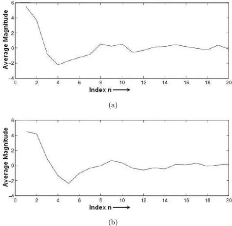
The duration of the impact sound from pistachio nuts is much shorter than a typ-ical word and some phonemes; therefore, only one short-time window of duration 1.4 ms was used and only one set of mel-cepstrum coefficients was computed for each nut. Let x be a vector containing N sound samples; mel-cepstrum coeffi-cients are obtained by the following computations:

• Discrete Fourier transform (DFT) of the data vector x is computed using

CHAPTER 3. METHODS, MATERIALS AND RESULTS 12

• The DFT (ˆx) is divided into M non-uniform sub-bands, and the energy (i.e., i = 1, 2, . . . , M) of each sub-band is estimated. The energy of each sub-band is defined as ei =

q

P

l=p

| ˆx (l) |2, where p and q are the indices of sub-band edges in the DFT domain. The sub-bands are distributed across the frequency domain according to a “mel-scale” which is linear at low fre-quencies and logarithmic thereafter. This mimics the frequency resolution of the human ear. Below 10 kHz, the DFT is divided linearly into 12 bands. At higher frequency bands, covering 10 to 44 kHz, the sub-bands are divided in a logarithmic manner into 12 sections. In this case, the Fourier domain is divided linearly into 12 bands below 10 kHz, and the frequency range cover-ing higher frequencies from 10 to 44 kHz is divided in a logarithmic manner into 12 sections. Therefore, more emphasis is given to low-frequency infor-mation than to high-frequency data. In other words, the DFT coefficients are grouped into M = 24 sub-bands in a non-uniform manner.

• The mel-cepstrum vector c = [c1, c2, . . . , cK] is computed from the discrete

cosine transform (DCT) [14]: ck = M X i=1 log (ei) cos [k (i − 0.5) π/M] , k = 1, 2, ..., K (3.1)

where the size of the mel-cepstrum vector (K) is much smaller than data size N. The mel-cepstrum sequence is a decaying sequence for sound signals. A value of 20 was chosen for K, as coefficients with an index greater than K = 20 are usually negligible. The DCT has the effect of compressing the log-spectrum, thereby providing a small set of coefficients representing most of the variance of the original data set. Another advantage of the DCT is that it is close to the optimum Karhunen-Loeve transform [15] of highly correlated random processes; thus, it approximately de-correlates the mel-scale logarithmic sub-band energies. The basis of the DCT resembles the basis of the Karhunen-Loeve transform, which is obtained by eigen-analysis of the autocorrelation matrix of the data. De-correlated coefficients are more suitable to modeling than De-correlated coefficients. In automatic speech and speaker recognition, it is observed that mel-cepstrum

CHAPTER 3. METHODS, MATERIALS AND RESULTS 13

coefficients (ck) give better recognition performance than sub-band energies (ei)

or logarithmic sub-band energies, log(ei) [16].

(a)

(b)

Figure 3.3: Mel-cepstral coefficients of a pistachio nut with (a) open shell and (b) closed shell.

3.1.3

Principle Component Analysis (PCA)

Let C be the correlation or covariance matrix:

C = E[(x − xm)(x − xm)T] (3.2)

where x represents the random sound vector, and xm is the mean of x. The

matrix C is an N by N matrix, where N is the size of data vector x. The eigenvectors of this matrix represent the projection axes, or eigen-sounds of the

CHAPTER 3. METHODS, MATERIALS AND RESULTS 14

data, and the eigenvalues represent the projection variance of the corresponding eigen-sound. The eigenvectors correspond to large eigenvalues of C are usually chosen as projection axes, as these explain most of the variance of the original data set before the transformation. The correlation matrix is estimated from the training set of L sound vectors (x1, x2, ..., xL) as follows:

Let X = [(x1− xm)(x2− xm) ... (xL− xm)] be the matrix of the training

vectors obtained by concatenating the sound vectors. The mean vector (xm) is

the average vector of the data set. An estimate of C is given by Ce = XXT. The

rank of matrix Ce is less than or equal to L. Usually, the training vectors are

linearly independent of each other; therefore, Ce has L non-zero eigenvalues:

XXTuk = λkuk , k = 1, 2, . . . , L (3.3)

where λk and uk are the eigenvalues and eigenvectors of Ce, respectively. The

largest L0 _{out of L eigenvalues are usually selected as a representative set of data,}

and the corresponding eigenvectors are used in the PCA analysis-based recog-nition systems. Projections of a sound vector (x) onto the first L1 eigenvectors

define a feature vector representing the signal x:

ω_x = [ωx,1ωx,2... ωx,L1] (3.4)

where ωx,k = uk· (x − xm)

In some practical situations, Ce is too large for eigenvalue and eigenvector

estimation. This was the case with the pistachio data set used in this study, as x contains N = 350 sound samples. This difficulty can be overcome by noting that the eigensystem of XT_{X has the same non-zero eigenvalues as C}

e, since

XXTXuk= λkXuk, where λkand ukare the eigenvalues and eigenvectors of Ce,

respectively. As a result, the reduced eigensystem of XT_{X ∈ R}LxL _{can be solved}

instead of Ce, as the size of the training set (L) is usually less than the number

of samples (N) in each data vector (x). The new eigenvalues are the same as eigenvalues of the original system, but eigenvectors are wk= Xuk.

CHAPTER 3. METHODS, MATERIALS AND RESULTS 15

3.1.4

Minimum Distance classifier

Minimum distance classifier uses a training set to estimate means, which are used to compute Euclidean distances from an unknown sample to the centroid of each class. The unknown sample is then classified into the class associated with the smallest Euclidean distance to the group centroid. The line where the Euclidean distance from each class is equal forms the decision boundary between the classes. This method assumes spherical Gaussian distributions of the data, and works well when the data is fairly well clustered.

3.1.5

Pistachio Nut Results

Pistachio nuts are classified using Principle Component Analysis (PCA) of Mel-cepstrum coefficients and PCA of the sound amplitudes. The feature vectors are fed into a minimum distance classifier. We also examine the effects of training set size on the results.

In Table 3.1, classification results based on PCA of sound amplitudes are presented. The first column lists the number of training sounds for each class. The second and third columns list the percentage of correctly classified closed-and open-shell nuts in the validation set containing 280 sounds, except for the bottom row in which the validation set size was 270 because 30 nuts were used for training.

Only two out of 280 closed-shell nuts were misclassified in all cases, corre-sponding to 99.3% recognition accuracy for closed-shell nuts. The number of misclassified open-shell nuts decreased as the number of training sounds increased, up to the case in which 20 sound vectors were used in training each representative vector. Beyond this level, improvement in the recognition performance was not observed.

In Table 3.2, classification results based on PCA of the mel-cepstrum coeffi-cients are presented. The first column lists the number of nuts used for training

CHAPTER 3. METHODS, MATERIALS AND RESULTS 16

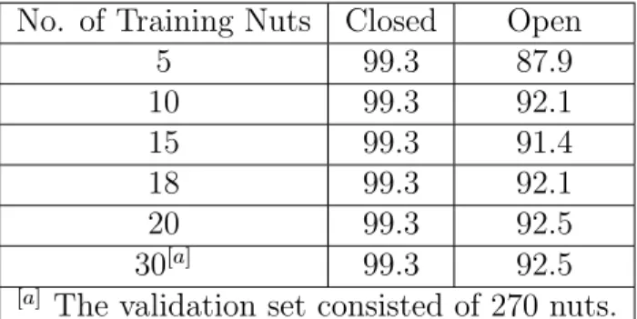
Table 3.1: Classification results for PCA of mel-cepstrum coefficients. The second and third columns present the percent of correctly classified closed- and open-shell nuts in a validation set containing 280 sounds.

No. of Training Nuts Closed Open

5 99.3 87.9 10 99.3 92.1 15 99.3 91.4 18 99.3 92.1 20 99.3 92.5 30[a] _{99.3 92.5} [a] _{The validation set consisted of 270 nuts.}

for each class. The second and third columns list the percentage of correctly classified closed- and open-shell nuts in the validation set containing 280 sounds. Open-shell nuts were correctly classified in all cases.

Table 3.2: Classification results for PCA of mel-cepstrum coefficients. The second and third columns present the percent of correctly classified closed- and open-shell nuts in a validation set containing 280 sounds.

No. of Training Nuts Closed Open

5 76.7 100

10 82.9 100

15 91.8 100

20 93.2 100

The method based on PCA features of sound amplitudes classified closed-shell nuts more accurately than open-closed-shell nuts. On the other hand, the method based on mel-cepstral features classified open-shell nuts more accurately than closed-shell nuts, as shown in Table 3.2. The most accurate recognition results were obtained when PCA of sound amplitudes was combined with mel-cepstral features, as summarized in Table 3.3.

The number of misclassified open-shell nuts dropped to four, which corre-sponds to 98.6% recognition accuracy in open-shell nuts when the training set comprised 20 closed-shell nuts and 20 open-shell nuts (bottom row of Table 3.3).

CHAPTER 3. METHODS, MATERIALS AND RESULTS 17

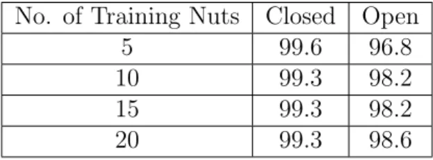
Table 3.3: Classification results for both PCA of sound amplitudes and mel-cepstrum coefficients. The second and third columns present the percent of cor-rectly classified closed- and open-shell nuts in a validation set containing 280 sounds.

No. of Training Nuts Closed Open

5 99.6 96.8

10 99.3 98.2 15 99.3 98.2 20 99.3 98.6

Recognition accuracy of the closed-shell nuts remained the same (99.3%) after linear combination.

3.2

Hazelnut Work

3.2.1

Setup

The hazelnut setup is similar to pistachio nut setup. They have impact plates which are fed by chute or slide. Some of the setup components such as micro-phones and impact plates are different.

In order to inspect nuts at high throughput rates, a prototype system was set up to drop nuts onto a steel plate and process the acoustic signal generated when nuts hit the plate. It is possible to process and reject 20-40 nuts per second by the proposed system. Underdeveloped nuts could be removed by activation of an air valve; however, this was not included for the hazelnut case as the main objective was to ascertain the feasibility of detecting underdeveloped hazelnuts by this method.

An experimental apparatus was fabricated to slide hazelnuts down a chute and project them onto an impact plate, then collecting the acoustic emissions from the impact. The impact plate was a polished block of stainless steel with dimensions

CHAPTER 3. METHODS, MATERIALS AND RESULTS 18

(a) (b)

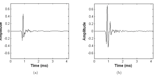
Figure 3.4: Typical impact sound signals from an (a) underdeveloped hazelnut and (b) a full hazelnut. Note that the extremum of a full hazelnut is usually higher than an underdeveloped hazelnut.

75 × 150 mm and depth of 20 mm. The mass of the impact plate is much larger than the hazelnuts in order to minimize vibrations from the plate interfering with acoustic emissions from hazelnuts. A microphone, which is sensitive to frequencies up to 20 kHz, was used to capture impact sounds. The sound card in a typical personal computer was used to digitize and store the microphone signals for analysis. The sampling frequency of the impact sound was 48 kHz. A sample sound signal from underdeveloped and full hazelnuts is illustrated in Figure 3.4 and sample sounds from 200 full and 200 underdeveloped hazelnuts are illustrated in Figure 3.5.

3.2.2

Weibull Curve Fitting and Weibull Function

Param-eters

The shape of the time domain signal of underdeveloped and full hazelnuts is different. The typical signals from underdeveloped and full hazelnuts can be seen

CHAPTER 3. METHODS, MATERIALS AND RESULTS 19

(a)

Figure 3.5: Underdeveloped (top 200 rows) and full (bottom 200 rows) hazelnut records. Each row represents a record.

in Figure 3.4. This feature extraction method is also used to separate the healthy wheat kernels from the insect damaged wheat kernels.

The extremum of the signals is quite variable but, in general, the extremum of full hazelnuts is higher than the underdeveloped ones. This is also valid for wheat kernel sounds. To characterize this type of signal response, the signal was modeled after transforming it in the following steps outlined below:

i. Rectify the signal by taking the absolute value at all points

ii. Non-linearly filter the signal by replacing the center data point with the maximum value in a seven point window

CHAPTER 3. METHODS, MATERIALS AND RESULTS 20

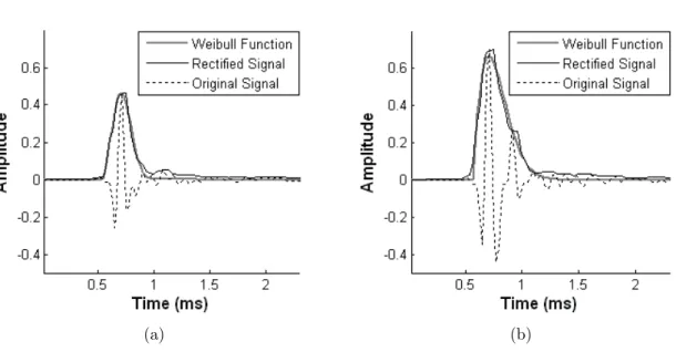
(a) (b)

Figure 3.6: Typical (a) underdeveloped and (b) full hazelnut impact sounds with the rectified signals and Weibull functions which are fit to rectified signals.

iii. Estimate the four parameters of the Weibull function given by Equation 3.5, which has a shape similar to the envelope of the processed time domain signal.

Y (t) = ( cb a £_t−t 0 a ¤_b−1 e−[t−t0a ] b , for t > t0 0 ,otherwise (3.5)

Figures 3.6 and 3.7 show how Weibull function curve fits to the rectified hazelnut and wheat impact sounds.

3.2.3

Exponential Function Fitting and Exponential

Function Parameters

The Weibull curve fitting is quite complex for a real-time application. A similar but more simple functions can be used to model the impact sound in time do-main. One of those functions is the exponential function with two parameters. We used the same procedures as explained in Section 3.2.2 to characterize the

CHAPTER 3. METHODS, MATERIALS AND RESULTS 21

(a) (b)

Figure 3.7: Typical (a) insect damaged kernel (IDK) and (b) good wheat impact sounds with the rectified signals and Weibull functions which are fit to rectified signals.

type of signal response. The only difference is we fit an exponential function as shown in Equation 3.6 to the rectified signal instead of Weibull function. The computation of exponential curve fitting takes less time than the computation of Weibull function.

Y (t) = ae−_bt _(3.6)

Figures 3.8 and 3.9 show how Exponential function curve fits to the rectified hazelnut and wheat impact sounds.

CHAPTER 3. METHODS, MATERIALS AND RESULTS 22

(a) (b)

Figure 3.8: Typical (a) underdeveloped and (b) full hazelnut impact sounds with the rectified signals and Exponential functions which are fit to rectified signals.

(a) (b)

Figure 3.9: Typical (a) Insect Damaged Kernel (IDK) and (b) Good wheat kernel impact sounds with the rectified signals and Exponential functions which are fit to rectified signals.

CHAPTER 3. METHODS, MATERIALS AND RESULTS 23

3.2.4

Short Time Variances in Windows of Data

In addition to Weibull function, based envelope modeling of impact sounds, vari-ances of these signals are also computed in short time windows. Weibull function captures the shape of the recorded signal globally and the short-time variance information models the local time domain variations in the signal. The short time windows were 50 points in duration and incremented in steps of 30 points so that each window overlapped by 20 points. The first window began 40 points in front of the extremum. Eight short time windows were computed to cover the entire duration of all impact signals. After all variances were computed, they were normalized by the sum of all eight variances as follows

σni2 = σi 2 8 P i=1 σi2 (3.7) (a) (b)

Figure 3.10: (a) Variances of short time windows of time domain signals in Fig-ure 3.4 and (b) average variances from short time windows of time domain signals. The parameters σni2 and σi2 are the normalized and computed variances from

CHAPTER 3. METHODS, MATERIALS AND RESULTS 24

captures the increased duration of the signals from underdeveloped hazelnuts. As it is seen from Figure 3.10, the average normalized variances of the last three windows are greater than that from full hazelnuts.

3.2.5

Line Spectral Frequencies (LSFs)

Linear predictive modeling techniques are widely used in various speech coding, synthesis and recognition applications [16]. Linear Minimum Mean Square Error (LMMSE) prediction based data analysis is equivalent to Auto-Regressive (AR) modeling of the data. Line Spectral Frequency (LSF) representation of the Linear Prediction (LP) filter was introduced by [17] and used in common cell phone communication systems including the GSM and MELP speech coding systems, [16]. In LMMSE analysis, it is assumed that the sound data can be modeled using an m − th order linear predictor, i.e. xp[n] = a1x [n − 1] + a2x [n − 2] +

...amx [n − m] where x [n − k] is the sound sample at time instant (n − k) Ts is

the estimated sound sample at time instant nTs (Ts is the sampling period). The

error signal at index n is e [n] = x [n] − xp[n]. The filter coefficients ak are

determined by minimizing the mean-square error σ2

e = E

£

(x [n] − xp[n])2

¤ [18]. The following set of linear equations is obtained by taking the partial derivative of E£(x [n] − xp[n])2

¤

with respect to the filter coefficients and setting the results to zero r [0] a1 + r [1] a2 + r [2] a3 + ... + r [m − 1] am = r [1] r [1] a1 + r [0] a2 + r [1] a3 + ... + r [m − 2] am = r [2] r [2] a1 + r [1] a2 + r [0] a3 + ... + r [m − 3] am = r [3] : : : : + : : r [m − 1] a1 + r [m − 2] a2 + r [m − 3] a3 + ... + r [0] am = r [m]

where r [k] represents the autocorrelation sequence of the zero mean sound data

r [k] = E [x [n] x [n − k]]. In practice, the autocorrelation sequence is directly

estimated from the data, i.e. ˆr [k] = 1

N

N −1−|k|_P n=0

x∗_{[n] x [n + k] where N is the}

number of sound samples. In some cases, the above sum is normalized by (N − k) instead of N leading to an unbiased estimate of the autocorrelation sequence. Line spectral coefficients are computed from the linear prediction filter coefficients.The

CHAPTER 3. METHODS, MATERIALS AND RESULTS 25

so-called m−th order inverse polynomial Am(z) is defined as Am(z) = 1+a1z−1+

...+amz−m. The polynomial Am(z) is used not only in LSF computation but also

in spectrum estimation. Notice that σe2

Am(ejω) is called the autoregressive spectrum

estimate of the sound data. In speech processing m = 10 is selected for speech coding and recognition applications at a sampling frequency, fs, of 8000 Hz.

(a) (b)

Figure 3.11: Example frequency spectra magnitudes for an underdeveloped (a) and a full hazelnut (b). Vertical lines correspond to phase angles of LSFs for each nut.

In this thesis, LSFs are also used as feature parameters to represent im-pact sounds. The LSF polynomials of order m + 1, Pm+1(z) and Qm+1(z)

are constructed by setting the (m + 1)-st reflection coefficient to 1 or −1. In other words, the polynomials, Pm+1(z) and Qm+1(z) are defined as Pm+1(z) =

Am(z) + z−(m+1)Am(z−1) and Qm+1(z) = Am(z) − z−(m+1)Am(z−1). Zeros of

Pm+1(z) and Qm+1(z) are called the Line Spectral Frequencies (LSFs), and they

all lie on the unit circle in the complex z-domain. Zeros of Pm+1(z) and Qm+1(z)

uniquely characterize the LPC inverse filter Am(z), i.e., one can uniquely

con-struct the LP filter coefficients from the LSFs. Phase angles of the LSFs tend to concentrate around spectrum peaks as shown in Figure 3.11. In these plots phase angle range [0,π ] is mapped to range [0,24kHz] because the sampling frequency was 48kHz. Due to this interesting property, LSFs represent the spectrum of the

CHAPTER 3. METHODS, MATERIALS AND RESULTS 26

impact sound, and that is why they are selected as a set of sound features in this study.

The LSF order m = 10 was chosen because best classification accuracy was obtained when m = 10 as summarized in Tables 3.4 and 3.5. LSFs can be computed very efficiently in real-time [17].

3.2.6

Extrema in Short Time Windows

The first 165 samples from 30th _{sample of the impact sound was divided into 11}

no overlapping time domain windows and the extremum value of each window was selected as a feature value. Extrema in short-time windows also captures the envelope of the impact sound similar to the variances in short-time windows.

3.2.7

Frequency Domain Processing

A 256-point Discrete Fourier Transform (DFT) was computed from each signal using a Hamming window. The 256-point window covers the impact sound of hazelnuts starting at about 80 data points before the signal maximum slope, which corresponds to the impact moment of the kernel. The magnitude of each spectrum was computed and then low pass filtered using a 20-tap FIR filter applied to remove jagged spikes in the spectra. The low pass filter has a cutoff frequency of π

4 in the normalized DFT domain. As it is seen in Figure 3.11,

the frequency spectrum of underdeveloped nuts has a single major peak between 4 and 10 kHz. On the other hand, full hazelnuts generally have two peaks in the same frequency range. In this example, peaks of the spectra of full hazelnuts and underdeveloped nuts are clearly distinguishable; however there are significant numbers of examples in which twin peaks of full hazelnuts are not clearly visible, possibly due to noise. The frequency corresponding to the peak magnitude in the frequency spectra was saved as a potential discriminating feature. In addition, the 15 magnitude values before the peak and 15 points after the peak were saved and normalized by the peak magnitude.

CHAPTER 3. METHODS, MATERIALS AND RESULTS 27

3.2.8

Support Vector Machines

In a two-class problem, data on opposite sides of the centroids is given just as much importance as data in-between centroids of the two classes. Sometimes this data contributes to higher variance within a class and leads to erroneous classifications when minimum distance classifier is used. In contrast, support vector machines (SVM) Hearst [19], Sch¨olkopf et al. [20] and Burges [21] seek to define a boundary between classes that maximize the distance between training set samples from different classes that happen to lie near each other. For example, Figure 3.12 shows two hypothetical training sets that might be taken from a two class training set. SVM seeks to define a boundary between two classes as a line that intersects the minimum distance between the hulls (dotted line) between two groups. Thus, classification by SVM is concerned only with data from each class near the decision boundary, called support vectors, all other data is not relevant. Algorithms have been developed to compute the boundary line as a polynomial, sigmoid or radial basis function.

Support Vector Machine are used for isolated handwritten digit detec-tion [22, 23, 24, 25], object recognidetec-tion [26], face detecdetec-tion in images [27] etc. and were used in this study to detect underdeveloped hazelnuts from fully developed hazelnuts and healthy wheat kernels from insect damaged wheat kernels. SVMs classifier increases the dimension of feature space by using a mapping function, and linearly classifies the data in this dimensionally increased space. This effect causes SVMs classifier to be nonlinear in feature space. The mapping function maps a vector from a lower dimension to a higher or infinite dimension; how-ever, a kernel function is used instead of the mapping function for training the algorithm to ease computational load. Kernel functions are like vector multipli-cation operations, but the effect of the kernel function is to multiply the vectors in higher dimensions. Since the linear SVM algorithm only depends on the vec-tor multiplication, there is no need to know the mapping function, if the kernel function is given. In underdeveloped hazelnut detection, we used the radial base function (RBF). In addition, other base functions did not improve the classifica-tion accuracy for some examined cases. The SVM classificaclassifica-tion was performed

CHAPTER 3. METHODS, MATERIALS AND RESULTS 28

Figure 3.12: Decision boundary determination by SVM using a linear kernel: filled circles indicate feature vectors of the first class and underdeveloped circles indicate feature vectors of the second class, respectively. Line (or hyperplane in higher dimensions) separates the decision regions of the first and second classes.

using a software package called LIBSVM [28], which is a free SVM package. This package scales the features between minus one and one. In addition, a two fold cross validation is performed for non-randomly and randomly grouped data which makes four different results for each experiment. The final results are the average of these four experimental results. The LIBSVM package is written for many programming languages. We used the C version of the package for this study.

3.2.9

Hazelnut Results

The classification results using each type of feature are given Tables 3.4 and 3.5. The results using a combination of different feature types are given in Table 3.6.

CHAPTER 3. METHODS, MATERIALS AND RESULTS 29

1. Weibull parameters: In this case Weibull parameters a, b, c, and t0and R2(the

coefficient of multiple determination for curve fitting) were used as features of the hazelnut impact sound and a recognition accuracy of 95.2% is achieved in Levant type hazelnuts.

2. Exponential function parameters: The parameters a and b were used as a discriminating features of the hazelnut impact sound for this case. The recog-nition accuracy of 96.2% is achieved. This function has more accurate results than the Weibull parameters, moreover it is more simple and can be computed faster.

3. Eight short-time variances: Comparing these features with the other features, short-time window variances had the lowest classification performance, 89.8% in Levant type hazelnuts.

4. Maxima in time domain: These features had the highest classification accu-racy, 95.9% in Levant type hazelnuts.

5. Spectrum magnitude features: This feature vector alone leads to 93.8% recog-nition accuracy. Spectrum magnitude features classified underdeveloped hazel-nuts more accurately than full hazelhazel-nuts in Levant type hazelhazel-nuts.

6. 10th _{order Line Spectral Frequencies (LSFs): Overall recognition rate of 93.2%}

was achieved when m=10th _{order LSFs were used in Levant-type hazelnuts.}

Table 3.5 summarizes classification results for various order LSFs.

Table 3.4: Classification accuracies (%) obtained by different feature vectors for Levant type hazelnuts.

Features Underdeveloped Full Overall

Weibull 95.9 94.7 95.2 Exponential 96.4 96.0 96.2 Short-Time Variances 87.5 91.8 89.8 Short-Time Maxima 95.5 96.2 95.9 Spectrum Magnitudes 94.6 93.1 93.8 m = 10th _{order LSFs 93.8 92.7 93.2}

CHAPTER 3. METHODS, MATERIALS AND RESULTS 30

Table 3.5: Classification accuracies (%) obtained by various orders of LSFs for Levant type hazelnuts.

Order (m) Underdeveloped Full Overall

8 94.0 88.9 91.3

9 95.7 88.7 92.0

10 93.8 92.7 93.2

11 94.0 89.1 91.4

12 92.2 91.8 92.0

Table 3.6: Classification results obtained by composite feature vector contain-ing Weibull parameters and short-time variances for Levant and Giresun Type Hazelnuts.

Levant Type

Underdeveloped Full Overall Weibull and Extrema 96.1 97.7 97.0 Exponential and Extrema 96.1 97.7 97.0

All Features 96.8 96.8 96.8

Extrema and LSFs 96.8 96 96.4 Giresun Type

Underdeveloped Full Overall Variances, Extrema and LSFs 90.6 96.8 94.4 Weibull and LSFs 87.5 98.1 94.0 Extrema and LSFs 86.5 98.1 93.7

When all feature parameters were combined into a single vector and an SVM with radial basis function kernel was used, an overall recognition accuracy of 96.8% was achieved, as shown in Table 3.6. Similar results were obtained with SVMs using sigmoid and polynomial kernel functions. When Weibull parame-ters and maxima parameparame-ters were combined into a feature vector, a recognition accuracy of 97% was achieved. The feature vector comprising LSFs and time-domain maxima information produced 96.8% classification accuracy for Levant-type hazelnut. In Giresun Type hazelnuts, recognition rates were slightly lower; this might be due to the smaller size of the data set. It may not be possible to capture all the information about a classification problem with a small training set. In this case, LSFs, short time variance, and maxima information produced

CHAPTER 3. METHODS, MATERIALS AND RESULTS 31

94.4% classification accuracy. In addition, feature vectors comprising Weibull parameters and LSFs had a classification accuracy of 94% for Giresun Type nuts. Computation of Weibull parameters is an iterative process and can occasionally take over 20ms to perform. More computationally efficient algorithms exist for the other feature parameters, which can all be computed in real-time to realize a system capable of processing more than 40 nuts/sec. Therefore, a feature vec-tor combining LSFs and time-domain maxima appears best for classification of underdeveloped and full hazelnuts in real-time applications. This vector carries both time and frequency information of impact sounds.

3.3

Wheat Work

3.3.1

Wheat Setup

A schematic of the experimental apparatus for dropping wheat kernels onto the impact plate, then collecting the acoustic emissions from the impact is shown in Figure 3.1 which is same as the pistachio setup. The impact plate was a polished block of stainless steel approximately 7.5 × 5.0 × 10 cm. The mass of the impact plate is much larger than the wheat kernels in order to minimize vibrations from the plate interfering with acoustic emissions from kernels. A microphone, which is sensitive to frequencies up to 100 kHz, is used in order to sense ultrasonic acoustic emissions from the wheat kernels. Microphone signal is digitized at a sampling frequency of 192 kHz with 16 bit resolution. The data acquisition was triggered using an optical sensor. After acquisition, the signal was first high pass filtered using a single pole recursive filter with a cutoff frequency of 9,600 kHz to eliminate 60 Hz noise, any DC offset.

3.3.2

Wheat Kernel Results

There are two types of kernels in our experiments. The first one is the healthy kernels without insect infestation (GOOD) and the second type of wheat kernel

CHAPTER 3. METHODS, MATERIALS AND RESULTS 32

is the insect damaged kernels (IDK).

The Weibull curve fit parameters a, b, c, t0 and R2, all eight normalized

variances from the short time windows, the frequency corresponding to the peak DFT magnitude, 15 normalized DFT magnitudes before and after the peak DFT magnitude, 20th _{order LSFs, and 11 extrema values were combined and used}

as potential discriminating features. Besides, each type of features are used to classify good and IDK kernels. The results are tabulated in Table 3.7

Table 3.7: Classification accuracies (%) obtained by different feature vectors for wheat kernels.

Features IDK GOOD Overall Weibull 86.3 94.0 91.0 Short-Time Variances 86.1 94.0 91.0 Short-Time Maxima 81.9 90.8 87.3 Spectrum Magnitudes 83.1 96.0 91.0 10th _{order LSFs 73.8 92.8 85.4} All Features 84.4 97.2 92.2

Chapter 4

Conclusion

A method, based on voice-recognition technology, was developed for detecting several types of agricultural produces that may emit sound when they his a steel plate. We deal with three types of agricultural produces, namely pistachio nuts, hazelnuts and wheat kernels.

The methods in this thesis appear to be as accurate as the method developed by Pearson [1]. Most importantly, they are low-cost sound based methods and they can be implemented in real-time.

T. C. Pearson et. al. [12] used impact sounds of pistachio nuts in mel-cepstral coefficients and PCA based classification system. The computational cost of training phase of this system is higher than the recognition phase. In practice training can be done off-line. Because the eigenvalues and eigenvectors of a large dimension matrix are computed. On the other hand, the testing phase is simply a matrix and a vector multiplication, so it can be implemented in real-time. Furthermore a simple linear algebraic trick, as explained in Section 3.1.3, can be used to cope with this computation difficulty.

Impact sounds of hazelnuts were analyzed and feature parameters describing time and frequency domain characteristics of the acoustic emission signals were extracted and combined into a feature vector. The feature vector obtained by

CHAPTER 4. CONCLUSION 34

combining LSFs and time-domain maxima, having both time and frequency in-formation of the impact sound, enabled classification of underdeveloped and full hazelnuts with over 97% accuracy by using an SVM-based classifier for Levant-type hazelnuts. The protoLevant-type classification system uses computationally efficient features and methods, thus requiring only modest computing hardware. The pro-posed system has the capacity to process 20-40 nuts per second in real-time.

Hazelnut methods are also used to extract features from the wheat kernel impact sounds. The recognition accuracy with over 92% is obtained with an SVM classifier. These sounds have interesting waveforms. Some of the recordings have virtually no signal or the amplitude of impact sound signal is too small compared to the other records. However, we did not exclude these sounds and this situation may affect the recognition accuracy for wheat kernels.

As a result, a low-cost, real-time sorting algorithms are proposed in this thesis for some agricultural kernels. We introduced methods used by T. Pearson et. al. [12] for pistachio nuts and proposed new methods for hazelnuts and wheat kernels. Our proposed methods have similar classification accuracies as the pistachio nut methods. These methods can be used to pick up the poor quality produce from a mixture of good and poor quality produces for increasing the average produce quality. In this way people will be healthier and lots of good quality produce will be saved from getting into garbage.

Bibliography

[1] T. C. Pearson, “Detection of pistachio nuts with closed shells using impact acoustics,” Applied Eng. in Agric, vol. 17, no. 2, pp. 249–253, 2001.

[2] I. M. Marklinder, M. Lindblad, A. Gidlund, and M. Olsen, “Consumers’ ability to discriminate aflatoxin-contaminated brazil nuts,” Food Additives

and Contaminants, vol. 22, pp. 56–64, January 2005.

[3] C. M. Christensen and R. A. Meronuck, Quality Maintenance in Stored

Grains and Seeds. Minneapolis, MN: University of Minnesota Press, 1986.

[4] USDA. Electronic code of federal regulations Title 7 (Agriculture) Chapter VIII (Federal Grain Inspection Service) Part 810 (Official United States Standards for Grain).

[5] J. Pederson, Insects: Identification, damage, and detection. In Storage of

Cereal Grains. Saint Paul, MN: American Association of Cereal Chemists,

1992. ed. D. B. Sauer.

[6] N. Altunda˘g, “Gıdalar K¨ufler ve Mikotoksinler Projesinde T ¨ UB˙ITAK-F˙ISKOB˙IRL˙IK ˙I¸sbirli˘gi C¸ er¸cevesinde F˙ISKOB˙IRL˙IK’te Yapılan C¸ alı¸smalar,” in Gıdalar K¨ufler ve Mikotoksinler Sempozyumu Tebli˘gleri, (˙Istanbul), 1989.

[7] A. Ciegler, “Mycotoxins: Occurrence, chemistry, biological activity.,”

Lloy-dia, vol. 39, no. 21, 1975.

BIBLIOGRAPHY 36

[8] A. Farsaie, W. McClure, and R. Monroe, “Design and development of an au-tomatic electro-optical sorter for removing BGY fluorescent pistachio nuts,”

Transactions of the ASAE, vol. 24, no. 05, pp. 1372–1375, 1981.

[9] U. Samarajeewa, A. C. Sen, M. Cohen, and C. Wei, “Detoxification of afla-toxins in foods and feeds by physical and chemical methods,” Journal of

Food Protection, vol. 53, no. 6, pp. 489–501, 1990.

[10] C. R. Dichter, “Risk estimates of liver cancer due to aflatoxin exposure from peanuts and peanut produces,” Food Chemistry and Toxicology, vol. 22, no. 6, pp. 431–437, 1984.

[11] F. S. Yeh, M. C. Yu, C. C. Mo, S. Luo, M. J. Tong, and B. E. Hender-son, “Hepatitis B virus, aflatoxins, and hepatocellular carcinoma in southern guanxi, china,” Cancer Research, vol. 49, pp. 2506–2509, 1989.

[12] A. E. C¸ etin, T. C. Pearson, and A. H. Tewfik, “Classification of closed and open-shell pistachio nuts using voice-recognition technology,” Trans. Of Am.

Soc. Of Ag. Eng., vol. 47, pp. 659–664, March/April 2004.

[13] A. E. C¸ etin, ˙I. Onaran, T. C. Pearson, Y. Yardımcı, and B. D¨ulek, “Detec-tion of empty hazelnuts from fully developed nuts by impact acoustics,” in

European Signal Processing Conference, (Antalya), September 2005.

[14] N. Ahmed, T. Natarajan, and K. R. Rao, “Discrete Cosine Transform,”

IEEE Trans. Computer, vol. C-23, pp. 90–93, Jan 1974.

[15] N. S. Jayant and P. Noll, Digital Coding of Waveforms. Englewood Cliffs, N. J.: Prentice-Hall, 1984.

[16] T. Quatieri, Discrete-Time Speech Signal Processing: Principles and

Prac-tice. Prentice-Hall, 2001.

[17] F. Itakura, “Line spectrum representation of linear predictive coefficients of speech signal,” J. Acoust. Soc. Amer., vol. 57, p. 535, April 1975.

[18] S. K. Mitra, Digital Signal Processing. McGraw-Hill Education, Second ed., 2002.

BIBLIOGRAPHY 37

[19] M. A. Hearst, “Support Vector Machines,” IEEE Intelligent Systems, vol. 13, no. 4, pp. 18–28, 1998.

[20] B. Sch¨olkopf, C. J. C. Burges, and A. J. Smola, Introduction to Support

Vector Learning, in Advances in Kernel Methods: Support Vector Learning.

Cambridge, MA: MIT Press, 1999.

[21] C. J. C. Burges, “A Tutorial on Support Vector Machines for Pattern Recog-nition,” Data Mining and Knowledge Discovery, vol. 2, no. 2, pp. 121–167, 1998.

[22] C. Cortes and V. Vapnik, “Support vector networks,” Machine Learning, vol. 20, pp. 273–297, 1995.

[23] B. Sch¨olkopf, C. Burges, and V. Vapnik, “Extracting support data for a given task,” Proceedings, First International Conference on Knowledge Discovery

& Data Mining, 1995.

[24] B. Sch¨olkopf and V. Vapnik, “Incorporating invariances in support vector learning machines,” Artificial Neural Networks -ICANN’96, pp. 47–52, 1996. [25] B. Sch¨olkopf, K. Sung, C. Burges, F. Girosi, P. Niyogi, T. Poggio, and V. Vapnik, “Comparing support vector machines with gaussian kernels to radial basis function classifiers,” IEEE Trans. Sign. Processing, vol. 45, pp. 2758 –2765, 1997.

[26] V. Blanz, B. Sch¨olkopf, H. B¨ulthoff, C. Burges, V. Vapnik, and T. Vetter, “Comparison of view-based object recognition algorithms using realistic 3D models,” Artificial Neural Networks-ICANN’96, pp. 251–256, 1996. Springer Lecture Notes in Computer Science, Vol. 1112.

[27] E. Osuna, R. Freund, and F. Girosi, “An improved training algorithm for support vector machines,” Proceedings of the 1997 IEEE Workshop on

Neu-ral Networks for Signal Processing, pp. 276–285, 1997.

[28] C.-C. Chang and C.-J. Lin, LIBSVM: a library for support vector machines, 2001. Software available at http://www.csie.ntu.edu.tw/~cjlin/libsvm.