DEVELOPMENT OF MULTICORE AND
TAPERED CHALCOGENIDE FIBERS FOR
SUPERCONTINUUM GENERATION
a thesis submitted to
the graduate school of engineering and science
of bilkent university
in partial fulfillment of the requirements for
the degree of
master of science
in
materials science and nanotechnology
By
Abba Usman Saleh
December 2016
DEVELOPMENT OF MULTICORE AND TAPERED CHALCO-GENIDE FIBERS FOR SUPERCONTINUUM GENERATION By Abba Usman Saleh
December 2016
We certify that we have read this thesis and that in our opinion it is fully adequate, in scope and in quality, as a thesis for the degree of Master of Science.
B¨ulend Orta¸c(Advisor)
Mehmet Bayindir(Co-Advisor)
Halime G¨ul Ya˘glıo˘glu
Aykutlu Dana
Approved for the Graduate School of Engineering and Science:
Ezhan Kara¸san
ABSTRACT
DEVELOPMENT OF MULTICORE AND TAPERED
CHALCOGENIDE FIBERS FOR SUPERCONTINUUM
GENERATION
Abba Usman Saleh
M.S. in Materials Science and Nanotechnology Advisor: B¨ulend Orta¸c
December 2016
The dramatic spectral broadening of an electromagnetic radiation as it propa-gates through a nonlinear medium is called Supercontinuum generation. Super-continuum generation is indeed regarded as one of the prominent phenomenon in nonlinear optics and photonics with burgeoning applications in various fields such as spectroscopy, early cancer diagnostics, gas sensing, food quality control, fluorescence microscopy e.t.c.
Supercontinuum generation in optical fibers is however associated with three fundamental challenges: minimization of input power threshold, maximization of output power as well as output spectrum of a supercontinuum. Two unique fabrication approaches namely ”Direct tapering” and ”Multicore fibers” were proposed to address the aforementioned challenges.
Chalcogenide nanowires were fabricated via direct tapering of chalcogenide glasses, and spectral broadening with extremely low peak power of ∼ 2 W was demonstrated. Multicore array of chalcogenide step index fibers were also fabri-cated using a new method. The fabrifabri-cated step index fiber has a diameter ∼ 1.35 µm which was engineered to have a zero dispersion wavelength (ZDW) around 1100 nm with a pump of center wavelength at 1550 nm .Using split step Fourier method, it was shown that the fiber possesses a great potential for severe spec-tral broadening. Supercontinuum generation with the as drawn fiber, encountered challenges as well as proposed solutions were demonstrated and discussed.
Keywords: supercontinuum generation, zero dispersion wavelength (ZDW), chalcogenide, step index fiber, tapering.
¨
OZET
S ¨
UPERKES˙INT˙IS˙IZ TAYF ¨
URET˙IM˙I ˙IC
¸ ˙IN C
¸ OKLU
C
¸ EK˙IRDEKL˙I VE ˙INCELT˙ILM˙IS
¸ KALKOJEN
F˙IBERLER˙IN GEL˙IS
¸T˙IR˙ILMES˙I
Abba Usman Saleh
Malzeme Bilimi ve Nanoteknoloji, Y¨uksek Lisans Tez Danı¸smanı: B¨ulend Orta¸c
Aralık 2016
Elektromanyetik radyasyonun, do˘grusal olmayan bir ortamdan ge¸cerken tayfının ola˘gan¨ust¨u bir geni¸slikte a¸cılmasına s¨uperkesintisiz tayf ¨uretimi denir. S¨uperkesintisiz tayf ¨uretimi spektroskopi, erken kanser te¸shisi, gaz tespiti, gıda kalite kontrol¨u, floresan mikroskopisi gibi farklı alanlarda ¸cok sayıda uygulama olana˘gı sa˘glayan fotonik ve do˘grusal olmayan optik bilimlerinde en ¨one ¸cıkan olgulardan biri olarak kabul edilmektedir.
Optik fiberlerde s¨uperkesintisiz tayf ¨uretimi 3 temel sorun ile kar¸sı kar¸sıyadır: Tayf geni¸sli˘ginin artırılmasının yanında giri¸s g¨u¸c e¸si˘ginin azaltılması ve ¸cıkı¸s g¨un¨un artırılmasıdır. S¨oz konusu engellerin a¸sılması konusunda, iki yeni yakla¸sım olarak “Direk inceltilmi¸s fiber”ve “Mikroyapılı fiber”¨uretimi ¨onerilmi¸stir.
Kalkojen camların direk ¸cekilmesiyle kalkojen nanoteller ¨uretilmi¸s ve 2W gibi olduk¸ca k¨u¸c¨uk optik g¨u¸clerde tayf geni¸slemesi g¨ozlemlenmi¸stir. Yeni bir y¨ontemin kullanılmasıyla, ayrıca ¸cok ¸cekirdekli adım indeksli kalkojen fiber-ler ¨uretilmi¸stir. Sıfır yayılım dalgaboyu (ZDW), pompalama dalga boyu olan 1550nm’de olacak ¸sekilde tasarlanan adım indeksli fiberlerin ¸capları 1.3µm’dur. Ayrık adımlı Fourier sayısal y¨ontemi kullanılarak, ¨uretilen fiberlerin olduk¸ca geni¸s tayf yaratmada b¨uy¨uk potansiyelleri oldu˘gu g¨osterilmi¸stir. C¸ ekilen fiberlerde s¨uperkesintisiz tayf ¨uretimi g¨osterilmi¸s ve bu sırada ya¸sanan zorluklar, aynı za-manda ¸c¨oz¨um ¨onerileri tartı¸sılmı¸s ve uygulamalı g¨osterilmi¸stir.
Anahtar s¨ozc¨ukler : S¨uperkesintisiz tayf ¨uretimi, ZDW, kalkojen camlar, adım indeksli fiber, fiber inceltilmesi.
Acknowledgement
First and foremost, I would like to express my sincere gratitude to my parents for their support, prayers and for always being there for me. Thank you mum for always lending an ear to understand my problems, offering advices and solidarity to ensure my comfort and success. ”Mama in ba ke ba sai rijiya!”. Daddy thank you very much for believing in me and doing everything possible at any cost to see that we got a quality education. I would also like to seize this opportunity to extend my profound appreciation to Agata Szczodra (Pato!) for her love, care, understanding and support, and for also boosting my confidence whenever I am in a misfortune condition. My sincere appreciation to all my friends and family, thank you very much indeed!.
I would also like to express my appreciation to my advisors Prof. Dr. Mehmet Bayindir and Asst. Prof. Dr. Bulend Ortac for providing me a great research enviroment and guidance, and whose patience and understanding made my thesis possible.
My wholehearted gratitude goes to my mentor Dr. Ozan Aktas for his guidance and support, and from whom I have learned a lot during the course of my masters research.
Special thanks to Elif Uzcengiz and Umar Musa Gishiwa for helping me with certain devices. I would also like to extend my appreciation to all Bayindir group members and my office mates for providing a comfortable studying atmosphere.
Finally, I would like to acknowledge the financial support from Bilkent UNAM, ERC and TUBITAK.
Contents
1 Introduction 1
2 Nonlinear optics theoretical background 3
2.1 Nonlinear schrodinger equation . . . 4
2.2 Linear pulse propagation . . . 9
2.2.1 Dispersion . . . 10
2.2.2 Group velocity dispersion (β2) . . . 12
2.3 Nonlinear pulse propagation . . . 15
2.3.1 Self Phase Modulation (SPM) . . . 16
2.3.2 Cross Phase Modulation (XPM) . . . 21
2.3.3 Four Wave Mixing (FWM) . . . 24
2.3.4 Stimulated Raman Scattering (SRS) . . . 25
2.3.5 Stimulated Brillouin Scattering (SBS) . . . 28
2.4 Supercontinuum generation in optical fibers . . . 29
2.4.1 Supercontinuum generation in short pulse regime . . . 30
2.4.2 Supercontinuum generation in long pulse regime . . . 32
2.5 Numerical modelling . . . 32
2.5.1 Split-step Fourier method (SSFM) . . . 33
2.5.2 Windowing and sampling (temporal/spectral) . . . 35
2.5.3 Spatial step size . . . 36
2.5.4 Errors associated with SSFM . . . 36
3 Direct tapering of chalcogenide materials for nonlinear applica-tions 37 3.1 Fabrication steps . . . 38
CONTENTS vii
3.1.1 Silica fiber tapering . . . 38
3.1.2 Direct tapering of chalcogenide materials . . . 40
3.1.3 Results and discussion . . . 43
3.2 Supercontinuum generation . . . 46
3.2.1 Pulse characterization . . . 47
3.2.2 Demonstration . . . 49
3.2.3 Results and Discussion . . . 50
4 Multicore chalcogenide fibers for supercontinuum generation 57 4.1 Fabrication . . . 58
4.1.1 Preform preparation . . . 58
4.1.2 Fabrication of multicore fiber . . . 60
4.2 Experimental demonstration of SCG . . . 64
4.2.1 Collapsed bundle . . . 67
4.3 Discussion . . . 71
List of Figures
2.1 Frequency Chirping . . . 14
2.2 SPM broadened spectra . . . 18
2.3 Molecule transition . . . 26
2.4 Soliton fission and dispersive wave generation . . . 31
2.5 Illustration of SSFM . . . 35
3.1 Silica fiber tapering . . . 39
3.2 Direct tapering setup . . . 41
3.3 Initial steps for feeding of chalcogenide . . . 42
3.4 Tapering of chalcogenide fibers . . . 43
3.5 Tapered chalcogenide fibers . . . 44
3.6 In-situ recorded tansmission of tapered chalcogenide fiber . . . 45
3.7 Transmission spectrum . . . 45
3.8 Initial temporal distribution of the ulstrashort pulse . . . 47
3.9 Chirping compensated pulse . . . 48
3.10 Setup for supercontinuum generation . . . 49
3.11 Third harmonic generation . . . 51
3.12 Verification of third harmonic generation . . . 52
3.13 Chalcogenide evoporation via absorption of 520nm wavelength THG lihgt . . . 52
3.14 SCG in As2Se3 . . . 53
3.15 SCG in As2S3 . . . 55
4.1 Preform preparation . . . 60
LIST OF FIGURES ix
4.3 Optical microscopy images of cross-section of first step fiber . . . 62
4.4 Stack of fibers and micrograph of second and third step fibers . . 63
4.5 Calculated Dispersion . . . 64
4.6 Polishing . . . 65
4.7 SCG setup . . . 66
4.8 output spectrum . . . 67
4.9 Collapsed bundle . . . 68
4.10 Schematic representation of a new technique for collapsed bundle 69 4.11 End collapsing method for easy optical coupling and defectless fiber body. . . 70
4.12 Optical microscopic image of the multicore fiber cross section. . . 71
Chapter 1
Introduction
A physical phenomenon leading to a dramatic spectral broadening of laser pulses propagating through a nonlinear medium is referred to as Supercontinuum gen-eration (SCG). It was first demonstrated in bulk glass by Alfano and Shapiro in early 1970s [1] (for an overview of early experiments on supercontinuum genera-tion one can refer to [2]), and has since become the subject of various investiga-tions in broad range of nonlinear media, including solids, organic and inorganic liquids, gases, and various types of waveguide. In a decade, the field of non-linear optics went from inception to powerful demonstrations with burgeoning applications. SCG posses wide range of applications in such diverse fields as pulse compression, spectroscopy, early cancer diagnostics [3], gas sensing [4, 5], food quality control [6], fluorescence microscopy [7] and the design of tunable ultrafast femtosecond laser sources.These developments were due, in large part, to the emergence of highly efficient nonlinear systems and high intensity lasers. Starting with the laser side, several systems have been developed to provide high intensities required to drive the nonlinear processes underlying supercontinuum generation including Q-switched lasers [8], gain-switched lasers [9], and mode-locked lasers [10]. Mode-mode-locked lasers in particular have become popular pump sources for supercontinuum due to their high peak power outputs (KW - MW), small footprint, low energy consumption, and high coherence properties. Progress on building enhanced nonlinear media has been equally impressive [11–13]. While
the first nonlinear optics demonstrations relied mainly on non-inversion symmet-ric crystalline media with χ2 nonlinearity, with the invention of low loss optical
fibers in early 1970s, it then became possible for amorphous materials such as silica to display strong χ3 optical nonlinearity, due to the provision of sufficient
interaction lengths of orders of magnitude in optical fibers as opposed to con-ventional nonlinear crystals. Hence, relatively low χ3 nonlinearity materials like silica, can still demonstrate Strong nonlinear effects due to this enhanced inter-action length. Consequently, experimental demonstration of the usefulness of optical fibers for nonlinear optics became feasible soon after [14–16].
In this study we focus on developing new fabrication techniques to address the fundamental challenges associated with supercontinuum generation in opti-cal fibers, which are; minimization of input power threshold for supercontinuum generation, maximization of output power as well as output spectrum of a su-percontinuum. To address these primary challenges, two unique approaches were developed, namely; direct tapering of chalcogenide glasses, and multicore chalco-genide fibers.
One may wonder why chalcogenide glasses? perhaps, the answer to this ques-tion can be extremely broad. The promising properties of chalcogenide materials, such as large transparency window of ∼ 25 µm (as compared to silica which shows strong vibrational absorption in the near/mid infrared region) and strong optical nonlinearities (about ∼ 2-3 orders of magnitude greater than that of silica) [17]. Also low melting temperature [18] as well as flexibility are among the facts that made chalcogenide the material of choice for our techniques. The organization of the thesis is as follows: Chapter 2 gives a theoretical background regarding non-linear optics in general, as well as numerical modelling of the the supercontinuum phenomena. Chapter 3 talks about the new novel technique for direct tapering of chalcogenide materials, demonstration of spectral broadening with extremely low input powers using this novel technique. Chapter 4 discusses a newly de-veloped technique for fabricating multicore fibers, followed by demonstration of SCG, some of the encountered challenges as well as proposed unique solutions. Lastly, a comprehensive conclusion is given in Chapter 5.
Chapter 2
Nonlinear optics theoretical
background
Light matter interaction has been an attractive topic for decades. Today it is clearly understood that light enables matter to oscillate at atomic or molecular level, which in turn re-emits light. In optics, intensity independent and intensity dependent phenomena are referred to as linear and nonlinear respectively. More-over, in linear fiber optics, the medium (i.e. fiber) properties do not depend on the propagating signal. However, when the material properties are modified by the propagating signal itself, then that is described as nonlinear optics.
Fundamentally, the anharmonic motion of bound electrons under the influence of an applied field can be regarded as the origin of nonlinearity. Consequently, due to this anharmonic motion, the total polarization P induced by electric dipoles is not linear but rather satisfies more general relation as [19]
P = ε0χ1E + ε0χ2E2+ ε0χ3E3+ .... (2.1)
where ε0 is the permittivity of a vacuum and χk (k = 1, 2, . . .) is kth order
susceptibility (also known as linear susceptibility). The second order susceptibil-ity is responsible for second harmonic generation and sum-frequency generation. However, for a symmetric molecule like silica and other glasses, the second or-der susceptibility contribution is very small, hence negligible. Therefore optical fibers are not considered to exhibit second order susceptibility. Obviously, the third order susceptibility is responsible for nonlinear effects such as (Self Phase Modulation (SPM), Cross Phase Modulation (CPM), Four Wave Mixing (FWM), etc. which will be discussed later) in fibers [20].
Thus, the refractive index and absorption coefficient of the medium in the pres-ence of nonlinearity becomes
n = n0+ n2|E|2 (2.2)
α = α0+ α2|E|2 (2.3)
The total refractive index of the medium becomes both a function of frequency and intensity. The first and second term on the right hand side of equation (2.2) represents the linear refractive index due to the first order susceptibility and the nonlinear refractive index due to the third order susceptibility respectively. The term n2 is referred to as nonlinearity coefficient (also known as Kerr Nonlinearity),
and it is material dependent. Hence, the total absorption α also contains both linear and nonlinear absorption terms α0and α2 respectively as shown in equation
(2.3).
2.1
Nonlinear schrodinger equation
In order to make an analysis for the propagation of light inside an optical fiber in the presence of nonlinearity, one has to modify the Maxwell equation in order to include the nonlinear term in the polarization (which is related to the displace-ment) which will affect the wave equation. Generally, Maxwell equations can be expressed as
∇ × ~E = −∂ ~B ∂t (2.4) ∇ × ~H = ~J + ∂ ~D ∂t (2.5) ∇ · ~D = ρ (2.6) ∇ · ~B = 0 (2.7)
where ~E and ~H stands for electric and magnetic field vectors respectively, ~D and ~
B are electric and magnetic flux densities, while ~J and ρ are current and charge density respectively.
~
D and ~B which are related to the propagating field, can be expressed using the following equations [21] ~ D = ε0E + ~~ P = ε0n2E~ (2.8) ~ B = µ0H + ~~ M (2.9) ~ P = ε0χ1E + ε~ 0χ3E~3 = ~PL+ ~PN L (2.10)
where ε0 and µ0 are dielectric permittivity and permeability of a vacuum (or
free space) respectively, ~M stands for magnetization (i.e. magnetic polarization vector) and ~P is the induced electric polarization vector. Since optical fibers are nonmagnetic, then ~M becomes 0.
Note: In an optical fiber, it is assumed that there is no conduction current flowing. Therefore, ~J and ρ are taken to be 0. Hence, the Maxwell equation now becomes:
∇ × ~E = −∂ ~B
∂t (2.11)
∇ × ~H = ∂ ~D
∇ · ~D = 0 (2.13)
∇ · ~B = 0 (2.14)
Equation (2.2) can be rewritten as
n = n0+ δnN L. (2.15)
where δnN L represents change in refractive index due to nonlinearity, and by
substituting for n in (2.8), D becomes
D = ε0(n20+ 2n0δnN L)E = ε(ω)E + PN L. (2.16)
ε(ω) = ε0n20, PN L = 2ε0n0δnN LE, and δn~ N L = n2|a|2, where |a|2 stands for
intensity.
Remember, we assumed a source free and nonmagnetic medium, we also as-sumed that the medium is uniform (i.e homogeneous) and isotropic. Therefore, since the material property in an isotropic medium is same everywhere within the medium, then we can solve for the fields in scalar form.
At this point, we can deduce a wave equation for an electromagnetic field propagating in an isotropic medium based on the aforementioned approximations, which takes the form
∇2E − µ0ε(ω)
∂2E ∂t2 = µ0
∂2
∂t2PN L. (2.17)
In order to solve this equation, lets assume a time dependent formulation based on an envelop function separated from the carriers for both nonlinear polarization and the fields [22].
E = 1 2[a(z, t)e i(ω0t−β0z) + c.c.] (2.18) PN L = 1 2[ ˜PN L(z, t)e iω0t+ c.c.] (2.19)
A(z, ω) = Z
a(z, t)e−iωtdt (2.20) ω0 and β0 corresponds to center frequency and propagation constant respectively,
z is the propagation direction and ˜ω = ω − ω0. By substituting for (2.18), (2.19)
and (2.20) in (2.17) and multiplying the left side of the equation by 12R d˜2πωei˜ωt, we obtain 1 2 Z d˜ω 2πe i˜ωt[(β(ω)2− β2 0)A − 2iβ0 ∂A ∂z + ∂2A ∂z2]e i(ω0t−β0z) = µ0 2 [−ω 2 0P˜N L+ 2iω0 ∂ ˜PN L ∂t + ∂2P N L ∂t2 ]e iωt (2.21) β(ω) = ω2µ
0ε(ω), and now using slowly varying envelop approximation in both
space and time
|∂ 2a ∂t2| |ω0 ∂a ∂t| ω 2 0|a| (2.22) |∂ 2a ∂z2| |β0 ∂a ∂z| β 2 0|a| (2.23)
The second order term in left hand side of (2.21) and both first order and second order terms in right hand side of (2.21) can be neglected, then we have
1 2 Z d˜ω 2πe i˜ωt[(β(ω)2− β2 0)A − 2iβ0 ∂A ∂z] = − µ0 2 ω 2 0P˜N Leiβ0z (2.24)
The quantity β(ω) is very close to β0 since we are talking about narrow band
frequencies, therefore one can make an approximation
β(ω)2− β2
then equation (2.24) becomes 1 2 Z d˜ω 2πe i˜ωt [2β0(β(ω) − β0)A − 2iβ0 ∂A ∂z] = − µ0 2 ω 2 0P˜N Leiβ0z (2.26)
Since we are dealing with a band of frequencies β(ω) 6= β0 everywhere but rather
varies with respect to β0, therefore one can have a Taylors expansion series for
β(ω) around β0. β(ω) = β0 + (ω − ω0) ∂β ∂ω|(ω=ω0)+ (ω − ω0)2 2 ∂2β ∂ω2|(ω=ω0)+ ... − i α 2 (2.27) βn∼= ∂ nβ ∂ωn|(ω=ω0), for n = 1,2,3,...
We added a loss term α because the pulse experience some losses as it prop-agates along the fiber. Also as mentioned previously PN L = 2ε0n0n2|a|2E =
2ε0n0n2|a|2aei(ω0t−β0z), by substituting for PN L and multiplying both sides of the
equation by 2βi 0 in (2.26), we obtain Z d˜ω 2πe i˜ωt[∂A ∂z + i(β1ω +˜ β2 2ω˜ 2+ ...)A + α 2A] = −i ω02 β0 µ0ε0n0n2|a|2a (2.28) 1 c = ω0 β0 µ0ε0n0 (2.29)
by substituting for (2.29) in (2.28) and solving the equation, we have
∂a ∂z + β1 ∂a ∂t − i β2 2 ∂2a ∂t2 + α 2a + i ω0 c n2|a| 2a = 0 (2.30)
So far we have been dealing with the pulse evolution along propagation di-rection z, now lets include a transverse function U (x, y) which gives informa-tion about the modal distribuinforma-tion of the field. The field now takes the form
a(z, t)ei(ω0t−β0z)U (x, y). An important approximation worth mentioning here, is
that the mode shape is independent of frequency. By including the tranverse func-tion U in equafunc-tion (2.30), multiplying by U∗ and integrating over the transverse coordinate (dx, dy), we obtain
Z Z dxdy[∂a ∂z + β1 ∂a ∂t − i β2 2 ∂2a ∂t2 + α 2a] + i ω0 c n2|a| 2aR R |U | 4dxdy R R |U |2dxdy = 0 (2.31)
Lets write our equation interms of normalized power rather than intensity, such that |ap|2 =R R |a|2dxdy. After substitution, (2.31) yields
∂ap ∂z + β1 ∂ap ∂t − i β2 2 ∂2ap ∂t2 + α 2ap+ iγ|ap| 2a p = 0 (2.32) γ = n2ω0 cAef f Aef f = (R R |U |2dxdy)2 R R |U |4dxdy (2.33)
Equation (2.32) is referred to as Nonlinear Schrodinger Equation, where ∂ap
∂z
gives information about the pulse envelop evolution along the fiber, γ is the nonlinearity parameter, Aef f is the effective area within which the light is confined
inside the fiber, c is speed of light, β1 is the group delay, β2 is the group velocity
dispersion and α represents losses.
2.2
Linear pulse propagation
When the intensity of a propagating signal in an optical fiber is insufficient to trigger a nonlinear phenomenon, this type of propagation is term Linear Propa-gation. Such type of propagation is associated with attenuation and Dispersion phenomenon, which will be explained in details later in this chapter.
2.2.1
Dispersion
Dispersion is an effect originated from the frequency dependence of the refractive index of a medium, and tend to disperse a pulse propagating inside the medium. There are several types of dispersion namely Modal, Inter-modal and Chromatic Dispersion. However, in this thesis our focus will be mainly on Chromatic Dis-persion. In this regard, dispersion is classified into Material and Waveguide dis-persion.
Material dispersion is associated with the frequency dependence of the re-fractive index of the bulk material, while the effective index change due to modal confinement is referred to as waveguide dispersion [23] which may vary depending on the size and geometry of the waveguide.
Far from the medium resonances, the refractive index variation can be obtained using Sellmeier equation [20]
n2 = 1 + m X i=1 Biωi2 ω2 i − ω2 (2.34)
where ωi and Bi are the resonance frequency and strength of the ith resonance
respectively.
Using Taylor expansion series around the center frequency ω0 as shown above in
equation (2.27), we can obtain the propagation constant β
βn∼= ∂
nβ
∂ωn|(w=w0) for n= 1,2,3,...
β1 is related to the group velocity as,
β1 = 1 vg = ng c = 1 c(n + ω ∂n ∂ω) (2.35)
where β2 stands for Group Velocity Dispersion (GVD), which shows frequency
β2 = ∂ ∂ω[ 1 vg ] = 1 c(2 ∂n ∂ω + ω ∂2n ∂ω2) (2.36)
Higher order β parameters can also be observed, but their contribution is quite negligible unless in the presence of extremely short pulses or while pumping at β2
= 0 (i.e. the zero dispersion wavelength (ZDW)). However, the term β2 happens
to be very crucial because its sign determines the dispersion regime. Where β2 > 0 and β2 < 0 corresponds to Normal and Anomalous dispersion regimes
respectively. In the anomalous dispersion regime a negative frequency chirping is observed while in the normal dispersion regime is vice verse. Either way, the pulse experiences broadening in the temporal domain.
It is important to know that, there is a certain characteristic length at which dispersion/nonlinear phenomenon is manifested.
LD = T02 |β2| LN L = 1 γP0 (2.37)
LD and LN L are the dispersion and nonlinear length respectively, where T0 is the
pulse width, β2 is the group velocity dispersion, γ is nonlinear parameter and P0
is the peak power.
Now assuming loss α = 0 in the fiber and L is the fiber length, then we have 3 possibilities:
L LD, L LN L Fiber is just a medium to transport light.
L LD, L LN L Dispersion becomes dominant (pulse broadening).
2.2.2
Group velocity dispersion (β
2)
The preceding subsection showed how the combined effect of Nonlinearity and that of Group Velocity Dispersion(GVD) on an optical signal propagating inside a fiber, can be studied via solving an envelope equation of the propagating signal. We have also seen that, the sign of β2 determines the two dispersion regimes,
namely normal and anomalous dispersion regime (for positive and negative signs respectively). Different frequency chirping behavior as well as pulse broadening and compression occurs, depending on the input pulse parameters as well as the dispersion regime of the optical waveguide.
Now assuming a pulse width greater than 5 ps, then we can use the Nonlinear Schrodinger Equation in the form
∂ap ∂z + α 2ap− i β2 2 ∂2a p ∂T2 = iγ|ap| 2a p (2.38)
where ap is the amplitude of the slowly varying envelope, T = t −vzg.
Let us introduce a normalized amplitude ’U’ as well as a normalized time scale ’τ ’ to the input pulse width, where ap(z, τ ) =
√
P0exp −αz2 U (z, τ ) and τ = TT0.
Now by substituting these parameters into (2.38), and remember the effects of GVD on an optical signal propagating inside a linear medium [24–28] can be studied by setting α and γ (i.e. the loss and nonlinearity terms) to 0, then we have ∂U ∂z = −i β2 2 ∂2U ∂T2 (2.39)
by taking the Fourier transform of the normalized amplitude ’U’ and solving (2.39) we obtain
˜
U (z, ω) = ˜U (0, ω)eiβ22 ω2z (2.40)
This is the solution in the Fourier domain for the Nonlinear Schrodinger Equa-tion when only the dispersion effect is present. The first term on the right is the
initial amplitude spectrum of the pulse, while the second term with the exponen-tial is responsible for phase change, hence, frequency chirping. Note that, during GVD the amplitude spectrum of the pulse remains unchanged, only different fre-quency components undergo a phase change. Furthermore, the spectrum in the presence of GVD does not get modified, however, since different frequency com-ponents will undergo a phase change, the function of the pulse gets modified, as a result, the amplitude function or the pulse shape gets modified. One can take an Inverse Fourier transform of (2.40) in order to find out what the pulse shape would be in time domain. The inverse Fourier transform is given as
U (z, T ) = 1 2π Z +∞ −∞ ˜ U (0, ω)exp(iβ22ω 2z−iωT ) dω. (2.41)
For instance, consider a Gaussian pulse where the incident field takes the form [28]
U (0, T ) = exp[− T
2
2T2 0
] (2.42)
for a Gaussian pulse TF W HM = 2(ln 2)
1
2T0 ≈ 1.665T0.
By substituting for the Gaussian pulse in (2.41) and solving the integral we obtain
U (z, T ) = T0 (T2 0 − iβ2z) 1 2 exp[− T 2 2(T2 0 − iβ2z) ] (2.43) T1(z) = T0[1 + ( z LD )2]12 (2.44)
Equation (2.44) means at z = LD the pulse broadens by a factor of
√ 2, at LD z the pulse undergoes no broadening at all, while at LD z a severe
broadening of the pulse is observed in time domain. By comparing Eqs (2.42) to (2.43) it can be seen that although the incident pulse is unchirped, the transmitted pulse becomes chirped. And this can be clearly seen by writing U (z, T ) as
where φ(z, T ) = −sgn(β2)( z LD) 1 + (Lz D) 2 T2 2T2 0 +1 2tan −1 (sgn(β2) z LD ). (2.46)
The phase varies quadratically across the pulse at any distance z. The frequency modulation or the frequency chirping δω can be obtained by taking the derivative of the phase variation as a function of time as shown below
δω = −∂φ ∂T = sgn(β2)(LzD) 1 + (Lz D) 2 T T2 0 (2.47)
Figure 2.1: (a) and (b)shows normalized intensity broadening and frequency chirping as a function of time respectively for a Gaussian pulse at z = 2LD
and z = 4LD. Note dashed lines represents input profiles at z=0 [29]
As can be seen in Fig 2.1 (a), the incident pulse undergoes a temporal broad-ening as it propagates along the fiber. And (b) shows the frequency chirping where we have a positive or negative values for positive and negative frequency chirping.
As we have seen for an initially unchirped Gaussian pulse in (2.42), GVD induced broadening does not depend on the sign of β2 . Thus, the pulse broadens
equally by the same magnitude in both normal and anomalous dispersion regimes of the fiber with a given dispersion length of LD. However, this behavior changes
when the incident pulse is initially chirped [27]. An initially chirped incident Gaussian pulse can be expressed by modifying equation (2.42) to include the chirping parameter ’C’ as
U (0, T ) = exp[−(1 + iC) 2
T2
2T02]. (2.48) Using the same analysis as in the case of an initially unchirped Gaussian pulse (as shown previously) for the initially chirped one, and replacing the initial ampli-tude of the former by the latter, one will see that the frequency increases linearly from the leading to the trailing edge (up-chirp) for C > 0. Meanwhile, the oppo-site occurs (down-chirp) for C < 0. It is common to refer to the chirp as being positive or negative, depending on whether C is positive or negative.
Moreover, similar scenario holds for other kind of pulses (such as hyperbolic secant pulses) for the initially chirped and unchirped conditions. Also the effects of higher order dispersion (such as third order dispersion and so on) should be considered and be included in the Nonlinear Schrodinger Equation, especially when pumping in/near the zero dispersion wavelength (i.e. where β2 ≈ 0) or
when using an ultra short pulse (with width T0 < 1ps).
2.3
Nonlinear pulse propagation
Nonlinear effects in optical fiber occur either due to the medium refractive index dependence on intensity (which is referred to as Kerr effect) or due to inelas-tic scattering phenomena [30]. The power dependence of the refractive index is responsible for Kerr effect. The Kerr effect manifest itself in three different nonlinear effects namely Cross Phase Modulation (CPM), Self Phase Modulation (SPM) and Four Wave Mixing (FWM) depending upon the power of the inci-dent pulse. The inelastic scattering phenomena comes into play at high power
level, inducing stimulated effects such as Stimulated Raman Scattering (SRS) and Stimulated Brillouin Scattering (SBS). The main difference between Stim-ulated Raman Scattering (SRS) and StimStim-ulated Brillouin Scattering (SBS) is that, the phonons (acoustic) generated in SBS are coherent, consequently leads to macroscopic acoustic wave in the fiber whereas the phonons (optical) in SRS are incoherent, hence, no macroscopic wave is generated [30].
2.3.1
Self Phase Modulation (SPM)
An astonishing manifestation of Kerr effect in nonlinear optical media occurs through self phase modulation (SPM), such a phenomenon leads to spectral broadening of optical signal [31–35]. In order to have a better insight of SPM, a clear understanding of nonlinear phase shift is absolutely crucial. Similar to equation (2.39), lets assume there is no loss in the medium (i.e. α = 0) as well as GVD is 0 but nonlinearity exists in the fiber (i.e. γ 6= 0), then we have
∂U ∂z =
ie−αz LN L
|U |2U (2.49)
where α is fiber loss and LN L = γP1
0 which is the nonlinear length.
Equation (2.49) can be solved by using U = V eiφN L and equating the real and
imaginary parts so that
∂V ∂z = 0 ∂φN L ∂z = e−αz LN L V2. (2.50)
As can be seen V remains constant across the fiber length, while the phase equa-tion can be integrated analytically to get a general soluequa-tion
U (L, T ) = |U (0, T )|eiφN L(L,T ) (2.51) then φN L(L, T ) = |U (0, T )|2 Lef f LN L (2.52)
where U(0,T) is the initial amplitude at z = 0 and Lef f = [(1−e
−αL)
α ] is the effective
length of a fiber, which is smaller than the initial length L because of losses in the fiber. However, in a lossless medium (i.e.α = 0), L = Lef f. It is apparent
from (2.52) that SPM yields an intensity dependent phase shift. The maximum phase shift occurs at the center of the pulse at (T = 0) which corresponds to U (0, 0) = 1, where
φmax =
Lef f
LN L
(2.53)
The time dependence of φN Lleads to spectral changes induced by SPM. Similar
to (2.47), the temporally varying phase implies that the instantaneous optical frequency differs across the pulse from its central value ω0. The difference δω
(frequency chirp) is given by
δω(T ) = −∂φN L ∂T = − Lef f LN L ∂|U (0, T )|2 ∂T (2.54)
The frequency chirp induced by SPM leads to generation of new frequency compo-nents as the pulse propagates along the fiber length which broadens the spectrum of the initially unchirped pulse.
It is also important to mention that the output spectrum depends on the input pulse shape as well as the initial chirping parameter of the pulse. For instance, a pulse with steep leading and trailing edge such as a Super Gaussian pulse, where the frequency range of the SPM induced chirp is larger compared to that of a normal unchirped Gaussian pulse. An initial frequency chirp can also lead to drastic changes in the SPM broadened pulse spectrum. Chirping plays a critical role depending on the sign of the chirping parameter C. For C > 0 spectral broadening increases and the oscillatory structure in the output spectrum becomes less pronounced. However, C < 0 leads to spectral narrowing through SPM because the two chirp contributions are of opposite signs.
Figure 2.2: SPM-broadened spectra for an unchirped Gaussian pulse. Spectra are labelled by the maximum nonlinear phase shift φmax.
So far in this section we have assumed relatively long pulses (T0 <50 ps)
propa-gating along the fiber, for which the dispersion length is much larger compared to the fiber (L) and nonlinear length (LN L). As pulses become shorter, the
disper-sion length becomes comparable to the fiber length, then it becomes necessary to consider the combine effects of GVD and SPM [35]. An interplay between SPM and GVD in the anomalous dispersion regime of an optical fiber leads to a phenomenon where the pulse propagates as an optical soliton [36, 37] (which will be discussed later in this chapter). However, the combined effect of SPM and GVD in the normal dispersion regime leads to enhanced pulse broadening rate compare to that of GVD alone.
2.3.1.1 Soliton
Assuming we maintain a certain pulse width and power sufficient enough to trig-ger nonlinearity in an optical fiber, and pumping in the anomalous dispersion regime. An interplay between SPM induced frequency chirping (which is linear and positive) and that of GVD (which is negative) balanced each other, which
leads to pulse propagating extremely long distances without any distortion. This phenomenon is referred to as SOLITON [37].
Again lets consider the NLSE equation for a better understanding of the soliton dynamics, but now assuming dispersion contribution is present where as that of loss remains 0. By introducing some normalized parameters
ξ = z LD , τ = T T0 , N2 = LD LN L = γP0T 2 0 |β2| (2.55)
then NLS takes the form:
∂U ∂ξ − isgn(β2) 1 2 ∂2U ∂τ2 + iN 2|U |2U = 0 (2.56)
The term N is defined as Soliton number or Order of a soliton, which governs the relative importance of the GVD and SPM effects along fiber upon pulse propagation. SPM related effects dominate for N >> 1 while GVD dominates for N << 1, and for N ≈ 1 both SPM and GVD have equal contribution to the propagating pulse.
Now lets define U = Nu, and assuming pumping in the anomalous regime i.e. β2 < 0, then sgn(β2) = −1 by substituting for these terms in equation (2.56) we
have ∂u ∂ξ + i 1 2 ∂2u ∂τ2 + i|u| 2u = 0. (2.57)
This needs to be solved using the inverse scattering method when N > 1 however, for our case where N = 1 this equation can be solved rather easily since we are looking for a phenomenon where the pulse shape remains intact (i.e. undistorted). One can solve this equation by assuming
where V is a function of time but doesn’t change with propagation length and φ is a phase constant which is both a function of time and space.
By substituting (2.58) into (2.57), separating real and imaginary parts, we will be left with two equations
φ(ξ, τ ) = −Kξ + δτ f or δ = 0 then φ(ξ, τ ) = −Kξ (2.59)
K stands for phsae constant and δ is the frequency shift. And the other equation (i.e. for V ) can be obtained as
d2V
dτ2 = 2V (K − V
2) (2.60)
the above equation can be solved by multiplying both sides by 2dVdτ and then integrate it as a function of τ we have
Z 2dV dτ d2V dτ2 dτ = Z 2V (K − V2)2dV dτdτ (2.61) let I = Z 2dV dτ d2V dτ2dτ
using integration by part I can be solved as
I = 2(dV dτ ) 2− I then I = (dV dτ) 2
(dV dτ ) 2 = Z 4V (K − V2)dV = 2KV2− V4+ C
C is an integration constant, and can be obtained by applying boundary condition
V = 0, dV
dτ = 0, τ → ∞
C = 0
Finally we obtain a solution to (2.61) as
(dV dτ ) 2 = V2− V4, dV dτ = V √ 1 − V2
after integration we have
V = sech(τ ) (2.62)
We obtain a final solution for the NLS equation as
u(ξ, τ ) = sech(τ )e−iξ2 (2.63)
Remember we assumed LN L = LD which corresponds to N = 1 and this is
referred to as fundamental soliton, hence the above equation is an excellent mani-festation of the pulse shape of a fundamental soliton. An important phenomenon where higher order solitons breaks into fundamental solitons generating dispersive waves, is termed Soliton fission [38].
2.3.2
Cross Phase Modulation (XPM)
So far we have considered just a single signal propagating inside the optical fiber, and we have seen that the refractive index depends on the intensity inside the
fiber. Assuming rather than a single signal, we have multiple signals propagating simultaneously inside the optical fiber. Two different phenomena occur namely, Cross phase modulation (XPM) and Four wave mixing (FWM). Both of these phenomena are related to the third order susceptibility term χ3. In this subsection
we will be discussing XPM whereas FWM will be discussed in the subsequent subsection. XPM is often accompanied by SPM, because both the signal intensity itself and that of the co propagating signals contributes to the nonlinear refractive index modulation. [39].
Assuming we have an electric field which has two frequency components:
E = E1eiω1t+ E2eiω2t (2.64)
by substituting for the electric field into the polarization expression the nonlinear polarization term (PN L) becomes
PN L = PN L(ω1)eiω1t+ PN L(ω2)eiω2t+ PN L(2ω1− ω2)ei(2ω1−ω2)t+ ... (2.65)
where
PN L(ω1) = χ3{|E1|2 + 2|E2|2}E1
PN L(ω2) = χ3{|E2|2 + 2|E1|2}E2
Because of these nonlinearities, the change in refractive index ∆nj at any
fre-quency j takes the form
∆nj ≈ n2{|Ej|2+ 2|E3−j|2}. (2.66)
The first term in above equation represents the contribution of SPM and second term that of XPM.The most important thing to note here is that the change in refractive index due XPM has an enhancement factor of 2 compared to that of SPM, which indicates that XPM is twice as effective as SPM for the same amount
of power. Remember in a case where we have a propagating signal, the change in phase is caused by the signal itself (i.e. via SPM). However, in the presence of a co-propagating signal, the change in phase is not only caused by the signal itself, but rather due to both the signal and the co-propagating signal. And this phenomenon is referred to as Cross Phase Modulation (XPM). The nonlinear phase change can be written as
φN L=
ωj
c ∆njz, where j = 1, 2, ... .
In the absence of XPM that is when SPM acts alone, the induced spectral broadening is symmetric in shape, however, when there is a group velocity mis-match between the signals, the combined effects of SPM and XPM results in an assymmetric spectral broadening.
Similarly, the field distribution in XPM can be written as
Ej = Uj(x, y)aj(z)e−iβ0jz (2.67)
by following the same procedure as we did previously for a single propagating signal, the NLS takes the form
∂aj ∂z + β1j ∂aj ∂t − i β2j 2 ∂2aj ∂t2 + αj 2 aj = −i n2ωj c {fjj|aj| 2+ 2f jk|ak|2}aj (2.68)
The term fjk is referred to as the overlap integral, which is given by
fjk =
R R |Uj(x, y)|2|Uk(x, y)|2dxdy
R R |Uj(x, y)|2dxdyR R |Uk(x, y)|2dxdy
(2.69)
for
fjk =
1 Aef f
then the NLS equation finally becomes ∂aj ∂z + β1j ∂aj ∂t − i β2j 2 ∂2aj ∂t2 + αj 2 aj = −iγ{|aj| 2 + 2|ak|2}aj (2.70)
Note: XPM is effective only when the interacting signals superimpose in time.
2.3.3
Four Wave Mixing (FWM)
This phenomena is analogous to inter channel mixing or inter modulation prod-ucts in electronic systems. We know that when an amplifier goes into saturation, if you put two frequencies inside the amplifier a third frequency is generated. Exactly same phenomena occurs in optical fibers which originates from the third order susceptibility χ3. Now consider the nonlinear polarization term P
N L for
three simultaneously propagating signals of different center frequencies as
PN L = ε0χ3...E1E2E3 (2.71)
The three frequencies ω1, ω2 and ω3 co-propagating inside the fiber will generate
a fourth frequency ω4
ω4 = ω1± ω2± ω3
k4 = k1± k2± k3
where k and ω stands for phase constant and frequency respectively, several fre-quency and phase combinations are possible. However, effective combination during FWM process depends on the phase mismatch between electric field and
polarization components. Significant FWM occurs only if the phase mismatch nearly vanishes [40]. In quantum-mechanical context, FWM occurs when pho-tons from one or more waves are annihilated and new phopho-tons are created at different frequencies such that net energy and momentum are conserved during the interaction.
There are two cases or types of FWM:
ω4 = ω1+ ω2+ ω3
ω4+ ω3 = ω1+ ω2
In the first case, three photons combine their energy to generate a new photon. And when the frequencies ω1 = ω2 = ω3, the process leads to a phenomenon
known as third harmonic generation [40]. In general, it is difficult to satisfy the phase-matching condition for such processes to occur in optical fibers with high efficiencies. However, if ω1 = ω2 6= ω3 it is called frequency conversion.
In the second case, two photons of frequency ω1 and ω2 are annihilated, while
two photons of frequency ω3 and ω4 are generated simultaneously. Note that the
phase matching condition for this process is ∆k = 0.
In general case in which ω1 6= ω2, one must launch two pump beams for
FWM to occur, however, if ω1 = ω2 single photon can be used to initiate FWM,
which is termed Degenerate FWM and this is quite useful for optical fibers. [40]. For instance, a strong pump at frequency ω1 creates two sidebands located
symmetrically at frequencies ω3 and ω4. Where ω3 and ω4 corresponds to low and
high frequency sidebands respectively.
2.3.4
Stimulated Raman Scattering (SRS)
Raman effect was discovered by Raman in 1928 [41], he articulated that Raman scattering can lead to transfer of a small fraction of power (typically on the order ∼ 10−6) from one optical signal to another, hence, leading to the signal
frequency downshift by certain amount depending on the vibrational modes of the medium [42]. From a practical point of view, the imposed light on the material serves as a pump, which then leads to emission of a frequency modulated light known as Stokes wave, which is indeed a vital spectroscopic tool. Moreover, it can be elucidated from quantum mechanical perspective as energy conversion by a molecule as it makes a transition from an excited virtual state of higher energy to a vibrational state of lower energy as shown in Figure 2.3.
Figure 2.3: Molecule transition. A pump of photon energy ¯hωp excites the
molecule to a higher energy level (i.e. virtual state shown by a dashed line). Con-sequently, a photon of reduced energy ¯hωs is generated as the molecules makes a
transition to the vibrational states.
For CW and quasi-CW signals, an expression for the initial growth of the Stokes wave is given by [43]
dIs
dz = gRIpIs (2.72) where Is is the Stokes intensity, Ip is the pump intensity and gR (can also be
written as Ω) is the Raman gain coefficient, where gR is related to imaginary
can further be explained as the difference in frequency between the pump and Stokes waves, that is Ω ≡ ωp− ωs, where ωp and ωs represents pump and Stokes
frequency respectively. In general, Raman gain depends on the core composition as well as the state of polarization of both the pump and Stokes waves.
As pump signal is launched into an optical fiber (assuming CW), the pump power doesn’t remain constant upon propagation along the fiber, therefore, equa-tion (2.72) should be modified to include a loss. Also the nonlinear interacequa-tion between the pump and stokes should be taken into consideration.
dIs dz = gRIpIs− αsIs (2.73) dIp dz = − ωp ωs gRIpIs− αpIp (2.74)
Where αp and αs stands for fiber losses at the pump and Stokes frequencies
respectively.
Although it is absolutely vital to include pump depletion for a complete de-scription of SRS, however, it can be neglected for the purpose of estimating the Raman threshold [42], hence, by neglecting the first term in equation (2.74) and solve for Ip, then by substituting for Ip in (2.73) we get
dIs
dz = gRIp(0)exp(−αpz)Is− αsIs (2.75) where Ip(0) is the incident pump intensity at z = 0, and the solution to this
equation is
Is(L) = Is(0)exp[gRIp(0)Lef f − αsL] (2.76)
L is the fiber length and Lef f is the effective length of the fiber. And an expression
Ps(L) = Ps(0)exp[gRI0Lef f − αsL] (2.77)
The Raman threshold is defined as the input pump power at which the Stokes power becomes equal to the pump power at the fiber output [43] that is
Ps(L) = Pp(L) = Pp(0)exp(−αpL) (2.78)
where P0 = I0Aef f is the input pump power and Aef f is the effective core area.
And by assuming αP ≈ αs the threshold condition becomes:
Ps(0)exp[gRPp(0)
Lef f
Aef f
] = Pp(0) (2.79)
The above equation provides the critical pump power required to reach the Raman threshold. Once the threshold is reached, rapid power transfer from pump to Stokes take place. In fact, in the absence of losses in the fiber, a complete transfer of pump power is expected, according to theoretical predictions. However, in practice, when the power of the generated Stokes wave is large enough to satisfy (2.79), it can serve as a pump, thereby generating second order Stokes wave [43]. Consequently, depending on the input pump power, multiple Stokes wave can be generated due to cascaded SRS.
2.3.5
Stimulated Brillouin Scattering (SBS)
Stimulated Brillouin Scattering (SBS) is a nonlinear phenomena occurring in op-tical fibers at much lower input power compared to Stimulated Raman Scattering (SRS). Similarly, once the threshold is reached for SBS, Stokes waves are gener-ated whose frequency is downshifted from that of the incident light [44]. However, the generated Stokes wave propagates in backward direction, in contrast to SRS that can occur in both directions. Furthermore, there are several differences be-tween SBS and SRS, SBS seize to occur for short pulses, also its threshold is
determined by the spectral width of the pump signal. As mentioned previously SBS is associated with acoustical phonons whereas SRS is associated with optical phonons.
The acoustic wave produced in SBS leads to change in density of the material, which in turn alters the medium’s refractive index. As a result, the pump light scatters via Bragg diffraction due to index grating induced by the pump [45]. Moreover, according to quantum mechanical perspective, such scattering can be viewed as an annihilation of a pump photon which in turn simultaneously gener-ates a Stokes wave and an acoustic phonon.
2.4
Supercontinuum generation in optical fibers
So far we have seen the basic physical phenomena that contributes to spectral broadening in optical fibers, as outlined in the preceding sections of this chapter. Although it is often convenient to describe supercontinuum generation in terms of the group velocity dispersion regimes, namely normal and anomalous dispersion regimes. However, supercontinuum generation is much more complicated than that, hence, pulse parameters also plays an extremely important role when it comes to spectral broadening. The goal of this section is to give a further insight on some of the phenomena or interactions discussed in the preceding sections in order to elucidate the commonly observed features of fibre supercontinuum generation.
Herein, we consider two possible pump regimes in which the supercontinuum generation is clearly distinguished, these are the short (i.e. femtosecond) and long (i.e. nanosecond, picosecond and continuous wave) pump pulses [46].
2.4.1
Supercontinuum generation in short pulse regime
To have a better insight of supercontinuum generation in the short pulse regime, it is crucial to consider the case of pumping in the anomalous dispersion regime close to the zero dispersion wavelength. Under typical pumping conditions, the power of the pump pulses is high enough for the input pulses to be considered as solitons of order N >> 1 which is referred to as higher order soliton. However, the incident pulses undergo perturbation due to some physical effects such as higher order dispersion, self steepening and stimulated raman scattering, which leads to breaking up of the higher order soliton into fundamental solitons, and this phe-nomenon is referred to as SOLITON FISSION [47]. Once soliton fission occured, energy of the solitons ejected from the higher order soliton is shed through gen-eration of dispersive waves in the normal dispersion regime. Consequently, such dispersive wave components are responsible for spectral broadening in the short wavelength regime. While further spectral broadening in the long wavelength regime is attributed to Raman soliton self-frequency shift, and in some cases, cross-phase modulation between dispersive waves and Raman solitons.
Observation of such processes is not apparent via simply measuring the spec-trum at the fibre output, however, manifestation of such processes is quite feasible via numerical modelling. Below in Figure 2.4 we have a very good example of a numerical result illustrating both the effects of soliton fission as well as dispersive waves generation.
Figure 2.4: a) and b) density plot representations of supercontinuum generation in the femtosecond regime in spectral and time domain respectively. The plots highlight the point of soliton fission, the characteristic features of dispersive wave radiation, and the frequency and time-domain evolution of an ejected soliton undergoing the Raman soliton self-frequency shift.
These simulations correspond to the case of pumping in the anomalous dis-persion regime of a PCF with a secant hyperbolic pump pulses of 50f s duration (FWHM) and 10kW peak power at 835nm in a PCF with zero dispersion wave-length around 780nm [46].
We can also define a characteristic length scale to describe the point at which the soliton fission starts or takes place, which is coined fission length and is given by Lf iss ≈ LD/N =
√
LDLN L. Approximately after such a propagation distance,
the split of the initial pulse begins.
So far we have assumed the input pulse is propagating in the anomalous dis-persion regime, in the case of propagation in the normal disdis-persion regime the initial spectral broadening is mainly due to self phase modulation. However, for
pumping in the normal regime but near the zero dispersion wavelength (ZDW), again the initial broadening is by SPM, but in this case some of the spectral con-tents are tranfered into the vicinity of the ZDW and into the anomalous regime, and once this happens, a spectral broadening similar to that of pumping in the anomalous regime takes place [46].
2.4.2
Supercontinuum generation in long pulse regime
For long pump pulses in the anomalous dispersion regime, the soliton order be-comes very large (i.e. N >> 10), hence soliton fission bebe-comes less important, because the characteristic fission length required for soliton fission to occur scales with pump pulse duration. Therefore, at the initial propagation stage, the dom-inant contribution is by spontaneous modulation instability (MI) and four wave mixing (FWM). Under these conditions, the input pulse breaks into multiple sub-pulses in the temporal domain. The subsequent evolution of these sub-pulses leads to spectral broadening, hence supercontinuum generation via several mech-anisms such as dispersive wave generation and Raman self frequency shift. For pumping with long pulses in the normal dispersion regime, the initial spectral broadening is attributed to four wave mixing and Raman scattering.
2.5
Numerical modelling
Generally, there isn’t any analytical solution to the nonlinear schrodinger equa-tion (NLSE), even numerical soluequa-tions to NLSE are hard to implement due to dimensionality of the problem. Therefore in order to have an approximate so-lution to the scalar form of the NLSE, approximations based on experimental results and propagation conditions are extremely crucial.
This section aims at familiarizing us with one of the most powerful technique in numerically solving the NLSE, known as the split-step Fourier method (SSFM).
The SSFM happens to be most preferable technique due to its easy implementa-tion and speed compared to other numerical techniques such as finite difference time domain (FDTD). SSFM provides solution using pseudo-spectral methods whereas finite difference method solves the Maxwell’s wave equation in time do-main (using the assumption of paraxial approximation) which is slower by an order of magnitude compared to SSFM [48]. Another significant distinction be-tween finite difference methods and SSFM is that, the former can account for both forward and backward propagating waves, because it deals with all the electro-magnetic components. However, the NLSE in the latter just deals with forward propagating waves. Hence, it is quite apparent that the SSFM works efficiently and accurately for describing pulse propagation in microstructured fibers.
2.5.1
Split-step Fourier method (SSFM)
∂a ∂z = [− α 2 − X m=2 im−1 2m−1βm ∂m ∂tm]a + iγ[|a| 2+ i ω0a ∂|a|2a ∂t ]a − TR ∂|a|2 ∂t a (2.80)
The above equation is referred to as Generalized nonlinear Schrodinger equa-tion (GNLSE), where the first part on the right represents dispersion and losses, the second part represents nonlinearity and the third part represents Raman ef-fects. The split-step Fourier method as the name implies, is an iterative process which presents a simple solution to the NLSE by propagating the pulse envelope for small distances step by step throughout the entire length of the fiber.
Equation (2.80) above can be represented with two distinct operators ˆD and ˆN which stands for dispersion(including loss) and nonlinear operators respectively [48]. ˆ D = −α 2 − X m=2 im−1 2m−1βm ∂m ∂tm ˆ N = iγ[|a|2+ i ω0a ∂|a|2a ∂t − TR ∂|a|2 ∂t ]
Now the GNLSE takes the form ∂a(z, t)
∂z = ( ˆD + ˆN )a(z, t) (2.81)
Since the SSFM is an iterative process, therefore solution to the NLSE at any step h of the fiber/waveguide becomes
a(jh, t) = exp[ ˆD + ˆN ]a((j − 1)h, t) (2.82)
where j is an integer (j = 1, 2, ...). Note that the operator ˆN multiplies the field solution a(z, t) whereas the operator ˆD is a differential that operates on a(z, t), hence complicates and requires more time for simulation. For the sake of sim-plicity, by taking Fourier transform of the operator ˆD, the derivatives in time domain transforms into multiplication in the frequency domain thereby minimiz-ing computational time. The operator ˆD then becomes
ˆ D(iω) ≡F [−α 2 − X m=2 im−1 2m−1βm ∂m ∂tm] = − α 2 − X m=2 βm im−1 2m−1(iω) m
The solution to the propagating pulse envelope A(z, t) per spatial step h at step jh for the entire fiber length is given by the expression
a(jh, t) ≈F−1[exp(h ˆD(iω))F [exp(h ˆN )a((j − 1)h, t)]] (2.83) The corresponding procedure during each single step is illustrated in the figure below :
As can be seen from figure (2.5) the incident pulse a(0, t) enters the fiber of length L at z = (j − 1)h. The length L is split into SL = L/h steps of length h.
The nonlinearity is calculated at step midpoint 1 while dispersion is calculated at point 2 (z = jh) that is over step h in the frequency domain. The iterations are repeated until the fiber length L in order to obtain a corresponding final solution at the fiber end.
Figure 2.5: The SSFM for a single iteration of step h starting at z=(j-1)h.
2.5.2
Windowing and sampling (temporal/spectral)
Fast Fourier transform (FFT) provides a robust approach for computing Fourier transforms, however, it does pose restrictions on the sample array format [48]. Therefore, number of points N = 2m is absolutely critical for FFT of a sample
array a(z, t) for each value of z. It is also crucial that the starting array a(0, t) samples the initial pulse with same intensity and phase, also sufficient temporal width and resolution are absolutely vital in order to prevent wrapping and aliasing errors. Hence, proper diligence is required when deciding the format, length, and resolution of the complex array. Adequate sampling rate can be determined by Nyquist theorem, which states that the minimum sample frequency is twice the highest frequency sinusoidal component of significant amplitude.
For an accurate sampling using the SSFM, one has to chose a temporal reso-lution δt = 1/(2 ∗ 4 ∗ ∆ν) (where ν represents spectral width), such that the total temporal window N ∗ δt will be at least twice the final pulse temporal FWHM (∆t) at z = L. Similarly, the corresponding spectral resolution should be deter-mined by δν = 1/N ∗ δt. Then determine if the corresponding spectral window N ∗ δν will be at least twice the final spectral FWHM (∆ν) at z = L. Finally, the choice for the value of N is at the expense of the computation time, hence reasonable value for N should be chosen for a better result.
2.5.3
Spatial step size
The spatial step size h for the SSFM can be chosen by first computing the dis-persion length LD and nolinear lenght LN L (which are well discussed in chapter2)
to the fiber length L. For situations where, LD L LN L or LN L L LD,
the NLSE can be solved analytically as discussed in the preceding chapter. If L is comparable to LD and LN L, a smaller value for h can be chosen. A value for
h should be chosen such that λ0 < h < LD and λ0 < h < LN L. The step-size
should be considerably smaller than both LD and LN L for the solution via the
SSFM to be meaningful. It is also important to compute the spectral energy before and after propagation, again h can be made small if the energies are not approximately equal.
2.5.4
Errors associated with SSFM
So far we have seen the necessity for proper choice of step-size and tempo-ral/spectral windowing which are bound to the Nyquist theorem. It became clear that a wrong choice of temporal/spectral windowing may lead to certain errors, such as aliasing and wrapping error, while a wrong choice of step-size can leads to spectral energy not being conserved [48].
Chapter 3
Direct tapering of chalcogenide
materials for nonlinear
applications
Conventionally, a tapered fiber can be produced by cautiously stretching an opti-cal fiber while being heated, such that the fiber becomes soft. This process leads to a decrease in the fiber diameter over some length. Consequently, the fiber core diameter also decreases by the same factor as the total fiber [49].
Due to substantial low melting temperature of chalcogenide glasses (∼ 300 C), open flame tapering system can not be used. Therefore tapering chalcogenide glasses has to be carried out via resistive heating or via any sort of controlled heating system, that can melt chalcogenide glasses without evaporating it. An-other complication arises when tapering step index chalcogenide core/cladding fibers, where chalcogenide compositions are highly susceptible to interdiffussion of the core and cladding material and volatilization of the glass constituents at elevated temperatures [50].
Fiber tapering have been an important practical aspect of photonics, for in-stance, silica nanowires with sub-wavelength diameters were made from bulk
silica fiber [51], which are crucial for various photonics applications such as ab-sorption spectroscopy [52], sensing [53]. Also, tapered sub-micron chalcogenide fibers were shown to exhibit an ultrahigh nonlinearity which in turn minimizes the supercontinuum generation input power threshold [54].
Herein, we developed a unique technique of fabricating nanowires/sub-micron fibers directly from bulk chalcogenide materials which we referred to as ”Direct tapering”. Furthermore, this direct tapering technique mitigates some of the outlined challenges associated with tapering chalcogenide glasses. In the following sections/subsections, we will be discussing; the fabrication steps, advantages of the technique compared to conventional fiber tapering process, demonstration of supercontinuum generation using the technique, and some of the important results obtained.
3.1
Fabrication steps
3.1.1
Silica fiber tapering
Firstly, the conventional open flame tapering system was used to taper a sil-ica fiber (which comprises of a germanium doped core, cladding and a polymer jacket). Indeed before tapering the fiber, polymer jacket at the region to be ta-pered was removed by simple stripping using a fiber stripper. The stripped region of the fiber was cleaned with methanol to avoid any sort of contamination that may temper with the tapering process. The fiber was then mounted upon a mo-torized translating stage/clamp (Newport. Universal Motion Controller(Model ESP300)/MFA-CC) and held firmly. A continuous wave(CW) laser source (San-tec TLS-510) was butt coupled to the fiber at one end and the other end was butt coupled to a power meter (Newport 1935C) in order to observe the power transmission while tapering (as shown in figure 3.1.a)). A flame from a hydrogen torch was placed right at the center just beneath the mounted stripped silica fiber as shown in 3.1.b). After about 60 - 80 seconds of heating, a tilt in the
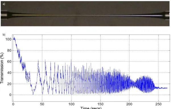
firmly mounted fiber was observed. Tapering was immediately initiated using a customized software, and the corresponding power transmission was recorded in-situ. From the transmission spectrum one can be able to distinguish between a lossy and an adiabatic tapering as shown in figure 3.1.c).
Figure 3.1: (a) shows a schematic representation of our setup for silica fiber tapering, (b)is a picture of the tapering part of the setup, (c) shows the power transmission against tapering length of the silica fiber and (d) compares the power transmission before and after tapering.
Initially, the fiber comprises of a single mode core-cladding guided light. How-ever, upon tapering down to certain diameters, the core eventually disappeared leaving a multi mode air-clad silica fiber (remember as mentioned earlier the core diameter of a tapered fiber decreases by the same amount as the whole fiber). Af-ter some further tapering, a single mode air-cladding guided fiber was obtained. Figure 3.1.d) shows the difference in transmission before and after tapering. It can be clearly seen that an adiabatic low loss tapering was successfully obtained.
3.1.2
Direct tapering of chalcogenide materials
After a successful adiabatic tapering of the silica fiber (with an air-cladding guided single mode), using a blade (Ideal DualScribe S90R) placed right at the center of the tapered silica fiber, the fiber was precisely cleaved under a microscope into approximately two equal halves. The successfully cleaved silica fibers were pulled apart using the motorized stage(Figure 3.2 a) 2) to provide enough space for chalcogenide feeding. Using a setup as shown in Figure 3.2 a), bulk chalcogenide on a glass slide was placed right in between the cleaved fibers ( Figure 3.2 a) 4 and 5), both the cleaved fbers and the bulk chalcogenide were enclosed by a homemade electrical heater ( Figure 3.2 a) 1), which provides enough heat to melt the bulk chalcogenide glass.
Figure (3.2, b)) is the home made electrical heater used for melting chalco-genide glasses. And c) shows the corresponding temperature variation as a func-tion of voltage. The heater was customized to have a saturafunc-tion at 140 V, where any further increase in voltage will be automatically limited to the melting tem-perature of the chalcogenide materials.
Figure 3.2: a) Shows the setup used for direct tapering of chalcogenide materi-als, where 1 is the home made electrical heater, 2 is the motorized stage/clamp upon which the silica fiber was mounted and held firmly on either sides, 3 is a microscope for insitu observation of the tapering process, 4 is a glass slide for chalcogenide feeding and 5 is the bulk chalcogenide. b) 1 is the home made elec-trical heater which was used to melt the chalcogenide glasses and c) shows the corresponding temperature of the homemade electrical heater at certain voltages.
Figure 3.3: a) and b) shows the initial feeding of molten chalcogenide upon the tip of tapered silica fiber.
After we have everything set as discussed, we then turn on the homemade electrical heater and wait for a couple of minutes for the chalcogenide to melt. Once chalcogenide is in the molten state, it can be transferred to both tips of the cleaved tapered silica fibers, by simply dipping the tapered silica tips one at a time into the molten chalcogenide and pulling it (as shown in Figure 3.3 a) and b)).
By bringing both chalcogenide fed tips into contact with each other, the molten chalcogenide at the two tips merges (Figure 3.4 a)). At this moment, we wait a little while for the chalcogenide to have a smooth distribution and stabilise
Figure 3.4: a) shows chalcogenide fed between the two tips of the tapered silica fiber by simply bringing both tips into contact. b) A smooth distribution and stabilization of chalcogenide between the tips and c) tapering begins by simply pulling the fibers apart.
between the tips (Figure 3.4 b)). Once that is achieved, we begin tapering of chalcogenide by cautiously pulling it apart using the motorized stage(Figure 3.4 c) ).
3.1.3
Results and discussion
Chalcogenide materials (As2Se3 and As2S3) were successfully tapered
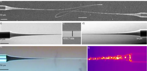
adia-batically with tapered waist diameter as low as sub-micron as shown in Fig-ure 3.5. a) and b) shows an adiabatically tapered chalcogenide fibers, and c) shows sub micron diameter adiabatically tapered chalcogenide fiber. This strongly demonstrates the remarkable ability of the technique to directly fabri-cate nanowires/nanofibers from a bulk material.
Figure 3.5: a), b) and d)shows an adiabatically tapered chalcogenide fibers. c) Sub micron diameter adiabatically tapered chalcogenide fiber, e) and f) are the corresponding optical microscopic image and thermal camera image.
We obtained a broadband transmission for the tapered ChG fiber (as shown in Figure 3.6), which was drawn until we reached single mode regime at a nanoscale waist diameter. Figure 3.7 compares the transmission spectrum of silica fiber before and after tapering, and that of tapered chalcogenide fiber. The total insertion loss was 21.1 dB, which was the sum of 6.4 dB silica to silica mechanical coupling and propagation loss, 0.6 dB silica fiber tapering loss, 1 dB Fresnel loss for both ChG/silica interface, 9.1 dB ChG tapering loss, and 4 dB loss due to cleaving and mode mismatch. Most of the loss (∼ 14.1 dB) was caused by the processes after silica fiber tapering, which was observed to be at least 8 dB for the best case. Starting ChG fiber tapering with smaller diameter silica tips (D < 20µm) is more favorable for adiabatic transition of the cladding guided modes, and reducing mode mismatch. The ChG fiber tapering loss includes losses due to nonadiabaticity, surface scattering, and Rayleigh scattering due to density fluctuations caused by different evaporating rates for As and Se, changing stoichiometry of the glass. In principle, angle cleaved silica fiber tips can eliminate the Fresnel losses, and tapering under inert gas atmosphere can reduce oxidation effects degrading ChGs.