Development and evaluation of inter-query optimization heuristics in database systems

к 85

Ш Ѳ 6

::íÍ?í;Cí ζ m , .^5 í i | W í ^ T i «

»İl'âtA' i» p4 »iW -^ > ‘ Íi/ » p-‘...<Ufr<r V ^ W km «W ·«' «W M '^ V *· a» « a· '•••'WV* >é4^4«

Й Р Т М Ш Ш ΐΐ.® іЦ%ТД ? w

^ - 'ί'· ν . · . -.>··; '. fiil · ίν . 'f c ;p v \:, > ; > > , · * . Л-'Ш.·! •,.i'î» .«· / , т . - . . ; , : г і; . - , - , ѵ я 'Ѵ * . · '? ‘Jw.U ;· J liwTÜ JvaiJlS'J Í • V'·· ;:^ '

áí;^¿!Í¿ví.ói^í-> .' ;? ..·. '•(К.ѵ‘ ѵ> ‘ '■^г. -Ѵ> '?*;V>Ï г к » .'..■-'«i γ \ ■^?а.ÿï/_ Г; лЧ. ·■··»г: .; ·■». . ·ι*·ϊ*,·3 ^ " y ”e l ¿ V i « г ^ '^ л л . u' 'а ^ '* и . У ^’ ^ ^ ϊ ^ ί · . ΐ ν ΐι·ι·*»..* ·|* <ί 'ч і ’ ѵ' ы и , ί ^ ¿ * m . m , >·*'' - . 'л m .· . » «· m , ..Ч . V s: а - - . · - а і’ч .i'··;. *■ ' і·^ .' ·* : ^ ч ч V '>.■,'/ν’· ‘і ■ - ѴѵѴ* ..г · - - ■ — Л1аа»и. ·;. « ^ ί:-'Τ^νϊ ?" *

DEV ELO PM ENT AND EVALUATION OF

INTER-Q UERY O PTIM IZATIO N HEURISTICS

IN DATABASE SYSTEM S

A THESIS

SUBMITTED TO THE DEPARTMENT OF COMPUTER

ENGINEERING AND INFORMATION SCIENCE

AND THE INSTITUTE OF ENGINEERING AND SCIENCE

OF BiLKENT UNIVERSITY

IN PARTIAL FULFILLMENT OF THE REQUIREMENTS

FOR THE DEGREE OF

MASTER OF SCIENCE

By

Yigil Kiilaba§

January, 1996

— ... larcfnidi,: ia

G2h ^ 6 . 3

■ Ь З

K S5

I certify that I have read this thesis and that in my opinion it is fully adequate, in scope and in quality, as a thesis for the degree o f Master o f Science.

Asst. Prof, özgür Ulusoy (Advisor)

I certify that I have read this thesis and that in my opinion it is fully adequate, in scope and in quality, as a thesis for the degree o f Master o f Science.

Assoc. Prof Cevdet Aykanat

I certify that I have read this thesis and that in my opinion it is fully adequate, in scope and in quality, as a thesis for the degree o f Master o f Science.

Approved for the Institute o f Engineering and Science:

Prof Mehmet itâray Director o f the Institute

ABSTRACT

DEVELOPMENT AND EVALUATION OF

INTER-QUERY OPTIMIZATION HEURISTICS

IN DATABASE SYSTEMS

Yiğit Kulabaş

M.S. in Computer Engineering and Infomiation Science

Advisor: Asst. Prof. Özgür Ulusoy

Janiiaiy, 1996

In a multi-user database system multiple queries can be issued by different users at about the same time. These queries may have some common operations and/or common relations to process. In our work, we have developed some inter-query optimization heuristics for improving the performance by exploiting the common relations within the queries. We have focused mostly on the join operation, with the build and probe phases. Some o f the proposed heuristics are for the build phase, some for the probe phase, and finally some for the memory flush operation. The performance o f the proposed heuristics is studied using a simple simulation model. We show that the heuristics can provide significant performance improvements compared to conventional scheduling methods for different workloads.

Keywords: Inter-query optimization, join operation with build and probe phases, memory flush operation.

ÖZET

VERÎTABANI SİSTEMLERİNDE

SORGULARARASI OPTİMİZASYON METODLARININ

GELİŞTİRİLMESİ VE İNCELENMESİ

Yiğit Kıılabaş

Bilgisayar ve Enformatik Mühendisliği Bölümü - Yüksek Lisans

Danışman : Yrd. Doç.Özgür Ulusoy

Oeak 1996

Çok kullanıcılı veri tabanı sistemlerinde, yakın zamanlı olarak birden fazla sorgunun, değişik kullanıcılar tarafından sisteme yüklenmesi sıkça rastlanan bir durumdur. Bu sorgular ortak işlem ve/veya verilere sahip olabilirler. Çalışmamızda, bu ortak işlem ya da verilerin, sorgular tarafından paylaşılması amacıyla bazı sorgulararası en iyileme (optimizasyon) teknikleri geliştirmiş bulunmaktayız. Bu çalışmalar sırasında daha çok birleştirme (jo'''') işlemine odaklandık. Birleştirme işleminde ise şekil olarak dağıtım kodlaması (haslı) tekniğini kullandık. Geliştirilen metodların bir kısmı dağıtım kod tablolarının oluşturulması, bir kısmı bu tabloların sorgulanması, bir kısmı ise belleğin verimli olarak kullanılmasını sağlamaktadır. Çalışma kapsamında ayrıca bu metodların performansları bir benzetim modelinin üzerinde karşılaştırılmıştır. Karşılaştırmalar sonucunda en çok dikkat çeken nokta ise, geliştirilen bütün tekniklerin, sorguların birer birer ele alınması tekniğine göre oldukça önemli üstünlükler göstermesi olmuştur.

Anahlar Kelimeler: Sorgulararası en iyileme, birleştirme işlemi, inşa-etme aşaması, sorgulama aşaması, bellek temizleme aşaması.

ACKNOWLEDGEMENTS

I am very grateful to my advisor Asst, Prof Özgür Ulusoy for his guidance, suggestions, and encouragement throughout the development o f this thesis. I would like to thank Prof Erol Arkım and Assoc. P ro f Cevdet Aykanat for reading and commenting on the thesis.

Contents

1. Introduction

1

1.1. Overview of Multi-Queiy Environments

1

1.1.1. Intra-Query Parallelism vs. Inter-Queiy Parallelism 2

1. 1.1.1. 1 ntra-Query Parallelism 2

1.1.1.1.1. Pipelined Intra-Query Parallelism 2 1. 1. 1. 12. Partitioned Intra-Query Parallelism 3

1. 11. 2. Inter-Query Parallelism 3

1.1.2. Inter-Queiy Parallelism and Relational Operations 3

1.2. Overview of the Thesis

4

1.3. Related Work

5

2. Inter-Query Optimization

2.1. Which Relation to Build?

2.2. How and When to Probe?

2.3. Which Relation to Flush?

7

8

10

14

3. Algorithms

3.1. Main Algorithm

3.2. Main Outline According to Probe Heuristics

.3.2.1. Immediate Probe 3.2.2. Total Probe 3.2.3. Partial Probe

3.3. Initialization Session

3.4. Build Algorithms

3.4.1. Build by Largest Number o f Tuples that will Probe 3.4.2. Highest Number o f Relations Interacted with 3.4.3. Smallest Size 18 19 19 19

20

21

22

2 4 2 4 2 6 2 8 VI

3.5. Probe Phase

3.6. Flush Algorithms

3.6.1. Largest Sized Relation 3.6.2. Flush by Join-Set 3.6.3. Consecutive Flush

29

32

32

35

37

4. Simulation Model

40

5. Performance Results

5.1. Comparison of the Probe Heuristics

5.2. Comparison of the Build Heuristics

43

43

45

6. Conclusion and Future Work

47

7. References

48

List o f Figures

Figure I : Comparison of the Probe Heuristics - Perfonnance

43

Figure 2: Comparison of the Probe/Flush Heuristics - Performance

44

Figure 3; Comparison of the Probe Heuristics - Utilization

45

Figure 4: Comparison of the Flush Heuristics - Utilization

45

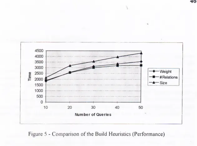
Figure 5: Comparison of the Build Heuristics - Perfonnance

46

Figure 6: Comparison of the Build Heuristics - Memoiy Utilization

46

List o f T ables

Table I: Simulation Model Parameters

Table 2: CPU costs of Some Operations

40

40

1. Introduction

We start this chapter with a brief introduction to the concepts in Multi-Query Environments, Query Scheduling Optimization, Intra-Query Parallelism, Inter-Query Parallelism, and Sharing Relational Operations. Following this general introduction, we provide a brief overview o f the thesis topic, along with the related work and the general organization o f the thesis.

1.1. Overview of Multi-Query Environments

During the last decade, there have been significant enhancements in the performance o f computer systems. The processor speed and the capacity o f main memory and secondary storage devices have steadily increased. Symmetric multiprocessing

technology, clustering technology, and parallel processing technology have

continuously been improved. These enhancements have also enforced improvements in the database technology. The leading database vendors have developed uniprocessor, multiprocessor, clustered, and parallel versions o f their DBMS’s. These versions have continuously been enhanced to have better performance.

An important part o f the workload for the database systems consists o f resource­ intensive read-only queries. For this reason, one o f the main factors that the performance depends on, is query scheduling. To optimize the scheduling o f queries in terms o f the response time, various algorithms have been developed. These algorithms mainly focused on intra-query parallelism. In other words, research on query scheduling has so far concentrated mainly on efficient processing o f single queries. However, an important property o f DBMS’s, regardless o f whether they are uniprocesor, multiprocessor, clustered, or parallel systems, in general they are multi­ user systems. In a multi-user system, multiple queries can be delivered by different users at the same time. A multi-user environment leads to “multi-query” executions, and to optimize query scheduling in such environments, the focus should not be only on “single-queiy” execution but also on “multi-quei-y” execution.

In a multi-query environment, quite often the same relation is a part o f several queries. When the queries are optimized only by the single-queiy manner, such relations are processed multiple times, since the queries are scheduled independently. If these relations could be shared between concurrently executing queries, they would have to be processed only once.

A multi-query scheduling method can optimize a set o f queries together, by identifying common relations in the set and scheduling them in such a way that the repeated processing o f the common relations is avoided. Therefore, the total execution time o f queries will decrease.

This thesis is focused on efficient scheduling o f “multi-queries”. Several scheduling algorithms are presented which can be used to take advantage o f sharing o f relations among a set o f queries. The aim is to optimize query scheduling in multi-user environments. The general information about the thesis can be found in Section 1.2. Before the overview, let us go over the parallelism concepts used in query scheduling.

1.1.1. Intra-Query Parallelism vs. Inter-Query Parallelism

Various queiy scheduling techniques based on parallelising query executions, have been developed. The focus in these techniques have basically been on the parallel execution o f a single queiy at a time. This type o f parallel execution is called “intra­ query” parallelism.

1.1.1.1. Intra-Query Parallelism:

This type o f parallelism is used in most o f the parallel machines, and parallel DBM S’s. There are two types o f intra-query parallelism:

- Pipelined Intra-Queiy Parallelism - Partitioned Intra-Query Parallelism

1.1.1.1.1. Pipelined Intra-Query Parallelism:

Queries that require multiple relational operations can be parallelised by the “pipeline” version. In this type o f scheduling, the operations are classified on the basis o f whether they are dependent or independent. The dependent operations use the output o f the other operations (e.g., sorts, aggregation).

This type o f parallelism benefits in OLCP (On-line Complex Processing) and DSS (Decision Support Systems) response times and can be used on any type o f multi­ processor machines 111.

1.1.1.1.2. Partitioned Intra-Qiiei^ Parallelism:

Any type o f quei7 can be parallelised by this method since the parallelism is achieved by data partitioning. In this type o f scheduling, database tables are partitioned and spread across multiple disks.

This type o f parallelism provides a high degree o f scalability when searching database tables, benefits DSS processing o f large tables and is only available on parallel (shared- nothing) machines [1].

1.1.1.2 Inter-Quei7 Parallelism:

This method deals with the scheduling o f more than one queiy at a time. In this type o f scheduling, multiple threads are used for execution o f each query. Multiple threads may execute on multiple processors. There is a significant benefit in reducing OLTP response times.

In the literature, the term “inter-query parallelism” is mostly used to refer to the “independent” processing o f multi-queries as multi-threads. In this thesis, we deal with the “dependency” o f the multi-queries, which is another side o f the inter-query parallelism [1].

1.1.2. Inter-Query Parallelism and Relational Operations

Inter-queiy parallelism can be applied on any type o f relational operations. It tries to achieve the following goal: get the information in the relations into the main memory and complete the operation as quickly as possible. Therefore, efficient memory management is one o f the most important requirements in query scheduling. Inter­ query parallelism can optimize the memory usage by sharing common tables between different operations o f different queries.

Among all relational operations, the join operation is distinguished by its complexity. It is the most expensive relational operation in terms o f the amount o f system resources required. Many algorithms have been developed to eliminate this complexity; namely traditional nested loops, hashing techniques, sort-merge techniques, and their mixtures. All these algorithms have both serial and parallel versions. It has been shown that hash- based join algorithms outperform the others in most environments. There are also different versions o f the hash join algorithms. One o f the most commonly used one is the hybrid-hash join algorithm. In this thesis our discussions will basically involve this algorithm.

The hybrid-hash join algorithm executes in two phases, called “Build” and “Probe” . In the first phase, the smaller relation is scanned and an in-memory hash table is constructed by hashing each tuple on the join attribute. In the second phase, the outer relation is scanned and hash values o f the tuples are used to probe the hash table to test for matches. The matched tuples are joined. There is a partial order defined on these two phases. The probe phase cannot begin until the build phase is completed [2].

Although sharing in multi-query environments is applicable for any type o f query operations, the focus in this thesis will be on the join operation.

1.2. Overview of the Thesis

This thesis presents several scheduling algorithms that can be used to exploit the sharing o f relations for batches o f queries.

In a multi-user database system, the queries delivered to the same system, by different users at about the same time, can include the same relations, operations, or even the same total query. As an example consider an Airline Database. There can be lots o f agencies, and other users entering exactly the same query: “Flights from New York to Miami on Dec 27, 1995” at about the same time. Or, think o f a similar example, this time the queries entered about the same time are not exactly the same but they use the same relations: user-1 “Flights from New York to Miami on Dec 27, 1995”, user-2 “Flights from New York to San Francisco on Dec 27, 1995”.

If the queries delivered within a certain time period are not considered as a batch, the potential o f sharing some operations and relations can not be exploited. This is the point that shows the importance o f inter-quei^ optimization for the performance enhancements, and resource utilization. However, this topic has been considered in just a few works as explained in Section 1.3. The significance o f inter-query optimization and the lack o f enough research works in this topic have been the basic motivations o f the thesis.

An ideal multi-query scheduling method would optimize a set o f queries together and minimize the total execution time. The conventional multi-query scheduling corresponds to scheduling queries independently. The scheduler allows the maximum possible number o f queries to run together with no consideration for the sharing o f relations.

The optimum exhaustive sharing algorithm has a huge time complexity: n!.2".m!, where n is the total number o f relations, and m is the numbei· o f relations in the memory. Here n! is the complexity o f selecting an ordering o f the queries, 2" is the number o f choices to select probe/build relations, and m! is the complexity o f determining the order in which relations are flushed from the memory [3]. Therefore, using the exhaustive algorithm is not feasible. Heuristic algorithms need to be developed to provide efficient sharing o f relations in a batch o f queries. The thesis provides such heuristics and presents their performance results obtained in a simulation environment.

For the sake o f simplicity, some assumptions have been made in developing and testing the heuristics. A uniprocessor, multi-user database system has been chosen as the query execution environment. Due to its large time complexity, the join operation has been chosen to apply the inter-queiy optimization, although it is applicable to any kind o f operations. For the implementation o f the join operation, the Hybrid-Hash Join Algorithm has been used. All the algorithms have been designed to optimize the execution time o f the build and probe phases o f the hybrid hash join, and the memory flush operation, by exploiting the share o f the common relations. All the queries are assumed to be single-join queries; i.e. each query consists o f a join o f two relations. A full queiy optimization will be possible when the intra-query and inter-query optimization techniques are used together. In this thesis, we ignore the application o f intra-queiy techniques as our focus is on inter-query processing.

The remainder o f the thesis is organized as follows. In the second chapter, inter-query optimization will be discussed. The ideas behind developing the heuristics will be explained in detail. In the third chapter, the scheduling algorithms based on the proposed heuristics will be demonstrated. Each algorithm will be explained in detail, and related examples will be given. The fourth chapter is devoted to the simulation results. The performance results o f the algorithms will be compared in this chapter. The last chapter concludes the thesis and provides some suggestions for the future work.

1.3 Related Work

The work on the optimization o f queries have mostly been provided for single query scheduling. The optimization techniques have first begun with the simple, basic queries |4| and extended to larger and more complex queries [5] [6] [7] [8] [9].

For multi-query scheduling, we noticed that the number o f related works is very few. One o f these works is [10], which examines the effect o f different memory allocation schemes. But this is a very preliminary study that can not answer important scheduling policy questions. There are some query-language-level optimization research conducted for multi-query environment [11] [12] [13] [14].

One o f the studies that deals with multi-query optimization at the individual query operator level is the inspiration o f this thesis [3]. In this study, the hybrid-hash join with the build and probe phases, is the operation that is focused on. In this paper, there are several heuristics proposed for improving the average response time o f multiple queries. Our work considers a similar execution environment and has the same scheduling goal. We have developed some more heuristics for the build and flush phases o f the join operation. We have also developed different probe heuristics. In [3] no alternatives are provided for the probe phase.

When developing new techniques for the join operation, we have had an extensive research on the join optimization [15] [16] [17] [18] [19] [20] [21] [22] [23] [24] [25] [26] [27]. Some o f these papers deal with different join techniques, some with hashing details in the join environment, and some with CPU, disk and memory usage o f the join operation.

2. Inter-Query Optimization

In a set o f queries, if several joins involve the same relation, the hash table for this relation can be shared. Here is a simple set as an example.

JOIN(X,Y), JOIN(X,Z).

For both joins, we have two phases: build the hash table o f one o f the relations ( in most cases, the small one), probe the hash table with the other relation. Here the relation to be shared is X, and relations Y and Z will share the hash table o f X to probe.

The sharing we just considered has two significant impacts on the efficiency o f query execution. Since the built relation is scanned once, the total execution time is reduced. (If the two operations were handled separately, hash tables o f two relations would have to be built, and the scan time would be doubled.) Another impact on the performance is that, since only one table is built, there will be a considerable saving in the memory usage.

As could easily be noticed, in the case o f two queries it is straightforward to determine which relation should be selected to build and which one to probe. This decision does not require the involvement o f complex algorithms.

Consider another set o f queries:

JOIN(X,Y), JOIN(X,Z), JOIN(X,T), JOIN(T,Z), JOIN(T,A), JOIN(Y,Z), JOIN(A,Y) In this case, the queries involve relation Y 3 times, relation X 3 times, relation Z 3 times, relation T 3 times, and finally relation A 2 times. Which relations should be built? Relation Y, X, Z, or T? Or even relation A? Let Y be the built relation and X, Z and A make the probes. After this processing (i.e. the probes to the hash table o f relation Y are finalized ), we are left with the requirement to process X 2 times, Z 2 times, T 3 times, and A 1 time. Let T be selected to be built and the probes are made. We are left with the processing requirements o f X and Z 1 time. Is this a good solution? If Y and T had been built at the same time, and the probes would have followed them, would the total execution time be shorter? Would Y and T fit into memory at the same time‘s If T and A together fit into memory, would it be more efficient to build them both? After T and A are built, we still have to build X, Y, or Z, but none o f them fits into memory; so, which relation should we flush from the memory? In selecting a relation to build, what criteria need to be considered? Many more similar questions can be asked. This simple example clearly illustrates the requirement for the optimization algorithms for the shared relations in processing the join operations.

8

Three basic questions are involved in inter-query optimization: - Which relation to build?

- How and when to probe? - Which relation to flush?

2.1. Which Relation to Build?

There can be many different considerations in detecting the relation to be built. Again, let us consider an example:

Set o f Queries:

J01N(A,B), J01N(A,C), JOIN(B,C), JOIN(B,D) with the following sizes

Relation A: 20 pages. Relation B: 40 pages, Relation C: 10 pages, Relation D: 20 pages.

A number o f heuristics can be considered in determining the built relation:

Heiirislic I - Highest Number o f Relalio/is Inleracled with:

In the example, A and C join with 2 relations, B with 3 relations, while D joins with only one relation. According to this heuristic, for this example, relation B is selected to be built. Phase I Number o f Relations Interacted with Phase 2 Number o f Relations Interacted with

Relation A: 2 - ( B , C ) probe 1 - ( C ) build

Relation B: 3 - ( A , C , D ) build 0

Relation C: 2 - ( A, B ) probe l - ( A ) probe

Relation D: 1 - ( B ) probe 0

When the hash table o f relation B is formed, the three relations that B joins, namely A, C and D can probe the table at the same time. As a result o f these probes, the queries JOIN(A,B), JOIN(B,C), J01N(B,D) are processed (End o f Phase I). Only the query JOIN(A,C) remains unprocessed. At this stage (Phase 2), B and D will have the value 0 (i.e., there is no join operation that uses these relations left), while A and C have 1. One o f the relations will be built, the other one will probe and the remaining query, J01N(A,C) will be processed,

The aim o f using this heuristic is to build the relation that will be probed with the maximum number o f relations. If we assume that each join query is assumed to be submitted by a different user, by this heuristic, after the build and probe phases, the highest number o f users will get the results for their queries.

Heuristic 2 - Largest Number o f Tuples that 'will Probe[3]:

Let’s define the Weight o f a Relation X as the total size o f the relations that Relation X joins with. In the example given above, we have the following weights; A 50 (40+10), B 50 ( 20+20+10), C 60 (40+20), and D 40. As the first step, C is chosen to be built as its weight is larger than the others. If we use Heuristic 2, C will be built as shown below.

Phase I

Weight

Relation A: 50 - fSize(B) + Size(C), 40+10) probe

Relation B: 50 - (Size(A) + Size(C) + Size(D), 20+10+20) probe

Relation C: 60 - (SizefA) + Size(B), 40+20) build

Relation D: 40 - (Size(B), 40) N/A

A and B will make the probes and the queries J01N(A,C) and JOIN(B,C) will be processed first. In the second phase, we have:

Relation A Relation B Relation C Relation D Phase 2 Weight - Heuristic 2 40 - iS ize (B ), 40) 40 - (Size(A) + Size(D), 20+20) 0 40 - (Size(B), 40) Heuristic 1 1 -( B ) 2 -( A ,D ) 0

1 - (B)

All the joins o f C are processed and C has a weight 0, while A, B, and D has the weight 40. If we apply only Heuristic 2, any o f three relations A, B and D is selected to be built. But, if we also consider Heuristic 7, B will be the one to be built since it interacts with 2 relations while the others interact with only one. After B is built, the remaining queries will be processed.

The aim o f using this parameter is similar to that o f Heuristic 7, but in this case, the relative sizes o f relations are also important. There is a subtle memory utilization: the larger relations are enforced to make probes and leave the memory as soon as possible. Therefore besides response times, the memoiy utilization is also considered.

10

This heuristic is directly related with the size o f the relations. The relation with the smallest size is selected to build. In the given example the sizes o f A, B, C, and D are respectively 20, 40, 10, and 20. Thus, C will be the built relation. A and B will make the probes. Then A or D is built. The built one will be probed by B. Finally, the relation A or D that was not built in the previous step, will be built and be probed by B. Here, the only performance consideration is the savings in memory utilization.

It is also possible that these three heuristics can be used together. Consider the following types o f algorithms:

M ixed Algorithms:

Various combinations o f heuristics could be considered in scheduling algorithms. Some examples can be:

weight / size, (Heuristic 2 / Heuristic i )

number o f relation probes / size, (Heuristic I / Heuristic 3)

number o f relation probes x weight,

c 1 X number o f relation probes + c2 x weight + c3 x size (for some constant cl,c2,c3 values)

Heuristic 3

-

Smallest Size:

etc.

Cascaded A Igorithins:

A possible scheduling algorithm can be:

If the weights o f two relations are the same, use the number o f relations heuristic. If they are also the same, build the small sized relation.

2.2. How and When to Probe?

The hash tables o f the built relations are probed by the other relations. But there can also be different considerations about the probing.

11

The probing can be done immediately after the relation is built. While explaining the Building Heuristics, this type o f probing has been assumed.

Let us consider the same example with a limitation in the memory size: Set o f Queries:

JOIN(A,B), JOIN(A,C), JOIN(B,C), JOIN(B,D) with the following sizes

Relation A: 20 pages, Relation B: 40 pages, Relation C: 10 pages. Relation D: 20 pages, and the memoiy size is 50 pages.

If we use Heuristic 1 for choosing the relation to build, as you could remember the order o f the built relations will be B and A (or C) . If we use Heuristic 4 for probing after the hash table o f B is built, it will be immediately probed by A, C, and D. And as a result, JOIN(A,B), JOIN(B,C) and JOIN(B,D) will be processed. After probes are completed, the hash table o f B will not be used again, so it is flushed from the memory. Then, the hash table for A is formed and JOIN(A,C) is processed by probing the hash table o f A with C.

He m i Stic 4 - 1m mediate Probing:

This type o f probing has some advantages as well as some disadvantages. One o f the advantages arises from the timely response given to some o f the users. The user gets his/her answer immediately after one o f the relations in his/her queiy is built. Another advantage is related to the memory management; the memory contains at most one hash table and is always available for other operations.

The disadvantage arises from the optimization point o f view. For the above case, B is probed by A, C, and D. After this, the hash table for A is built and is probed by C. If the hash tables o f both A and B were available at the same time, the hash values for C would be calculated only once and C would probe both tables at the same time. (Here we assume that the join attributes o f C are the same in both queries.) With Heuristic 4,

we will not be able to take this advantage and the processing time will increase. Another disadvantage arises again from the user side. It has been mentioned as an advantage that, some o f the users get their results as soon as a hash table related to their queiy is obtained. But, the owner o f the last handled queiy will wait until all the previous queries are processed.

12

Henri Stic 5 - Probe with No Need fo r a Flush:

The probing phase can wait until all the relations are built. This can be achieved if the memory is large enough to contain all the hash tables o f the built relations.

Let us use Heuristic 3 for choosing which relation to build. As you could remember the order o f the relations to build will be C, A and D. And, let us use Heuristic 5 for probing. C will use 10 pages o f the memory, while A and D use 20 pages each. And as a result, the memory will be totally occupied. After this, all the probes will be done. This heuristic is not complete, because most o f the time the memory is not large enough to contain all the hash tables o f the built relations. The Heuristics 7, 9 and 10

are alternatives to handle this case, and they all make use o f Heuristic 5 for the case that the memoi7 is large enough to handle all the hash tables. Before discussing those heuristics, let us focus on another issue:

Heuristic 6 - Jh-obe while Building:

When there are more than one relation built in the memoiy, we can have the following situation : the relation that will be built next can also be able to probe one or more hash tables residing in the memory.

Consider again the same example. By using Heuristic 3 for choosing which relation to build, we will have the order o f the built relations as C, A, and D. First C is built. After that, it is time for A to be built. While building the hash table o f A, the hash values o f A can also probe C and finalize JOIN(A,C). If this is not done, following the build phase o f all relations, the hash values o f A will again be computed to probe C.

After A is built, the hash table for D is built. And finally B will probe all the built relations A, C, and D; and J01N(A,B), .I01N(B,C), JOIN(B,D) are processed.

So far, there was no need for a flush to occur, as it was assumed that the amount o f memory is large enough. Let us have a more complex example for the rest o f heuristics with flush operation:

Example 2:

JOIN(A,B), JOIN(A,C), J01N(B,C), JOIN(B,D), JOIN(A,E), JOIN(C, E) with the following sizes

Relation A: 20 pages. Relation B: 40 pages. Relation C: 10 pages. Relation D: 20 pages. Relation E: 30 pages

13

The probing phase can wait until there is no place in the memory for the hash table o f the next relation to be built. To build the next relation, we need to flush at least one hash table o f a relation from the memory.

Let us use a cascading algorithm for choosing the order o f the relations to build; Apply

Heuristic 7; if the values obtained for some relations are the same, apply Heuristic 2; if some relations still have the same values for Heuristic 2 , apply Heuristic 3.

We have the following values for each o f the relations for the three heuristics:

Heuristic 7 - Partial Probe:

Heuristic 1 Heuristic 2 Heuristic 3

Relation A: 3 - (B, C, E) 80 - (Size(B)+Size(C )+Size(D ),40+10+30) 20

Relation B: 3 - (A, C, D) 50 - (Size(A)+Size(C)+Size(D),20+10+20) 40

Relation C: 3 - (A, B, E) 90 - (Size(A)+Size(B)+Size(E), 20+40+30) 10

Relation D: 1 -(B) 40 - (Size(B), 40) 20

Relation E: 2 -(A, C) 30 - (Size(A)+Size(C), 20+10) 30

And the order o f relations for being built will be: C, A and D. We have a memory o f 40 pages. When C is build, 30 pages o f memory is left. The next relation A is 20 pages. Therefore, we have enough space for A. A will be built using Heuristic 6: it will probe C while being built and finalize the queiy JOIN(A,C). After A is built, the amount o f left memoiy is 10 pages. When it is time to build D, there is no enough space for this relation as its size is 20 pages and there is only 10 pages o f available memory. Therefore, we have to flush relations till there is enough space for Relation D. If A is flushed, the available memory size will increase to 30 pages which is enough for Relation D. So, let us flush A.

Before flushing A, relations B and E will probe the hash table o f A. Both B and E will also need to probe the hash table o f C. To probe A, the hash values o f B and E will be computed and to probe C at a later time, recalculating these values will only be a waste o f time. So, the probing o f A and C by B and E will be done at the same time. This can be specified as another heuristic:

Heuristic b - Probe More than one Hash Table: If the probing o f different hash tables at the same time is possible, finalize the probes to avoid recalculating the hash values at a later time.

By using this heuristic, the queries .101N(A,B), JOIN(B,C), JOIN(A,E), JOIN(C,E) will be finalized at the same time. After this, A will be flushed and then D will be built. C can also be flushed since there is no more relations to probe it. As the next step, B will probe D.

14

HeunsUc 9 - I^’lush All:

This heuristic works the same as Heuristic 7 until the flush time. When the flush o f a relation is needed, all the relations in the memory are flushed.

Let the order o f relations for being built be; C, D, and A. We have a memory o f 40 pages. When C is built, 30 pages o f memory is left. The next relation D is 20 pages. That is to say we have enough space for D. D will be built, and since there is no join operation on D and C, Heurisiic 6 is not applicable at this step. After D is built, the amount o f available memory is 10 pages. When it is time to build A, there is no enough space for this relation as its size is 20 pages. So we have to flush some relations. By this heuristic all the relations are flushed. Before the flush o f D, it is probed by B, B probes C at the same time using Heuristic H. Before the flush o f C it is also probed by A and E. After the flush operations, JOIN(A,C), JOIN(B,C), JOIN(B,D), JOIN(C,E) queries are completed and the whole memory is available. As the next step, A is built and it is probed by B and E. As a result, all the queries are completed.

Let us now consider the sequence o f operations that uses the same build order and performs probing by using Heuristic ~ The workflow is exactly the same until the need for a flush. According to Heuristic ", flushing only D is enough. When D is flushed, the available memory size will increase to 30 pages and 20 paged A can fit into the memory. Before the flush, D is probed by B. B probes C at the same time by

Heuristic 8. The queries J01N(B,C), J01N(B,D) are processed. After the probe o f B, D is flushed. C still remains in the memoiy, since the other probes o f C, namely probing by A and E are not completed. The next step is building relation A. A probes C during the building phase using Heuristic 6. Then E probes A and C at the same time {Heuristic 8), and A is also probed by B. All the queries are processed.

Heuristic 9 has a disadvantage over Heuristic ". The disadvantage arises from not being able to use Heuristic 8. For the above example, using Heuristic 9 causes the hash values o f E to be processed twice. In veiy complex queiy environments, i.e., real life examples with hundreds o f relations, this re-processing can cause an important add-on to the query time. Therefore, Heuristic can be expected to perform better than

Heuristic 9.

2.3. Which Relation to Flush?

After deciding which relation to build, the next step is to build the hash table o f the selected relation, if o f course there is enough space in the memory for the hash table. If there is a memoiy limitation, then some o f the relations should be flushed out o f the memoiy.

15

Here emerges another question. If there are more than one relation in the memory, which relation should we flush? Flushing all the relations in the memory vs. flushing until there is enough space for the next relation to be built was discussed in Section 2.3. If the second alternative is used, what should be done to detect which relation to flush? This new issue is also another important criteria related to query optimization. Let us again use Example 2 with the build criteria used in Heuristic 7. The flow o f the query scheduling was as follows:

The order o f relations for being built are: C, A and D. We have a memory o f 40 pages. When C is build, 30 pages o f memory is left. The next relation A is 20 pages. That is to .say we have enough space fo r A. A will he built as in Heuristic 6: it will probe C while being built and finalize the query J01N(A,C). After A is built, the amount o f memory left is 10 pages. When it is time to build D, there is no enough space fo r this relation with its size o f 20 pages and 10 pages o f available memory. So, we have to flu.sh relations till there is enough .space fo r Relation D.

Here comes the question: should we flush C or A?

Heuristic 10: Plush the Larger Sized Relation:

Relation A has a size o f 20 while C has 10. According to this heuristic A should be flushed first. When A is flushed, the available memory will increase to 30 pages which is enough for Relation D. So there is no need to flush C to build D.

Heuristic 11: l-lush According to the .loin Set o f the Next Relation to he Built:

Let us have another example. We have the relations with the following properties:

Number o f relations Join Set

Interacted (Relations Interacted with) Size

Relation A: 4 {B, C, E, G} 20 Relation B: 5 {A, C, D, F, G} 30 Relation C: 2 {A,B} 20 Relation D: 1 iB} 20 Relation E: 1 {A} 20 Relation F: 2 {B,G} 30 Relation G: J (A, B ,F} 20 M emoiy Size: 50

16

Let the order o f building the relations be : B, A, G.

Let us have the relations A and B in the memory. And it is time to build G. If we use

Heuristic 10, we will flush B. By this way, C and G will probe both A and B. D and F will probe B. After this, G will be built. Since there is no relation need to be built, the probes are completed. A will be probed by E, and G will be probed by F.

As you can notice, the hash values o f F are computed twice, once for probing B before its flush, and once for probing G. Instead o f flushing B, if we flush A all the hash values will be completed only once. Before the flush o f A, C and G will probe both A and B. A will also be probed by E. After this, G will be built. Then the probes are completed and F probes both B and G, and E probes B.

In Heuristic 11 , before selecting the relation to flush, the relations that are in the join set o f the next relation in the build queue, and the relations that are in the join set o f the relations in the memory are compared.

In the example, the next relation to build is G, with the join set {F}. The relations in the memory are A and B with the join sets o f {C, E, G} and {C, D, F, G ), respectively. The intersection o f the join sets o f A and G is empty set, while the intersection o f the join sets o f B and G is {F}. Since the number o f elements in the intersection set o f A and G, is less then the intersection set o f B and G, A will be flushed out o f the memory.

Before using this technique, some investigation should be done. For the above example, flushing either A or B is enough for G to be built. If we do not make any pre­ investigation, and directly use Heuristic 11, there w on’t be any advantage. For the above example, let the join sets be the same but the sizes be different. Let B be 40, A be 10 and G be 20. Here flushing only A, is not enough for G to be built. But if we directly use Heuristic 11, A will be flushed and after this since the memory is not enough for G, B will also be flushed before building G.

Heuristic 12 - Consider also the Next Hatch

While processing the last queries in a batch, the hash tables in the memory can also be used by the next batch. At the end o f the processing o f a batch o f queries, the probes to the in-memory relations will be completed, but the relations will not be flushed from the memoiy. When it is the time for the next batch, the in-memory relations will be assumed to be the first built relations.

17

Let us consider the first batch as the above group, we have A and G in the memory as the final step. Let us assume that without using this heuristic, the build queue o f the second batch is as follows: B, E, G. But by Heuristic 12, since G and A are already in the memory, the build queue will change according to the new weights without considering G and A.

18

3. Algorithms

Before discussing the algorithms, let us first go over some important data structures used. The queries are formed randomly. Each query is a row in the

query-table.

An

inter-relation table

is formed by using query-table. Before its usage let us give an example: R el-1 R e l-2 R1 R 2 R1 0 R 3 R1 R 2 1 0 R 4 R1 R 3 1 1 0 R 7 R 5 R 4 1 0 0 0 R 5 R 6 R 5 0 0 0 0 0 R 6 R 5 R 6 0 0 0 0 1 0 R 5 R 7 R 7 1 0 0 1 1 0 0 R1 R 7 R1 R 2 R 3 R 4 R 5 R 6 R 7 R 2 R 3 R 7 R 4 inter-relation table query-table

Inter-relation table is used in all the algorithms. At the initial state, this table shows whether there is a join operation between two relations. In the example, since there is a query as JO IN (R l,R2), the value in the inter-relation table for the cell R1-R2 is 1. In the same manner, since there is no join between R2-R4, the corresponding value in the inter-relation table is 0, Join is a commutative operation. For both JO IN (R l,R 2) and JO IN (R 2,Rl), the operation is completed by building either R1 or R2, and probing with the other one. For this reason, the corresponding value for R1-R2 in the inter­ relation table is set by one o f the mentioned joins.

Besides these two tables, we have some more tables that are algorithm specific. These tables are:

size-table: This table shows the size o f each relation. It is formed at the initialization part and is not changed by any algorithm ( i.e., it is a static table).

weight-table: This table shows the sum o f the sizes o f relations that a relation joins with. It is formed according to the join-table and continuously modified as the joins are completed.

winiber-of-relalions-table: This table shows the number o f relations that a relation joins with. This table is a dynamic table as weight-table and modified as the queries are

19

3.1. Main Algorithm

The main algorithm for the join operation is directly related with the probe phase. All the algorithms start with an

initialize

session. In this session, the tables are initialized. Then the queiy set is formed randomly by

gethatch.

Then the other parts o f the main algorithm

build-criteria, huUd, flush-criteria, probe

a n d t a k e place according to the probe workflow. Let us go into procedural details.

Build -criteria: This part is directly related with the build heuristic. Build: The main build phase.

Flush-Criteria: This part is directly related with the flush heuristic.

Probe: The main probe phase. As mentioned before, the probe heuristic forms the

main outline. This algorithm only deals with the probe details, not the heuristics.

Flush: The flush job is done in this phase.

The main algorithm without inter-relation optimization is as follows:

initialize

getbatch

fo r each Joit) query begin

build the hash table o f the first relation

probe the hash table with the hash values o f the other relation

flush

the hash table o f the relation from the memory

end

Since there is no optimization, the inter-relation table, weight-table, number-of- relations-table, build-criteria algorithm, and flush-criteria algorithm are not used. For each query one o f the relations is built, the other relation probes the hash table o f the built relation, and after the probe the hash table is flushed from the memory.

To see the outline o f the optimized version, let us first focus on the probe heuristics.

3.2. Main Outline According to Probe Heuristics

In this part only join heuristics will be discussed. The real join process will be described in detail in Section 3.5.

3.2.1. Immediate Probe

The probing can be done immediately after the relation is built as discussed in detail with Heuristic 4. The main algorithm now takes the following form:

20

initialize

gethatch

while there exist jo in queries to process begin

select the relation to he built by huUd-criteria

build the hash table o f the relation selected by huHd-criteria

complete all the probes to the relation

flush

the relation from the memory end

The algorithm resembles the algorithm with no inter-query optimization. One o f the relations is built, then this relation is probed immediately and flushed. But here, there is an important difference, the built relation is probed by more than one relation. And finally the relation is flushed. This loop continues until all the joins are processed.

The relation to be built is detected by the help o f build-criteria. The details about the phases build and build-criteria can be found in Section 3.3. The probe phase is explained in Section 3.4. In this algorithm, since there is only one relation in the memoiy, there is no need for an algorithm for deciding which relation to flush. So flush-criteria is not used. The details about the flush procedure can be found in Section 3.5.

3.2.2. Total Probe

This algorithm applies Heuristic A', i.e., when there is need for a flush, all the relations in the memory are flushed.

The algorithm is as follows:

initialize

getbatch

while there exist Join queries to process begin

select the relation to he built by build-criteria while the memory is not totally occupied

and there are still queries left to he processed begin

build the hash table o f the relation selected by huHt-criteria

select the relation to be built by build-criteria

end

complete all the probes to all the relations in the memory

flush

all the relations from the memory

21

Here the maximum number o f relations are built as long as the memory is available, by the condition while (he memory is not totally occupied. When the memory is totally occupied, to continue to the operation, (i.e., to be able to build the other relations), all o f the relations should be flushed from the memory. The aim o f the flush is to leave space for the next relation to be built. Before the flush, all the probes that will be made to the relations are completed. And finally all the relations in the memory are flushed. As in immediate flush, there is no need for flush-criteria. This loop continues until all the joins are processed.

3.2.3. Partial Probe

This algorithm applies Heuristic 7, i.e., the probing phase can wait until there is no space in the memoiy for the hash table o f the next relation to be built. To build the next relation, we need to flush at least one relation from the hash table.

initialize

gethatch

while there exist Join queries to process begin

select the relation to he built by build-criteria while the memory is not totally occupied

and there are still queries left to he processed begin

build the ha.sh table o f the relation selected by built-criteria

select the relation to he built by build-criteria

end

select the relation to be flushed from the memory by flush-criteria complete all the probes to the selected relation which will he flushed

flush

the relation from the memory

end

To select which relation to flush, the function flush-criteria is used. After the relation to be flushed is detected, all the probes that will be made to this relation are completed. And finally the relation is flushed. This loop continues until all the joins are processed.

22

3.3. Initialization Session

Before going into details o f build, probe and flush operations, let us first focus on two initialization procedures: initialize and getbatch. Here are the algorithms iox H eu ristic 2 - B u ild b y L a rg est N um ber o f Tuples that w ill Probe.

Initialize performs the classical initialization job. The algorithm is as follows:

F or a ll rela tio n s

Set the size o f the relation, in the size-ta b le

S et the w eight value o f the rela tion to 0, in the w eigh t-table R eset the q u ery-tab le

R eset a ll the va ria b les

Following the execution o f this function the contents o f the main tables, namely query- table, inter-relation table, size-table, and weight-table will be:

R e l-1 R e l-2 0 0 R1 0 0 0 R 2 0 0 0 0 R 3 0 0 0 0 0 R 4 0 0 0 0 0 0 R 5 0 0 0 0 0 0 0 R 6 0 0 0 0 0 0 0 0 R 7 0 0 0 0 0 0 0 0 0 R1 R 2 R 3 R 4 R 5 R 6 R 7 0 0 0 0 inter-relation table query-table R e la tio n S iz e R e la tio n W e ig h t R1 3 7 R1 0 R 2 4 3 R 2 0 R 3 7 3 R 3 0 R 4 2 4 R 4 0 R 5 4 0 R 5 0 R 6 4 5 R 6 0 R 7 5 3 R 7 0

size-table

weight-table

23

(iethatch forms the query set to be processed. And the algorithm is as follows:

For each query (number o f queries times) Form Re!a!ion I o f this query randomly Form Relation! o f this query randomly Update the inter-relation table

(Set the value o f inter-relation table entry fo r Relation I-Relation! to 1) Update the weight-table

(Add the size o f Relation I to the weight value o f Relation! Add the size o f Relation! to the weight value o f Relation 1)

First the query-table is formed randomly, and the other tables are rebuilt as follows:

={el-1 R e l-2 R 5 R 6 R1 0 R 7 R 5 R 2 0 0 R 3 R 6 R 3 1 0 0 R 3 R 4 R 4 1 1 1 0 R1 R 3 R 5 0 1 0 0 0 R 2 R 5 R 6 1 0 1 0 1 0 R 6 R1 R 7 0 0 0 0 1 1 0 R 6 R 7 R1 R 2 R 3 R 4 R 5 R 6 R 7 R1 R 4 R 4 R 2 inter-relation table R e la tio n W e ig h t R1 1 4 2 R 2 6 4 R 3 1 0 6 R 4 1 5 3 R 5 141 R 6 2 0 3 R 7 8 5 weight-table query-table

weight o f Rl = size(R3) + size(R4) + size(R6) = 73 + 24 + 45 = 142 weight o f R2 = size(R4) + size(R5) = 24 + 40 = 6 4

weight o f R3 = size(R l) + size(R4) + size(R6) = 37 + 24 + 45 = 106 weight o fR 4 = size(R l) + size(R2) + size(R3) = 37 + 43 + 73 = 153 weight o f R5 = size(R2) + size(R6) + size(R7) = 43 + 45 + 53 = 141

weight o f R6 = size(R l) + size(R3) + size(R5) + size(R7) = 37 + 73 + 40 + 53 = 203 weight o f R7 = size(R5) + size(R6) = 40 + 45 = 85

These two procedures are used by all the build/probe and flush algorithms except for consecutive flush. The related algorithms for this flush type are explained in Section 3.6.3.

24

3.4. Build Algorithms

The build phase o f the join operation is composed o f two main parts: build-criteria and build. By build-criteria one o f the relations is chosen to be built. Let us begin with the H eu ristic 2 - L a rg est N um ber o f Tuples that w ill P robe.

3.4.1. Build by Largest Number of Tuples that will Probe

In this algorithm, the build-criteria chooses the relation with the largest weight. The algorithm is as follows:

C h oose the rela tio n with the la rg est weight i f the chosen rela tio n is RelationO then

Set C o m p le te d F lag to True else

Increase the value o f o c c u p ie d b y the size o f the chosen rela tion In crease the value o fh a sh n o by 1.

Here o c c u p ie d is the variable showing the total amount o f occupied memory and

hashno is the total number o f hash tables built until that time. The relation with the

largest value is chosen by the function largest.

S et the la rg est w eight to 0

S et the rela tio n to b u ild to RelationO fo r each relation

i f the w eight o f the rela tio n is larg er than la rg est weight se t la rg est w eight to the w eight o f the relation

se t rela tio n to build, to the i elation

In largest, the relation to build is initially set to 0. At the end o f the function if the highest value is still 0, this means that all the relations have the weight zero, i.e., all the weight values were modified since all the queries have been processed.

For the above example first Relationb is chosen since it has the largest weight (203), The hashno becomes 1, and the size o f the occupied memory becomes 45, which is the size o f Relationb.

25

Following the selection o f a relation (say RelationX), the relation is built by the following build algorithm.

Set the value o f itUer-relaiiori table fo r RelationX-RelatioiiX to 2 i f RelationY and RelationX have the value 1 in the inter-relation table

For all relations - RelationY Change this value to 2

Modify the weight value o f Relation Y by subtracting the size value o f RelationX else i f RelationY and RelationX have the value 3 in the inter-relation table

Change this value to 4

Set the weight o f RelationX to -hashno

Read the data related to RelationX from the disk For each tuple

Form the hash value o f the key attribute Insert the tuple into the hash table !u)r all relations - RelationZ

i f the RelationX has value 4 with RelcttionZ in the inter-relation table ¡)robe the hash table o f RelationZ with the hash value o f the tuple

After the execution o f this procedure the inter-relation table is reformed. The value for RelationX-RelationX in the table becomes 2. Value 2 means that RelationX is built. Then for all the relations that join with RelationX, the value in the table becomes 3. Value 3 means that these relations can probe the hash table o f RelationX. If the value is already 3 in the table, this means that the other relation is already in the memory, so RelationX can probe it. RelationX probes the hash table o f the other relation, with its hash values. This is Probe while building and was explained as Heuristic 6. After this phase the tables are like:

R el-1 R e l-2 R 5 R 6 R1 0 R 7 R 5 R 2 0 0 R 3 R 6 R 3 1 0 0 R 3 R 4 R 4 1 1 1 0 R1 R 3 R 5 0 1 0 0 0 R 2 R 5 R 6 3 0 3 0 3 2 R 6 R1 R 7 0 0 0 0 1 3 0 R 6 R 7 R1 R 2 R 3 R 4 R 5 R 6 R 7 R1 R 4 R 4 R 2 inter-relation table R e la tio n S iz e R1 97 R 2 6 4 R 3 61 R 4 1 5 3 R 5 96 R 6 -1 R 7 40 weight-table query-table Weight(Rl) 142 - 45 97 Weight(R5) 141 - 45 96 Weight(R6) -hashno -I Weighl(R3) 106 - 45 61 Weight (IF) S5 - 45 40

26

3.4.2. Highest Number of Relations Interacted with

The algorithms here resemble the algorithms given in Section 3.4.1. In this heuristic, instead o f using the weight table, we use the number-of-relations table. Here are the modified lines in each algorithm:

initialize:

For all relalioHs

Set the value o f the relation to 0, in the numhcr-of-reJations-tahIc

For the above example

relation R1 R 2 R 3 R 4 R 5 R 6 R 7

# relations 0 0 0 0 0 0 0

getbatch:

For each query (number o f queries times) Update the numher-of-relations-tahle

(Increment the value o f Relation I fo r the numher-of-relations-table Increment the value o f Relation! fo r the numher-o frelations-tahle)

R el-1 R e l-2 R 5 R 6 R1 0 R 7 R 5 R 2 0 0 R 3 R 6 R 3 1 0 0 R 3 R 4 R 4 1 1 1 0 R1 R 3 R 5 0 1 0 0 0 R 2 R 5 R 6 1 0 1 0 1 0 R 6 R1 R 7 0 0 0 0 1 1 0 R 6 R 7 R1 R 2 R 3 R 4 R 5 R 6 R 7 R1 R 4 R 4 R 2 inter-relation table re la tio n ^relations R1 3 R 2 2 R 3 3 R 4 3 R 5 3 R 6 4 R 7 2 Urelations-table query-table

27

largest:

Set the largest numher-of-relations to 0 fo r every relation - RelationX

i f

numher-of-relations

value o f RelationX is larger than largest

number-of-

relations

set largest

nuniher-of-relations

to the

nuniher-of-relations

value

of

RelationX

For the example Relation6 is chosen as in the first heuristic, since it has the largest value, 4 as the number o f relations interacted with.

build-criteria:

Choose the relation with the largest number o f relations

The value o f the occupied memoi^ is 45, the size o f Relationb. The parameter hashno is set to 1.

build:

For all relations - Relation Y

i f the RelationY and RelationX have the value I in the inter-relation table Decrement the value o f RelationY in the #relations-table

Set the value o f RelationX in #relations-table to -hashno

R el-1 R e l-2 R 5 R 6 R1 0 R 7 R 5 R 2 0 0 R 3 R 6 R 3 1 0 0 R 3 R 4 R 4 1 1 1 0 R1 R 3 R 5 0 1 0 0 0 R 2 R 5 R 6 3 0 3 0 3 2 R 6 R1 R 7 0 0 0 0 1 3 0 R 6 R 7 R1 R 2 R 3 R 4 R 5 R 6 R 7 R1 R 4 R 4 R 2 inter-relation table R e la tio n # re la tio n s R1 2 R 2 2 R 3 2 R 4 3 R 5 2 R 6 -1 R 7 1 Hrelations-table query-table