Comparison of several estimators for the covariance of the coefficient matrix

/ у Ѵ ai W ‘ ' W ' « < ^ ? n^C'

ΤΗΞ CO¥AШÄ^4CE Or THS О

Λ **á¿w4*

^ Y H £ S í ¿

¿^¿MSTTED TC ТКЕ DE^AET

EHT Or ЕСОНОЩ«^'

T . . л !ASTİTO‘iE Ш= ECONOMICS A A C S

OO

AL SCİSÎ

О ? E IL ’^ E H T ü H l V E E S r r y

ll^ J e 3 -· e*" ’«e·^ j i A » —a J '''i i* 'w ? - Ú Ы it ij^ h w L ía ^ C -· >i^· I· «i\-ı_i& -V w-,_«r<^4 *

iTw^ İTHaâ ΟίΓ 44ífti^S I ü¿^ai A - í i T " ^ β

£ A A C EsOOiÄL SCiSNCSS

.V. ¿ A M E T

О Е Н А Ы

£ôpt3mber^ I f 9 5

COMPARISON OF SEVERAL ESTIMATORS FOR

THE COVARIANCE OF THE COEFFICIENT

MATRIX

A THESIS

SUBMITTED TO THE DEPARTMENT OF ECONOMICS AND THE INSTITUTE OF ECONOMICS AND SOCIAL SCIENCES

OF BILKENT UNIVERSITY

IN PARTIAL FULFILLMENT OF THE REQUIREMENTS FOR THE DEGREE OF

MASTER OF ART

By

нА

3 ^ . 3 5 ■ •0 ? і (

I 33S

I certify that I have read this thesis and that in my opinion it is fully adequate, in scope and in quality, as a thesis for the degree of Master of Art.

Prof. Asa(^2aman (Advisor)

u

I certify that I have read this thesis and that ityiHy opinion it is fully adequate, in scope and in quality, as a thesis for the q|cgr;ee of Master of Art.

Assoc. Pit)f. Syed Mahmud

I certify that I have read this thesis and that in my opinion it is fully adequate, in scope and in quality, as a thesis for ^ e degree of Master of Art.

_________________________________^ ______________________________________ Assoc. Prof, rrcnesh Kumar

Approved for the Institute of Economics and Social Sci­ ences:

V.·

Prof. Ali Karaosmanoglu

ABSTRACT

C O M P A R IS O N O F S E V E R A L E ST IM A T O R S F O R T H E C O V A R IA N C E OF T H E C O E F F IC IE N T M A T R IX

M E H M E T O R H A N M .A . in E C O N O M IC S Supervisor: Prof. Asad Zaman

September, 1995

The standard regression analysis assumes that the variances of the dis­ turbance terms are constant, and the ordinary least squares (OLS) method employs this very crucial assumption to estimate the covariance of the dis­ turbance terms perfectly, but OLS fails to estimate well when the variance of the disturbance terms vary across the observations. A very good method suggested by Eicker and improved by White to estimate the covariance matrix of the disturbance terms in case of heteroskedeisticity was proved to be biased. This paper evaluates the performance of White’s method as well as the OLS method in several different settings of regression. Furthermore, bootstrapping, a new method which very heavily depends on computer simulation is included. Several types of this method are used in several cases of homoskedastic, het- eroskedastic, balanced, and unbalanced regressions.

Key words: Homoskedasticity, heteroskedasticity, balanced and unbalanced regression, OLS, bootstrapping

o z

K O V A R Y A N S m a t r i s i n i n ÇEŞİTLİ T A H M İN

E D İC İLE R İN İN K A R ŞIL A ŞT IR IL M A L A R I

M E H M E T O R H A N

Ekonomi Bölümü Yüksek Lisans Tez Yöneticisi: Prof. Dr. Asad Zaman

Eylül, 1995

Standard regresyon analizi bozucu terimlerin varyanslarının sabit olduğunu varsayar ve en küçük kareler (EKK) yöntemi bu önemli varsayımı kullanarak bozucu terimlerin kovaryansını mükemmel bir şekilde tahmin eder ama eğer gözlemler esnasında bozucu terimlerin varyansları değişirse iyi tahminlerde bu­ lunamaz. Eicker tarafindan önerilen ve White tarafindan geliştirilen oldukça iyi bir metodun değişen varyanslı regresyonda sapmah olduğu ispat edilmiştir. Bu yazı değişik regresyon kurgularında White’ m metodunun ve en küçük kareler metodunun performanslarını değerlendirmektedir. Aynı zamanda ağırlıklı olarak bilgisayar simulasyonuna dayanan bir metod da dahil edilmiştir. Bu metodun bazı çeşitleri açıklanmış ve bu çeşitler değişik aynı varyanslı, farklı varyanslı, dengeli ve dengesiz regresyonlarda kullanılmıştır.

Anahtar kelimeler: Aynı varyanslı, değişik varyanslı, dengeli ve dengesiz regresyon, en küçük kareler, bootstrap

ACKNOWLEDGEMENT

I am very grateful to my supervisor, Professor Asad Zaman for his super­ vision, guidance, suggestions, and encouragement throughout the development of this thesis.

1 am indebted to Associate Professor Syed Mahmud and Associate Professor Pranesh Kumar for their help.

1 would also like to thank to Atila Abdülkadiroğlu, Metin Çelebi, Özgür Kıbrıs, and İsmail Ağırman for their valuable comments on the presentation of the subject matter, to Ismail Sağlam for his enlightening discussions on bootstrapping, to Ali Aydın Selçuk, Ismail Sağlam again, Mehmet Bayındır and Yavuz Karapınar for their help in coding and typing some programs and the thesis.

Contents

1 I n tr o d u c tio n 1

1.1 Method of Bootstrapping... 3

1.2 Bootstrap M e th o d s... 5

1.2.1 Bootstrap By Resampling the Estimated E r r o r s ... 5

1.2.2 Bootstrap by Resampling the Observations... 7

1.2.3 Bootstrap Method Introduced by W u ... 9

2 H o m o s k e d a s tic R e g r e s s io n 13 2.1 The Effect of the Variance of Disturbance Term s... 14

2.2 The Effect of Sample S i z e ... 15

2.3 The Effect of Outliers... 18

3 H e te r o s k e d a s tic R e g re ssio n 2 4 3.1 Simple Case of Heteroskedasticity... 24

3.2 Complicated Case of Heteroskedasticity... 26

3.3 The Case of Random H eteroskedasticity... 27 vii

CONTENTS vin

3.4 Heteroskedasticity with Changing Sample Sizes 30

3.5 Heteroskedastic Regression with O u t li e r s ... 31

List of Figures

1.1 Algorithm explaining White’s method of estim ation... 3 1.2 Algorithm explaining the method of bootstrapping by resam­

pling the OLS residuals... 6

1.3 Algorithm explaining the method of bootstrap by resampling the observations... 8 1.4 Algorithm explaining Wu’s method of bootstrapping 12

2.1 Performance of the estimators, homoskedasticity, changing vari­ ances ... 21 2.2 Performance of the estimators, homoskedasticity, changing sam­

ple s iz e ... 22

2.3 Performance of the estimators, homoskedasticity, outliers . . . . 23

3.1 Performance of the estimators, heteroskedasticity, simple case 34

3.2 Performance of the estimators, heteroskedasticity, complicated case ... 35

3.3 Performance of the estimators, random heteroskedasticity . . . . 36 3.4 Performance of the estimators, heteroskedasticity, simple case,

changing sample sizes... 37 ix

LIST OF FIGURES

3.5 Performance of the estimators, heteroskedasticity, simple case, o u tliers... 38

List of Tables

1.1 Covariance estimates by OLS and bootstrap (on the residuals)-Data of IndybOO are u sed ... 7 1.2 Covariance estimates by White’s and OLS methods-data from

IndybOO ... 9

2.1 Performance of the estimators, homoskedasticity, changing vari­ ances ... lb 2.2 Percentage Deviations of the estimators, homoskedasticity, chang­

ing variances... 16

2.3 Performance of the estimators, homoskedasticity, changing sam­ ple s iz e ... 17 2.4 Percentage Deviations of the estimators, homoskedasticity, chang­

ing sample s i z e ... 17

2.b Performance of the estimators, homoskedasticity, outliers . . . . 19 2.6 Percentage Deviations of the estimators, homoskedasticity, outliers 19

3.1 Performance of the estimators, heteroskedasticity, simple case . 2b 3.2 Percentage deviations of the estimators, heteroskedasticity, sim­

ple case ... 26

LIST OF TABLES xii

3.3 Performance of the estimators, heteroskedasticity, complicated case ... 27 3.4 Percentage deviations of the estimators, heteroskedasticity, com­

plicated c a s e ... 28 3.5 Performance of the estimators, random heteroskedasticity . . . . 29

3.6 Percentage deviations of the estimators, random heteroskedasticity 29 3.7 Performance of the estimators, heteroskedasticity, simple case,

changing sample s i z e ... 30

3.8 Percentage deviations of the estimators, heteroskedasticity, sim­ ple case, changing sample s i z e ... 31 3.9 Performance of the estimators, heteroskedasticity, simple case,

outliers... 32 3.10 Percentage deviations of the estimators, heteroskedasticity, sim­

Chapter 1

Introduction

In the standard regression analyses where Y=X/3 + e, F being r X 1, X being T X K, ^ being K X 1, and e being T x 1, the OLS estimator for the matrix of coefficients is: ^OLS = {X'X)~^X'Y.^ Under the assumption of disturbance terms being homoskedastic, that is, the variance of each et is being the same, the OLS estimate works very well. With this method the covariance term is estimated to be ;

Cov ^oLS=^^{X'X) ^ where =

_~

_{T - K}

But this covariance estimator of OLS is very sensitive to the assumption of homoskedasticity. If the disturbance terms are heteroskedastic, that is, if the disturbance variance is not constant across the observations , Var Cj = cr?, the OLS method fails to estimate well.^

For the case of homoskedasticity $oLS ~ X{^·, where is the common variance of the disturbances. In order to estimate the covariance of 1^0LS^ in case of heteroskedastic regression White [20] developed a method in

^The disturbance terms are cissumed to be normally distributed with mean zero, and variance being determined according to the context.

^Throughout the text, the disturbance terms are assumed to be pairwise uncorrelated, that is, E e.-Cj = 0, for i j.

^From now on the subscript ’O L S ’ will not be used , and

0

CHAPTER 1. INTRODUCTION

which he utilized the studies made by Eicker [8] a priori.

The method by White goes as follows:

Cov /3 = Cov [{X'Xy^X'Y]

= Cov [{X'X)-^X'{XP + e)]

= Cov [{X'X)-^X'X^\ + Cov [{X'Xy^X'e] = 0 + {X'X)-^X'DX{X'X)-^

where fi is the covariance matrix of the disturbance terms:

0 0 0

0 = E{et') =

0 aj 0 0

0 0 0

All terms in Cov /9 = (X'X) ^X'DX{X'X) ^ are known except fi. White estimates this 0 term by substituting the squares of the OLS residuals. That is,

Dwhite =

e2 0 0 0

0

0 0

where e,· is the OLS residual e, = Yi — хф.

0 0 0 j

Here Xi is the row of the regressors.

This method is further explained in an algorithm in Figure 1.1, where only the X and Y matrices are given initially.

Some time later White’s estimator is proved to be biased by Chesher and Jewitt [2] as follows:

1. Calculate ^ = {X'X)~^X'Y.

2. Calculate the vector of OLS residuals e = Y — X^. 3. Obtain the iivy;i,te=diag(e?).

4. The estimate by White is Cov '^white = {X'X)-^X'OwhiteX{X'X)~^

Figure 1.1: Algorithm explaining White’s method of estimation

E{el) =m'flmi

=uji — 2uJih\hi + h\Dhi

where M = 1 - X(X'X)-^X', and H = I - M

LO{, mi, and h, are the (i, entries of fi, M, and H, respectively.

In the above expression —2u}ih\hi + h'iilhi is the bias term.

This study evaluates the performance of OLS and White’s methods as well as several methods of bootstrapping in different settings of homoskedasticity and heteroskedasticity where the regressors may be balanced or unbalanced.

1.1

M ethod of Bootstrapping

CHAPTER 1. INTRODUCTION 3

So far, it is stated that OLS fails to estimate well in cases of heteroskedasticity. Furthermore, the method introduced by Bicker and developed by White is known to be biased. The method of bootstrapping introduced by Efron has found many areas of application, and seems to be promising in finding a good estimator for the covariance of Bootstrapping is a resampling method in which the information in the sample data is used for estimating some statistics related to the population such as the variance, confidence intervals, p values

CHAFTER 1. INTRODUCTION

and so on. It is based on the idea that the sample in our hands is a good enough representative of the population. There is no problem as long as the sample size is big enough. As a result, the method is nothing but drawing some samples from the already given samples.

Indeed, the relationship between the first sample and the population is somehow preserved between the first and the second resamples. That is, draw­ ing samples from a population is similar to drawing subsamples from the sam­ ple. See[10].

Resampling methods are not new. They can be used for two main purposes. First of all, they are useful in understanding the stability of the statistics to be estimated, 0. By comparing the 9's computed from different subsamples, one can easily detect outliers or structural changes in the original sample. At the same time, resampling can be used to compute alternative estimators for the standard error of 0 which are usually calculated from the deviations of 0 across the subsamples. In the cases where the distribution of 0 is unknown or consistent estimators for the standard error of 0 are not available , the resampling methods are extremely useful[14].

The underlying idea of bootstrap method which was introduced by Efron [6] is quite simple. Suppose X i, X25 A 's,... ~ F and we would like to estimate some value depending on F such as mean, variance, or median of F , say 0{F). Let F be an estimate of F. Because F is an estimate of F’, 0{F) is an estimate of 0{F). Although simple, this idea works in many cases provided that some very general assumptions hold. First, F must be a good enough estimator for F. Furthermore, 0{F) must be continuous to let 0{F) come close to 0{F) as F approaches F.

If we know the distribution F, then it may be easy to calculate the distri­ bution of 0{F). The formula for 0{F) may be very difficult to derive or may not even exist, but with the help of computer simulation the random variables with distribution F can be generated, and Monte Carlo method can be used to obtain the desired distribution.

But the main problem in this context is that the distribution of F is not known. To come over this problem, the bootstrap method uses F, the estimate for F and pretends that F is F. Then calculates the desired statistics 0(F).

There are several methods of bootstrapping all of which use the simple logic explained above. These methods are in order.

CHAPTER 1. INTRODUCTION 5

1.2

Bootstrap Methods

1.2.1 Bootstrap By Resampling the Estimated Errors

One of the very common methods of bootstrapping is by resampling on the OLS residuals. Since the method depends on the residuals, its performance is somewhat affected from the performance of the OLS method. The method goes as follows.

Let Y = X/3 + e a.s introduced before. This bootstrap procedure is: first the OLS estimate for ¡3 is calculated, and then the predicted residuals e = Y — are computed, e is resampled and e* is obtained by drawing T times at random with replacement from e. The updated Y, Y* is obtained from Y* = X/d F e*, ^ is reestimated, and the bootstrap estimate of j3 is obtained from Y* and X.

The part of the algorithm starting by resampling the error terms is done and thereby /?* is obtained for m times, m being the Monte Carlo simulation sample size. Letting = 1,2, ....,m be the bootstrap estimate for the bootstrap estimate for covariance of $ is given by

covfi· = - m ; - F

The algorithm explaining this method of bootstrapping is given in Figure 1.2. Again the X, and Y matrices are considered to be the inputs.

1. Calculate OLS estimate ^ = [X'X)~^X'Y.

2. Obtain the OLS residuals’ vector, e from Y — Xj3. 3. Resample the residuals, e with replacement, and get e*. 4. Obtain Y* from X ^ A c*.

5. Calculate which is equal to {X'X)~^X'Y* for this iteration. 6. If i is less than bootstrap simulation sample size, go to 3.

7. Calculate the bootstrap estimate of ^ from C ov^ * = i E L № - / j ) ( A ' - « ' ·

CHAPTER 1. INTRODUCTION

Figure 1.2: Algorithm explaining the method of bootstrapping by resampling the OLS residuals

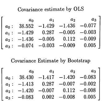
starting from 1911 is used to check how close the bootstrap estimate of the covariance to the OLS estimate is. The regressors include the constant term, the highest speed, the square and the cube of it. The matrix of the estimators are therefore 4 x 4 . The main equation of the regression is: S' = cq + ai x Y + a2 X F2 + 03 X Y^, where Y denotes year, and S denotes the highest speed scored on that year.

The covariance estimates of OLS and bootstrapping are on Table 1.1. Actually, this was a demonstration to reveal that this bootstrap method gives almost the same results given by the OLS method in estimating the covariance. Indeed, the expected values of both of them converge to the same numbers even when the sample size of Monte Carlo simulation is not very high. The minor differences in numbers come from the selection of simulation sample size. Even under this condition the numbers are very close.

The method of bootstrapping again performs well. The reasoning behind this is: we are doing nothing but resampling over the OLS residuals randomly, and calculating the corresponding covariance. Since the Monte Carlo sample

CHAPTER 1. INTRODUCTION

Covariance estimate by OLS

ao «1 «2 «3

«0 : 38.552 -1.429 -1.436 -0.077 «1 : -1.429 0.287 -0.005 -0.003 a2: -1.436 -0.005 0.112 -0.009 «3 : -0.074 -0.003 -0.009 0.005

Covariance Estimate by Bootstrap

do at d3

«0 : 38.430 -1.417 -1.420 -0.083 ai : -1.413 0.287 -0.007 - 0.002 ^2: -1.420 -0.007 0.112 -0.008 (^3: -0.083 0.002 -0.008 0.005

Table 1.1: Covariance estimates by OLS and bootstrap (on the residuals)-Data of IndybOO are used

size is high, the two estimates of covariance are very similar, as can be observed from the table.

1.2.2

Bootstrap by Resampling the Observations

The first procedure of bootstrapping explained above does not allow for het- eroskedasticity since the residuals are randomly scattered. It heavily depends on the OLS residuals being exchangable.

Instead of resampling over the OLS residuals, one can resample over the observations which is more convenient for heteroskedastic regression. In the previous method of bootstrapping, the error terms are calculated and separated from their observations for resampling, but here each observation will keep on holding its error term [14]. The key difference between the two methods is the following : in the first method the residuals are separated from the observations and attached to some other observations, but in the second procedure each observation keeps its own variance of disturbance. Thus, the first method is

supposed to work in cases where the variances of the disturbance terms are similar, that is, in cases close to homoskedasticity whereas since the original observations are kept as they are in the second method, the second method is suitable for the heteroskedastic cases of regression.

The procedure works as follows: the resampling is made over the observa­ tions with replacement. That is, (y j* ,X j), (V^*, X j)) · · · > obtained from (Ti, X i), {Y2,X2)) · · ·) (iT > X r) by T random sampling with replacement. For each resampling, the estimate of ^ is calculated from (T * ,X * ). After ob­ taining the /9*’s for each iteration of Monte Carlo simulation of bootstrapping the covariance matrix is calculated by

Cov/S- = i i ; L , ( A - - W - - W .

This procedure is better displayed in the algorithm, see Figure 1.3.

CHAPTER 1. INTRODUCTION 8

1. Calculate OLS estimate ^

2. Resample the observations, Y ,X with replacement, and get

3. Calculate /3* = for this iteration of bootstrap simu­ lation.

4. If i is less than bootstrap simulation sample size, go to 2. 5. Calculate the bootstrap estimate of ^ from

c o v r = i E L ( A - - / 3 ) ( A · - « ' ·

Figure 1.3: Algorithm explaining the method of bootstrap by resampling the observations

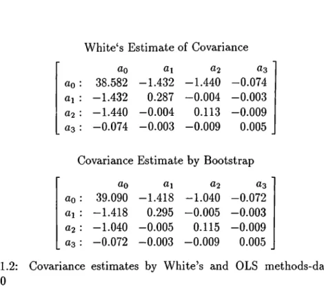
An application of this kind of bootstrapping is made on the data used in the previous case. The estimates by White’s method and this type of bootstrapping for the variance-covariance matrix of ^ are listed in Table 1.2.

CHAPTER 1. INTRODUCTION

White‘ s Estimate of Covariance

ao ai 02 0 3

ao : 38.582 -1.432 -1.440 -0.074 ai : -1.432 0.287 -0.004 -0.003 «2 : -1.440 -0.004 0.113 -0.009 ^3 : -0.074 -0.003 -0.009 0.005

Covariance Estimate by Bootstrap

Co 0,1 02 0 3

ao : 39.090 -1.418 -1.040 -0.072 ai : -1.418 0.295 -0.005 -0.003 a2: -1.040 -0.005 0.115 -0.009 «3 : -0.072 -0.003 -0.009 0.005

Table 1.2: Covariance estimates by White’s and OLS methods-data from IndySOO

estimate for the data are almost the same.

The Tables 1.1, and 1.2 reveal that the bootstrap methods’ ® estimates match White’s and OLS estimates very well. But, we have no opportunity to test how close they are to the actual values of Cov 0, since we did not generate data from some known distribution.

1.2.3

Bootstrap Method Introduced by Wu

Wu (1986) [21] suggested a different method of bootstrapping to find a good estimator in cases of heteroskedasticity. He uses some sort of a weighted boot­ strap in which he assigns weights to the OLS residuals. He uses the following logic of theory:

L e t Y = X/3 + e, e ~ A^(0, H)

®From now on the first method o f bootstrapping, which is done by resampling the O LS residuals, will be denoted by Bootstrap I and the second method, which depends on resam­ pling the observations, will be denoted by Bootstrap II.

CHAPTER 1. INTRODUCTION 10

p = [ X ' X y ^ X ' Y

e = Y - X ^

= Y - X{X'X)-'^X'Y = ( / - X {X ' X ) - ^ X ' ) Y

Let M = I — X{X'X)~^X'. Then it easily follows that

M X = ( / - X { X ' X ) - ^ X ' ) X = X - X { X ’X )- ^ X 'X = X - X i X - y i X ' y ' ^ X ' X = x - x = 0 e = M Y = M { X ^ + e) = M X ^ + Me =0 + Me =Me

Cov e =Cov (Me) =M{Covc)M' ^MDM'

So etlymTt ~ A^(0, cr^),

ep = &t!ymu X Zf, Zt ~ 1V(0,1) gives the weighted errors of bootstrapping.

The rest follows similar to the other methods of bootstrapping, but is slightly different.

CHAPTER 1. INTRODUCTION 11

Y* — + e*. Here in this method, the numbers are obtained from the Zt ~ N {0 , 1) by resampling. That is, instead of resampling the OLS residuals, or the observations, the numbers following standard normal distribution are resampled. The crucial point about these Z ,’s is their means and variances. They must have mean zero, and variance 1, both of which are satisfied with the standard normal distribution. Some inferences about ^ can be made. For example, V агф)=Еф* — — ^)', where is obtained from the above equation and thereby the covariance estimate is obtained.

Now,to calculate the covariance in our context the following formula can be used: Соьф) = (X'X)~^ , where hi is the {г,гУ^ element of the matrix H. See [21].

Note that this is very close to the formula of the true variance, with the key difference that the erf’s are replaced by the weighted OLS residuals. So the problem is reduced to decide whether these weighted residuals can be sub­ stituted for the variances of the disturbance terms, or not. If they can be substituted securely, under which conditions can one do this?

Wu in his paper assumes the conditions under which this substitution can be made. In Lemma 3 at page 1275 he states:

If hij = x'-[X'X)~^Xj for any i,j with <7,- ф <jj, then E e? = (1 — hi)af, and hi = x'-(X'X)~^Xi. A proof is also provided on the same pages. But the more important point for this study is, one of Wu’s global assumptions which re­ quire: max\<i<Tx'i{X'X)~^Xi < c / r , where c is the coefficient of the Fisher’s information matrix. Note that although Wu tries to find an estimator to han­ dle the case of heteroskedasticity he requires a balanced regression which he imposes by his assumption just written. In the expressions above E denotes expected value, and ЬцчГПц are the elements oi H = X{X'X)~^X\ and M = I - X .

The covariance estimate by Wu is calculated depending on the formula he has given, which is

CHAPTER 1. INTRODUCTION 12

C o v 0 ) = (A "A ')-‘ E fe,

The algorithm to explain this Wu’s method of bootstrapping can be ob­ served in Figure 1.4®.

1. Calculate H = X ( X 'X )- i X ’, and M=I-H.

2. Calculate OLS estimate ^ = (X'X)~^X'V. 3. Obtain the OLS residuals e =Y — X^.

4. Assign weights to the residuals and obtain = et/^mu, where mu denotes the entries of M.

5. Calculate i)iyu=diag(e().

6. Calculate Wu’s estimate of covariance from c o v ^wu = { x ’x ) - ^ x ' h w u x { x ' x ) - ' ' .

Figure 1.4: Algorithm explaining Wu’s method of bootstrapping

Chapter 2

Comparison of the Estimators

in Homoskedastic Regression

In this part of the study several methods are taken into consideration and compared in cases of homoskedasticity in different settings. The settings are established to compare the inferiors of the estimators. The high outlier case is included which may affect the performance of the estimators very much. The chapter is divided into three sections. In the first section, performance of OLS, White’s, and three bootstrapping methods are evaluated in case of homoskedasticity where the affect of the value of the common variance of the disturbance terms on the performance of the estimators will be investigated. In the next section, the effect of sample size will be evaluated. Finally, in section three, the performance of the estimators in case of unbalanced regressors will be covered. The unbalancedness will be provided by playing with the last regressor.

CHAPTER 2. HOMOSKEDASTIC REGRESSION 14

2.1

The Effect of the Variance of Disturbance

Terms

This setting is established to handle the case of homoskedasticity where the common variance of the disturbance terms will be changed. The setting is established as follows: first, the regressors are set equal to twenty-one in­ tegers starting from -10 and running till 10. Y is set equal to Xfl -fi e, ct ~ iV(0, iT^), <T = 1,5,10,15,20,25,30.

To make things simpler X is taken to be T x 1, so the covariance matrix turns out to be the variance.

The formulas of true variance. White’s estimate, and OLS estimate of vari­ ance for this setting can be arranged as follows:

{C0V^^)True = E l l

/

{CoV^^)white = E h / ( E h {Cov^)oLS = 0-V X

where is estimated by

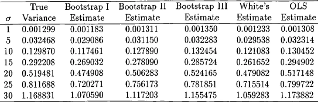
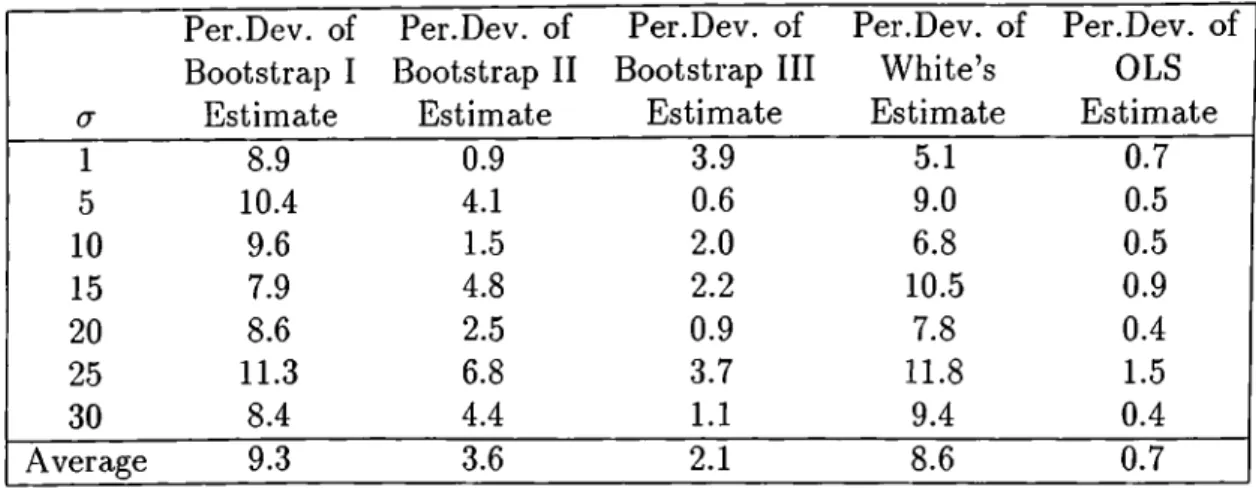
The true variances and the estimates are tabulated in Table 2.1, but it is not very easy to understand the performance of the estimators by simply reading the table, because the true values are changing, as well as the estimators. A second table. Table 2.2, is also given. In this table the percentage deviations of the estimators from the true values are tabulated.

There are two kinds of graphs belonging to these tables. The true values and the estimators are graphed, but this may not give a good picture. So, the percentage deviations of the estimators around the true values are also graphed, and this is what needs to be considered more carefully. The Figure 2.1 ^ displays

CHAPTER 2, HOMOSKEDASTIC REGRESSION 15 cr True Variance Bootstrap I Estimate Bootstrap II Estimate Bootstrap III Estimate White’s Estimate OLS Estimate 1 0.001299 0.001183 0.001311 0.001350 0.001233 0.001308 5 0.032468 0.029086 0.031150 0.032283 0.029538 0.032314 10 0.129870 0.117461 0.127890 0.132454 0.121083 0.130452 15 0.292208 0.269032 0.278090 0.285724 0.261652 0.294902 20 0.519481 0.474908 0.506283 0.524165 0.479082 0.517148 25 0.811688 0.720271 0.756173 0.781851 0.715514 0.799722 30 1.168831 1.070590 1.117203 1.155475 1.059283 1.173882

Table 2.1: Performance of the estimators, homoskedasticity, changing variances

the plot of the estimators along the true values, and the percentage deviations of them around the true values.

The tables and the graphs reveal that the estimators are all good in this setting. The average percentage deviations are all less than ten percent. OLS gives the best estimator. Anyway, this is what is stated by the theory. It almost hits the true values. Although it is not as good as OLS estimator, the Bootstrap III estimator is also very good. The Bootstrap II estimator follows these two, and its average percentage deviation is small. Although White’s estimator is especially designed for heteroskedastic regression it performs better than the Bootstrap I estimator.

The graphs reveal that as the common variance of the disturbance terms increase, Bootstrap II, and White’s estimates have a tendancy to become worse.

2.2

The Effect of Sample Size

The same setting can be used to understand the effect of sample size on the performance of the estimators. Everything is the same as what they were in

CHAPTER 2. HOMOSKEDASTIC REGRESSION 16 a Per.Dev. of Bootstrap I Estimate Per.Dev. of Bootstrap II Estimate Per.Dev. of Bootstrap III Estimate Per.Dev. of White’s Estimate Per. Dev. of OLS Estimate 1 8.9 0.9 3.9 5.1 0.7 5 10.4 4.1 0.6 9.0 0.5 10 9.6 1.5 2.0 6.8 0.5 15 7.9 4.8 2.2 10.5 0.9 20 8.6 2.5 0.9 7.8 0.4 25 11.3 6.8 3.7 11.8 1.5 30 8.4 4.4 1.1 9.4 0.4 Average 9.3 3.6 2.1 8.6 0.7

Table 2.2: Percentage Deviations of the estimators, homoskedasticity, changing variances

the previous setting, but this time instead of changing the common variance of the disturbance terms the sample size, T will be changed. The setting can be summarized as follows:

X = -[ T /

2

2

2

2

Y = X/3 + e, 13 = 1, Var e = 25, t=10,15,20,30,40,50,60.

Again the true variance and the estimators are given first in Table 2.3, and Figure 2.2, displays the percentage deviations of the estimators.

In the previous section while the variance of the disturbance terms were being increcLsed the sample size of the observations was fixed to 21. It is interesting to see here that as the sample size gets higher. Bootstrap I, and W hite’s estimators are having a significant trend to come closer to the true values. In this setting Bootstrap II, Bootstrap III, and, needless to say, OLS estimators are performing very well. Again all the estimators are good. But the best is the OLS method, followed by Wu’s method of bootstrapping. Looking

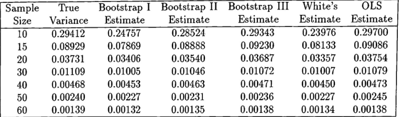
CHAPTER 2. HOMOSKEDASTIC REGRESSION 17 Sample Size True Variance Bootstrap I Estimate Bootstrap II Estimate Bootstrap III Estimate W hite’s Estimate OLS Estimate 10 0.29412 0.24757 0.28524 0.29343 0.23976 0.29700 15 0.08929 0.07869 0.08888 0.09230 0.08133 0.09086 20 0.03731 0.03406 0.03540 0.03687 0.03357 0.03754 30 0.01109 0.01005 0.01046 0.01072 0.01007 0.01079 40 0.00468 0.00453 0.00463 0.00471 0.00450 0.00473 50 0.00240 0.00227 0.00231 0.00236 0.00227 0.00245 60 0.00139 0.00132 0.00135 0.00138 0.00134 0.00138

Table 2.3: Performance of the estimators, homoskedasticity, changing sample size Sample Size Per. Dev. of Bootstrap I Estimate Per.Dev. of Bootstrap II Estimate Per.Dev. of Bootstrap III Estimate Per.Dev. of White’s Estimate Per.Dev. of OLS Estimate 10 15.8 3.0 0.2 18.5 1.0 15 11.9 0.5 3.4 8.9 1.8 20 8.7 5.1 1.2 10.0 0.6 30 9.4 5.7 3.3 9.2 2.7 40 3.2 1.1 0.6 3.8 1.1 50 5.4 3.7 1.7 5.4 2.1 60 5.0 2.9 0.7 3.6 0.7 Average 8.5 3.1 1.6 8.5 1.4

Table 2.4: Percentage Deviations of the estimators, homoskedasticity, changing sample size

CHAPTER 2. HOMOSKEDASTIC REGRESSION 18

at the Bootstrap III estimator and the true values from Table 2.3 one can observe that the estimator is sometimes less and sometimes greater than the true value. So, the simulation results say that there is not a bias on some direction. The situation is the same for the OLS estimator.

2.3

The Effect of Outliers

This final section of the chapter is devoted to the effect of changing outliers on the performance of the estimators. The last regressor is changed to establish this new setting. The sample size is fixed to 21 again. The setting is designed as follows :

X = -10,-9, . . .,9,X[21]. Y = = 1, Var e = 25, the outliers are 20,30,40,50,60, and 70.

This kind of a setting leads to some scattered regressors which are the leverage points and, the outliers of the regression analyses. The high regressors may make the estimators perform even worse.

The performance of the estimators is tabulated in Table 2.5, and displayed in Figure 2.3.

These results reveal that the performance stability of the estimators is de­ stroyed, and the performance heavily depends on how much deviant the highest regressor is.

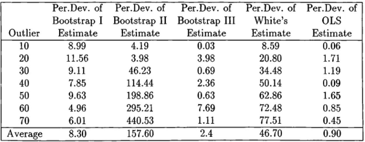
To give a better insight the percentage deviations of the estimators from the true values are also tabulated and graphed in Table 2.6, and Figure 2.3.

The presence of the outliers offered a good opportunity to differentiate be­ tween the performance of the estimators. Bootstrap I estimator is not affected from the changes in variance of the disturbance terms, the sample size, and the outliers. Its percentage deviation is around 8 percent. On the other hand.

CHAPTER 2. HOMOSKEDASTIC REGRESSION 19 Outlier True Variance Bootstrap I Estimate Bootstrap II Estimate Bootstrap III Estimate White’s Estimate OLS Estimate 10 0.03247 0.02955 0.03111 0.03248 0.02968 0.03245 20 0.02336 0.02066 0.02429 0.02243 0.01850 0.02296 30 0.01592 0.01447 0.02328 0.01603 0.01043 0.01573 40 0.01101 0.01015 0.02362 0.01127 0.00549 0.01100 50 0.00789 0.00713 0.02358 0.00794 0.00293 0.00776 60 0.00585 0.00556 0.02312 0.00540 0.00161 0.00590 70 0.00449 0.00422 0.02427 0.00454 0.00101 0.00447

Table 2.5: Performance of the estimators, homoskedasticity, outliers

Outlier Per.Dev. of Bootstrap I Estimate Per.Dev. of Bootstrap II Estimate Per.Dev. of Bootstrap III Estimate Per.Dev. of White’s Estimate Per.Dev. of OLS Estimate 10 8.99 4.19 0.03 8.59 0.06 20 11.56 3.98 3.98 20.80 1.71 30 9.11 46.23 0.69 34.48 1.19 40 7.85 114.44 2.36 50.14 0.09 50 9.63 198.86 0.63 62.86 1.65 60 4.96 295.21 7.69 72.48 0.85 70 6.01 440.53 1.11 77.51 0.45 Average 8.30 157.60 2.4 46.70 0.90

CHAPTER 2. HOMOSKEDASTIC REGRESSION 20

although Bootstrap II estimators were very well when there were no outliers, this time they failed very badly, and Bootstrap II, and White’s estimators have a significant trend to deviate away from the true values as the regression be­ comes more unbalanced. Wu’s estimator is not affected from the presence of the outliers as well as the OLS estimator. White’s method is also affected from the outliers, and it consistently moves away from the true value as the outlier deviates more.

So the two good estimators which were able to achieve well in all cases of homoskedasticity are by Wu and OLS.

The performance of the estimators in homoskedastic regression is summa­ rized in a table in the last pages of the thesis in conclusion.

CHAPTER 2. HOMOSKEDASTIC REGRESSION

Bootstrap I

Bootstrap II

Bootstrap III

White

O L S

21

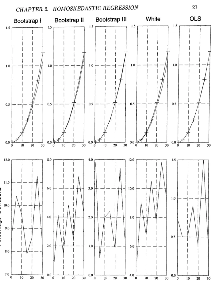
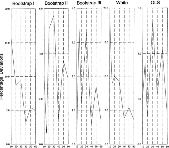
Figure 2.1: Performance of the estimators, homoskedasticity, changing vari­ ances

CHAPTER 2. HOMOSKEDASTIC REGRESSION 22

Bootstrap I

Bootstrap II

Bootstrap III

White

O L S

Figure 2.2: Performance of the estimators, homoskedasticity, changing sample size

CHAPTER 2. HOMOSKEDASTIC REGRESSION

Bootstrap I

Bootstrap II

Bootstrap III

White

23

O L S

Chapter 3

Comparison of the Estimators

in Heteroskedastic Regression

In this part of the thesis the estimators will be tested under heteroskedastic regression. This chapter is an important part of the thesis, because as it was stated before OLS is a perfect estimator for the homoskedastic regression whatever the sample size or the outlier is. But finding a reliable estimator for the heteroskedastic regression is problematic. One purpose of including the bootstrap methods in the thesis is to find a good estimator with this method at least for some cases. The chapter will be comprising five sections. In the first three sections the performance of the estimators will be evaluated under different kinds of heteroskedasticity. Then in the last two sections the effects of increasing the sample size and outliers will be examined.

3.1

Simple Case of Heteroskedasticity

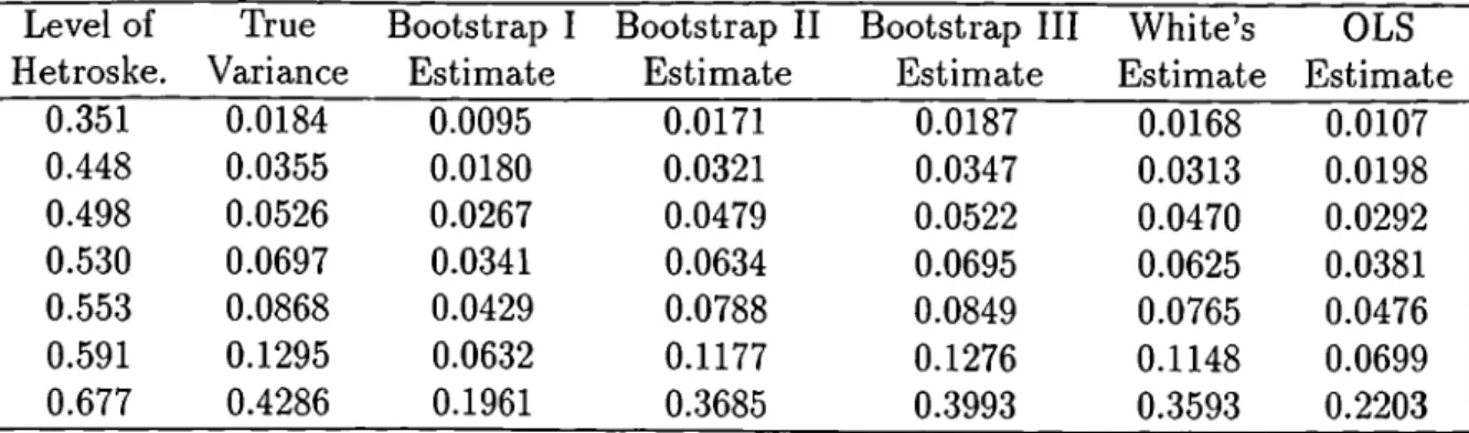
In this first setting of the chapter the regressors are selected just how they were selected before, that is, the consequent integers which sum up to zero approximately are selected as the regressors. The sample size of observations,T is set equal to 21, so X =-10,-9,.. .,9,10. The variances of the disturbance terms

CHAPTER 3. HETEROSKEDASTIC REGRESSION 25 Level of Hetroske. True Variance Bootstrap I Estimate Bootstrap II Estimate Bootstrap III Estimate White’s Estimate OLS Estimate 0.351 0.0184 0.0095 0.0171 0.0187 0.0168 0.0107 0.448 0.0355 0.0180 0.0321 0.0347 0.0313 0.0198 0.498 0.0526 0.0267 0.0479 0.0522 0.0470 0.0292 0.530 0.0697 0.0341 0.0634 0.0695 0.0625 0.0381 0.553 0.0868 0.0429 0.0788 0.0849 0.0765 0.0476 0.591 0.1295 0.0632 0.1177 0.1276 0.1148 0.0699 0.677 0.4286 0.1961 0.3685 0.3993 0.3593 0.2203

Table 3.1: Performance of the estimators, heteroskedasticity, simple case

will be set equal to 1+bJf^. Level of heteroskedasticity will be adjusted by playing with b.

In order to evaluate the results, some sort of a measure for heteroskedas­ ticity has to be used. The value, ( F l t i af) can be used for this purpose, but this value decreases as the regression becomes more het- eroskedastic, and vice versa. Instead (-2 x log) of this value will be used to determine how much heteroskedastic the regression is.^

The results corresponding to this case are listed in Table 3.1. These results are also graphed in Figure 3.1.

The table is repeated with the percentage deviations of the estimators. The corresponding table is Table 3.2.

Looking at the graphs perhaps the first comment to make is the trend of all estimators to become worse as the level of heteroskedasticity increases. The best estimator of the last chapter, the OLS estimate, is too bad this time, which together shows how much sensitive the OLS estimator to the assumption of homoskedasticity is. The Bootstrap I estimator is also very bad, and cannot

^This value will be used to determine the level of heteroskedasticity in some different parts o f the thesis that will come later

CHAPTER 3. HETEROSKEDASTIC REGRESSION 26

Perc. Dev. of Perc. Dev. of Perc. Dev. of Perc. Dev. of Perc. Dev. of Level of Bootstrap I Bootstrap II Bootstrap III White’s OLS

Hetroske. Estimate Estimate Estimate Estimate Estimate

0.351 48.4 7.1 1.6 8.7 41.8 0.448 49.3 9.6 2.3 11.8 44.2 0.498 49.2 8.9 0.8 10.6 44.5 0.530 51.1 9.0 0.3 10.3 45.3 0.553 50.6 9.2 2.2 11.9 45.2 0.591 51.2 9.1 1.5 11.4 46.0 0.677 54.2 14.0 6.8 16.2 48.6 Average 50.6 9.6 2.2 11.6 45.1

Table 3.2: Percentage deviations of the estimators, heteroskedasticity, simple case

be used to estimate the covariance at all.

It was already said in the introduction that although White’s method was originally designed to handle the case of heteroskedasticity, it was shown to be biased. Its percentage deviation is around 11 percent. Bootstrap II is similar to W hite’s method, and is a bit better than that.

The best estimator of the section is Bootstrap III, Wu’s method of boot­ strapping. It keeps its performance as the setting is changed from homoskedas- ticity to heteroskedasticity. The reason for this is sourced from the weights it distributes to the OLS residuals, as was explained in introduction.

3.2

Complicated Case of Heteroskedasticity

This section is very similar to the previous one. The unique difference comes from the variances of the disturbance terms. Instead of setting the variances of the disturbance terms equal to l+ b *A ’^^, this time the variances are set equal to (1-1-6 + X - l - c * X'^y. This update on variances bring heteroskedasticity from both the 6 * X , and the c * X'^ terms. The regressors are not changed.

CHAPTER 3. HETEROSKEDASTIC REGRESSION 27 Level of Hetroske. True Variance Bootstrap I Estimate Bootstrap II Estimate Bootstrap III Estimate White’s Estimate OLS Estimate 1.641 2.5918 1.0871 2.3341 2.6439 2.3563 1.2115 1.653 1.8406 0.7471 1.5883 1.7863 1.5925 0.8219 1.667 6.9313 2.9293 6.3696 7.1311 6.3548 3.2530 1.697 1.2229 0.5022 1.0635 1.1844 1.0575 0.5574 1.713 15.3588 6.4912 13.9495 15.7718 14.0544 7.1939 1.859 0.7387 0.3155 0.6691 0.7463 0.6658 0.3489 2.224 0.3879 0.1622 0.3348 0.3706 0.3317 0.1814

Table 3.3; Performance of the estimators, heteroskedasticity, complicated case

X = -1 0 ,-9 ,.. .,9,10. Y — + e,0 = 1 as usual.

The results for this setting are given in Tables 3.3, and 3.4.

The percentage deviations are tabulated in Table 3.4 and are displayed in Figure 3.2.

This setting reveals two important features of the estimators. First each estimator’s performance becomes poorer. And secondly, the trend of the esti­ mators to deviate more as the level of heteroskedasticity, has lost its significance this time.

Wu’s method of bootstrapping still performs very well.

3,3

The Case of Random Heteroskedasticity

The type of heteroskedasticity of the regression can be changed by adding ran­ dom terms to the variances of the disturbance terms. This change in variance constitutes the third case of heteroskedaaticity. The setting will not be changed again. The purpose of keeping the setting the same is to establish the same

CHAPTER 3. HETEROSKEDASTIC REGRESSION 28 Level of Hetroske. Perc. Dev. of Bootstrap I Estimate Perc. Dev. of Bootstrap II Estimate Perc. Dev. of Bootstrap III Estimate Perc. Dev. of White’s Estimate Perc. Dev. of OLS Estimate 1.641 58.0 9.9 2.0 9.1 53.3 1.653 59.4 13.7 2.9 13.5 34.2 1.667 42.3 8.1 2.9 8.3 53.1 1.697 58.9 13.0 3.1 13.5 54.4 1.713 57.7 9.2 2.7 8.5 46.8 1.859 57.3 9.4 1.0 9.9 52.8 2.224 58.2 13.7 4.5 14.5 53.2 Average 56.0 11.0 2.7 11.0 49.7

Table 3.4; Percentage deviations of the estimators, heteroskedasticity, compli­ cated case

ground for the comparisons. The consequent integers around zero are used as the regressors with sample size 21, Y — X ^ + e. And the variances of the distur­ bance terms are = 1 + bX^ + v^, 6 = 1, i/ ~ N[Q, a^), a — 1 ,2 ,3 ,4 ,5 ,6 ,7 ,8 . The effect of changing b is similar to changing it in the simple case of het­ eroskedasticity. Here the main emphasis is on observing the effects of changes in a which increases the randomness and the level of heteroskedasticity. This new setting can be summarized as follows:

X = -1 0 ,-9 ,.. .,9,10, Y = X 0 -l-t, ^ ^ 1 ,

N{<d,a^^),a} = \ + h X ‘} + v l b = l,u ^ N{Q,a^), a = 1 ,2 ,3 ,4 ,5 ,6 ,7 ,8 .

The corresponding table and graphs for this setting are Table 3.5, and Figure 3.3.

Again the percentage deviations are given in Table 3.6.

OLS and Bootstrap I have an increasing deviation as the level of het­ eroskedasticity gets higher, but the other estimators do not have a regular pattern of trend in this random heteroskedasticity. Wu’s method of bootstrap­ ping performs perfectly again. Bootstrap I, and OLS estimators are very bad.

CHAPTER 3. HETEROSKEDASTIC REGRESSION 29 Level of Hetroske. True Variance Bootstrap 1 Estimate Bootstrap 11 Estimate Bootstrap III Estimate White’s Estimate OLS Estimate 0.339 0.2361 0.1398 0.2158 0.2304 0.2083 0.1536 0.346 0.2190 0.1275 0.2038 0.2167 0.1957 0.1399 0.361 0.2043 0.1135 0.1874 0.2010 0.1815 0.1258 0.385 0.1932 0.1035 0.1712 0.1854 0.1673 0.1122 0.433 0.1836 0.0941 0.1670 0.1822 0.1641 0.1057 0.449 0.1735 0.0858 0.1575 0.1733 0.1559 0.0953 0.483 0.1773 0.0883 0.1567 0.1712 0.1543 0.0975

Table 3.5; Performance of the estimators, random heteroskedasticity

Level of Hetroske. Perc. Dev. of Bootstrap I Estimate Perc. Dev. of Bootstrap II Estimate Perc. Dev. of Bootstrap III Estimate Perc. Dev. of White’s Estimate Perc. Dev. of OLS Estimate 0.339 40.8 8.6 2.4 11.8 34.9 0.346 41.8 6.9 1.1 10.6 36.1 0.361 44.4 8.3 1.6 11.2 38.4 0.385 46.4 11.4 4.0 13.4 41.9 0.433 48.7 9.0 0.8 10.6 42.4 0.449 50.5 9.2 0.1 11.1 43.8 Average 45.4 8.9 1.7 11.5 39.3

CHAPTER 3. HETEROSKEDASTIC REGRESSION 30 Sample Size True Variance Bootstrap I Estimate Bootstrap II Estimate Bootstrap III Estimate White’s Estimate OLS Estimate 10 0.1963 0.0841 0.1566 0.1772 0.1405 0.1026 20 0.0921 0.0440 0.0795 0.0871 0.0779 0.0488 30 0.0606 0.0317 0.0580 0.0617 0.0573 0.0336 40 0.0453 0.0230 0.0413 0.0435 0.0412 0.0240 50 0.0361 0.0198 0.0358 0.0373 0.0358 0.0207 60 0.0301 0.0161 0.0292 0.0302 0.0292 0.0167 70 0.0258 0.0137 0.0249 0.0257 0.0249 0.0141

Table 3.7: Performance of the estimators, heteroskedasticity, simple case, changing sample size

Bootstrap II, and White’s estimators are about ten percent different than the true values on the average.

3.4

Heteroskedasticity with Changing Sam­

ple Sizes

This setting turns from random heteroskedasticity to simple heteroskedasticity. So X = -[T /2 ],-[T /2 ]+ l,.. .,[T/2]-l,[T/2], Y=X/9 + e, The sample size will be 10 at the beginning, and then it will rim to 60 with increments of 10. The figures obtained out of this setting are listed in Table 3.7 and the graph of them is arranged in Figure 3.4.

The percentage deviations are tabulated in Table 3.8, and the plot of these deviations are on Figure 3.4.

The type of heteroskedasticity used here is the simple one of the first section of this chapter. The main objective of this section is to assess the effect of sample size on the estimators. Table 3.8, and Figure 3.4 reveal that all the

CHAPTER 3. HETEROSKEDASTIC REGRESSION 31 Sample Size Perc. Dev. of Bootstrap I Estimate Perc. Dev. of Bootstrap II Estimate Perc. Dev. of Bootstrap III Estimate Perc. Dev. of White’s Estimate Perc. Dev. of OLS Estimate 10 57.2 20.2 9.7 28.4 47.7 20 52.2 13.7 5.4 15.4 47.0 30 47.7 4.3 1.8 5.4 44.5 40 49.2 8.8 4.0 9.1 47.0 50 45.1 0.8 3.3 0.8 42.7 60 46.5 3.0 0.3 3.0 44.5 70 46.9 3.5 0.4 3.5 45.3 Average 49.3 7.8 3.6 9.4 45.5

Table 3.8: Percentage deviations of the estimators, heteroskedasticity, simple case, changing sample size

estimators are getting better as the sample size of the observations, T is higher, significantly. Again, Bootstrap I, and OLS estimators are so bad that they cannot be used for the purpose of estimation. The bootstrap method suggested by Wu is the best.

3.5

Heteroskedastic Regression with Outliers

In this last setting of the last chapter for testing the estimators in case of het­ eroskedasticity nothing is changed but the regressors are now including outliers. Despite of being a unique change in the setting, this leads to changes in the phenomena much. Since the variances of the disturbance terms were set equal to 1 -f the variances change very much. On the other hand, high regres­ sors are made possible which results in outliers and leverage points. Again the setting can be summarized as follows:

X = - 1 0 , - 9 , . . . , 9 , X [ T ] , r = 21,

X[T] = 10,20,30,40,50,60,70.Y = X + e,

CHAPTER 3. HETEROSKEDASTIC REGRESSION 32 Outlier True Variance Bootstrap I Estimate Bootstrap II Estimate Bootstrap III Estimate White’s Estimate OLS Estimate 10 0.0868 0.0438 0.0793 0.0870 0.0784 0.0483 20 0.1762 0.0395 0.1159 0.1414 0.1009 0.0432 30 0.3457 0.0288 0.1590 0.1569 0.0777 0.0313 40 0.5051 0.0239 0.2449 0.2841 0.0623 0.0259 50 0.6263 0.0187 0.3003 0.1634 0.0399 0.0201 60 0.7133 0.0143 0.3232 0.3230 0.0242 0.0151 70 0.7754 0.0107 0.3300 0.1021 0.0143 0.0115

Table 3.9: Performance of the estimators, heteroskedasticity, simple case, out­ liers

The performance of the estimators are tabulated in Table 3.9, the percent­ age deviations are also tabulated in Table 3.10. The corresponding graphs are plotted in Figure 3.5.

The Bootstrap II is very sensitive to the outliers, because it is very impor­ tant to have a balanced regression for Bootstrap II. It has to select the outlying regressor ((1 /T ) x Monte Carlo simulation sample size) times. Whether it takes the outlying regressor more or less than this number makes much differ­ ence to the performance of Bootstrap II estimates.

In this final section of the chapter the emphasis is on understanding the effect of outliers on the performance of the estimators. Figure 3.5 shows very explicitly that as the outlier is increased, the gap between the true values and the estimates become larger. The graphs at the bottom also shows this same thing. There is a very sharp trend of increase in the percentage deviations of the estimators as the outlier becomes larger. Table 3.9 shows that all the esti­ mators are less than the true variance. When the outlier is 70, the percentage deviations of three estimators, all but Bootstrap II and White’s estimators, are more than 90 percent.

CHAPTER 3. HETEROSKEDASTIC REGRESSION 33

Perc. Dev. of Perc. Dev. of Perc. Dev. of Perc. Dev. of Perc. Dev. of Outlier Bootstrap I Bootstrap II Bootstrap III White’s OLS

Estimate Estimate Estimate Estimate Estimate

10 49.5 8.6 0.2 9.7 44.2 20 77.8 34.2 19.7 42.7 75.5 30 91.7 46.0 54.6 77.5 90.9 40 95.3 51.5 43.8 87.7 94.9 50 97.0 52.1 73.9 93.6 96.8 60 98.0 54.7 77.3 96.7 97.9 70 98.6 57.4 86.8 98.2 98.5 Average 86.8 43.5 50.9 72.3 85.5

Table 3.10: Percentage deviations of the estimators, heteroskedasticity, simple case, outliers

of bootstrapping, fails in this final setting. So there is no unique estimator which is good in all cases. Actually, there is no good estimator for this last case.

CHAPTER 3. HETEROSKEDASTIC REGRESSION

Bootstrap I

Bootstrap II

Bootstrap III

White

O L S

34

CHAPTER 3. HETEROSKEDASTIC REGRESSION 35

Bootstrap I

Bootstrap II

Bootstrap

White

60.0

50.0

30.0

4 0 .0---i---,---r

CHAPTER 3. HETEROSKEDASTIC REGRESSION

Bootstrap I

Bootstrap II

Bootstrap III

White

0.25 0.22 — z b 0.20 — 0.18 — 0.16 — 0.14 0.20 0.15 — 0.10 — 0.05

CHAPTER 3. HETEROSKEDASTIC REGRESSION

Bootstrap I

Bootstrap II

Bootstrap III

White

0.20

I

I

I

i i

1

il I

- I j r ' r -

Figure 3.4: Performance of the estimators, heteroskedasticity, simple case, changing sample sizes

CHAPTER 3. HETEROSKEDASTIC REGRESSION

Bootstrap I

Bootstrap II

Bootstrap III

White

_{O LS}

38

Chapter 4

Conclusion

The results of the Monte Carlo simulations are in parallel to the theory all the time. But the question of finding a good estimator for both homoskedastic and heteroskedastic settings is still open.OLS and bootstrap III methods perform very well in settings of homoskedasticity and bootstrap II method performs the best in cases of heteroskedasticity, which together say that Bootstrap III is the best in the overall picture, but it is not good in cases of unbalanced regressors.

A table is prepared to display the performance of the estimators in the settings covered so far, see Figure 4.1.

So far, we already know that whatever the case is OLS estimates perfectly when the regression is homoskedastic, regardless of the regression being bal­ anced or not. And, Wu’s method works perfectly, in case of homoskedasticity and heteroskedasticity in the absence of the outliers. But is not a remedy of finding a reliable estimator, for heteroskedastic regression with outliers, be­ cause it is not possible to satisfy its assumptions when the regression is unbal­ anced. So, there is no estimator available for this case. And, this remains as a good area of research. The bias correction methods may be used to settle this problem.

CHAPTER 4. CONCLUSION 40

Estimate Bootstrap I Bootstrap II Bootstrap III White OLS (Average % oO (Average % oO (Average % oO (Average % of) (Average % of) Setting (Deviation) (Deviation) (Deviation) (Deviation) (Deviation) Homoskedasticity Good _{Very Good Very Good} Good _{Very Good}

Changing Variances _{(9.3) (3.6) (2.1) (8.6) (0.7)}

Homoskedasticity Good _{Very Good Very Good} Good _{Very Good} Changing Sample Size _{(8.5) (3.1) (1.6) (8.5) (1.4)} Homoskedasticity Good Very Bad _{Very Good} Bad _{Very Good}

Outliers _{(8.3) (157.6) (2.4) (46.7) (0.9)}

Heteroskedasticity Bad Good Very Good Good Bad

Simple Case _{(50.6) (9.6)} (2.2) _{(11-6) (45.1)}

Heteroskedasticity Very Bad Good _{Very Good} Good Bad Complicated Case _{(56.0) (11.0) (2.7) (11.0) (49.7)}

Heteroskedasticity Bad Good _{Very Good} Good Bad

Random _{(45.4) (8.9) (1.7) (11.5) (39.6)}

Heteroskedasticity Bad Good _{Very Good} Good Bad

Changing Sample Size _{(49.3) (7.8) (3.6) (9.4) (45.5)} Heteroskedasticity Very Bad Bad Very Bad Very Bad Very Bad

Outliers _{(86.8) (43.5) (50.9) (72.3)} (85.5)

Bibliography

[1] A., Chesher The Information Matrix Test - Simplified Calculation via a Score Test Interpretation Economics Letters, 13, 45-48, 1983.

[2] A., Chesher, and I., Jewitt The Bias of a Heteroskedasticity-Consistent Covariance Matrix Estimator Econometrica, 55, 1217-1222, 1987.

[3] A., Chesher, and R., Spady Asymptotic Expansions of the Information Matrix Test Statistic Econometrica, 59, 787-815, 1991.

[4] A.C., Davison, D.V., Hinkley, and E., Schechetman Efficient Bootstrap Simulation Biometrica, 73, 555-566, 1986.

[5] T., Diciccio, and J., Romano A Review of Bootstrap Confidence Intervals Journal of Royal Statistical Society, 50, 338-354, 1988.

[6] B., Efron Bootstrap Methods: Another look at jacknife The Annals of Statistics, 7, 1-26, 1979.

[7] B., Efron The Jackknife, the Bootstrap and other Resampling Plans CBMS-NSF Regional Conference Series in Applied Mathematics, Mono­ graph 38, 1982.

[8] F., Eicker Asymptotic Normality and the Consistency of the Least Squares Estimates for the Families of Linear Regressions Annals of Mathematical Statistics, 34, 447-456, 1963.

[9] D.A., Freedman, and S.C., Peters Bootstrapping a Regression Equation: Some Empirical Results Journal of the American Statistical Association, 79, 97-106, 1984.

BIBLIOGRAPHY 42

[10] P., Hall The Bootstrap and Edgeworth Expansions New York, Springer- Verlag, 1992.

[11] J.L., Horowitz Bootstrap based Critical Values for the Infirmation Matrix Test Journal of Econometrics, 61, 395-411, 1994.

[12] D.,V., Hinkley Bootstrap Methods Journal of Royal Statistical Society, 50, 321-337, 1988.

[13] D.V., Hinkley, and S., Shi Importance Sampling and the Nested Bootstrap Biometrica, 76, 435-446, 1989.

[14] J., Jeong, and G.S., Maddala A Perspective on Application of Bootstrap Methods in Econometrics Handbook of Statistics, 11, 1992.

[15] T., Lancaster The Covariance Matrix of the Information Matrix Test Econometrica, 52, 1051-1054, 1992.

[16] R., Liu Bootstrap Procedures under some non i.i.d. Models Annals of Statistics, 16, 1696-1708, 1988.

[17] J.G., Mackinnon, and H. White Some Heteroskedastic Consistent Co- variance Estimators with Improved Finite Sample Properties Journal of Econometrics, 29, 305-325, 1985.

[18] G.S., Maddala Econometrics Mcgraw-Hill, New York, 1977.

[19] W ., Navidi Edgeworth Expansion for Bootstrapping Regression Models The Annals of Statistics, 17, 1472-1478, 1989.

[20] H., White A Heteroskedasticity-Consistent Covariance Matrix Estimator and a Direst Test for Heteroskedasticity Econometrica, 48, 817-838, 1980. [21] C.F.J., Wu Jackknife, Bootstrap, and Other Resampling Methods in Re­