FELDSTEIN-HORIOKA PUZZLE IN TURKEY
TÜRKİYE’DE FELDSTEIN-HORIOKA SORUNSALI Gülten DURSUN(1), Tezcan ABASIZ(2)
(1)Kocaeli Üniversitesi, İİBF, İktisat Bölümü
(2)Bülent Ecevit Üniversitesi, İİBF, İktisat Bölümü
(1)[email protected], (2)[email protected]
ABSTRACT: In this study, Feldstein-Horioka hypothesis on saving-investment relationship was tested for the period 1968-2008 in Turkey using Hansen-Seo, Gregory-Hansen and Hatemi-J models. First of all, when Feldstein-Horioka hypothesis was researched by Hansen-Seo method, the variables did not exhibit a nonlinear structure. Then, with Gregory-Hansen and Hatemi-J models, it was found that the saving-retention coefficient got a value close to 1 and 0.426 respectively. It was understood that the Feldstein-Horioka puzzle continued. The results obtained show that in testing Feldstein-Horioka hypothesis, instead of a fixed parameter assumption, applying test techniques that take endogenous structural breaks into consideration would give more reliable results.
Keywords: Feldstein-Horioka Puzzle; Threshold Cointegration Model; Gregory Hansen; Hatemi-J Model
JEL Classification: E22; F21; C32
ÖZET: Bu çalışmada Hansen-Seo, Gregory-Hansen ve Hatemi-J modelleri kullanılarak Türkiye’de Feldstein-Horioka hipotezi 1968-2008 dönemi için test edilmiştir. Öncelikle Feldstein-Horioka hipotezi Hansen-Seo yöntemiyle araştırılmış, değişkenlerin uzun dönemde doğrusal olmayan bir yapı izlemediği bulgusuna ulaşılmıştır. Daha sonra Gregory-Hansen ve Hatemi-J modelleri çerçevesinde tasarruf tutma katsayısı sırasıyla 1’e yakın ve 0.426 olarak elde edilmiş Feldstein-Horioka sorunsalının devam ettiği gözlenmiştir. Elde edilen sonuçlar F-H hipotezinin test edilmesinde sabit bir parametre varsayımı yerine endojen yapısal kırılmaları dikkate alan test tekniklerinin uygulanmasının daha güvenilir sonuçlar verebileceğini göstermiştir
Anahtar Kelimeler: Feldstein-Horioka Sorunsalı; Eşik Eşbütünleşme; Gregory-Hansen; Hatemi-J Modeli
1. Introduction
The international financial integration degree which is defined in connection with the financial markets has shown a significant increase both in developed and developing countries since the 1980s as result of technological developments, financial liberalization and the growth in volume of world trade. When large current account deficits of many countries appeared, particularly the relationship between domestic savings and investments became the focus issue of the discussions in international macroeconomy. When it is accepted that capital movements have a positive effect on development, it becomes important to measure this mobility (Andrade, 2008:22).
The traditional approach in testing the capital mobility hypothesis is the Feldstein-Horioka (1980; hereafter FH) pioneer study. The question “How mobile is the world
capital supply in international sense?” has been the question tried to be answered by FH. According to FH approach, in a world where international capital flows are free, an increase in domestic savings should not create a change in domestic investments. Feldstein and Horioka (1980), Feldstein (1983), and Feldstein and Bacchetta (1989) interpreted the positive correlation coefficient among the variables as a proof of the low degree of long term international capital mobility. High correlation coefficient means that investments are financed by domestic savings. On the contrary, low coefficient shows that investments are financed by international savings. This means that the capital moves from less productive countries to more productive ones (Hogendorn, 1998:142). When domestic saving and investment rates are equal, current account balance will be close to zero. Feldstein and Horioka carried out an emprical study in order to measure the degree of capital mobility over the period 1960-1974 for sixteen OECD countries. In the findings they obtained, the saving-retention coefficient is a value close to 1. Only 5-15% of the national savings are financed by foreign investments. They interpreted this result as a proof of the low capital mobility during the concerned period, in contrast to with the idea that international capital flows integrate quickly. This result was taken by surprise especially in finance area. Because the capital mobility among the OECD countries was very high during the concerned period and there were important transformations concerning the liberalization of the capital markets. Some studies that were carried out also supported the results of FH (Feldstein, 1983; Dooley et al., 1987; Tesar, 1991; Narayan, 2005). However, as they did not correspond to reality, the findings obtained were called as “FH puzzle” in literature.
In this study we aim to test the FH hypothesis in Turkey during the period 1968-2008 with the help of two-regime threshold cointegration, Gregory-Hansen (1996) and Hatemi-J (2008) models. The first model is important as it takes into the long term nonlinear relationship between savings and investment. The second and third models allow us to test whether the FH puzzle continues to be a problem in single and double breaks. Thus, each three model used in the study will give the opportunity to compare whether the findings about FH hypothesis are consistent or not. We also show whether the emprical findings can be interpreted as a reliable indicator for Turkey especially with respect to capital mobility degree.
The rest of the article is as follows. In the second section, we explain the theoretical explanation of the threshold cointegration test developed by Hansen-Seo (2002). That the explanation power of traditional unit root tests in the unit root analyses of the series with a threshold structure is low made it essential to choose the suitable one of the threshold autoregression (TAR) unit root tests out of the tests applied. In the third section, we introduce briefly the single-structural break cointegration test developed by Gregory-Hansen (1996) and the two-structural break cointegration test developed by Hatemi-J (2008). In section four we introduce the related data set. In section five, we give the empirical test results. Finally, section six concludes with the evaluation of the findings.
2. Literature Review
The FH puzzle, which has found wide coverage in literature, has been the subject of important discussions aiming to explain the international capital mobility and puzzle. The solution of FH puzzle is important as it depends on the degree of saving-investment (hereafter S-I) correlation of economic policies which support the
domestic savings (Telatar et al. 2007: 524). If there is strong correlation between two variables, the economic policies supporting the domestic savings will increase the domestic investments. Otherwise, such kind of policies will not have any effect on the internal investments due to the increase in international capital flows.
The studies aiming at solving the FH puzzle can be classified in two ways: the theoretical inference of the FH coefficient and economic modelling problems (Telatar et al. 2007). In the discussions regarding theoretical inference, unlike Feldstein and Horioka, some studies interpreted the high FH coefficient as an evidence of high international capital mobility. For instance, Murphy (1984) proves that the high correlation between the S-I rates in OECD countries has consistent results regarding capital mobility. Concerning the hypothesis, Murphy (1984) showed “country size” as a proof and argued that the reaction of the world interest rates to a change in the savings rate of a country depended on the size of this country. If a fall in the savings rates of a big country is in question, the world interest rates will increase and the investments in all countries will decrease. This situation will probably result in a positive correlation between saving and investment. Baxter and Crucini (1993) argue that the positive correlation between savings and investment occur naturally by using the quantitative limited balance model in which the physical and financial capital flows are full motion. According to this, they showed that the high correlation that will be obtained when the “country size” is added to analysis could be a proof of the high capital mobility because of the strong effect of the powerful county on world interest rates. However, Chan and Bharumshah (2007) obtained findings showing that the problem stems from the econometric specification rather than the country size.
In many studies, the FH puzzle was interpreted as a problem that could be cointegrated in the time dimension of savings and investments independent of capital mobility (Coakley at al. 1996; Coiteux and Oliver, 2000; Gundlach and Sinn, 1992; Jansen, 1996; Moreno, 1997; Sachsida and Caetano, 2000). Interperiod general balance tests were used in these studies and the hypothesis on the perfect capital mobility in open economy conditions was considered. Thus, it was emphasized that the long term correlation could not be used in testing the degree of capital mobility. Bayoumi (1990) explained the high positive correlation coefficient with the monetary and fiscal policies the governments apply because of their current balance goals despite the capital mobility.
Concerning the econometric modelling issues aiming at the explanation of the FH coefficient, usually in cross-section studies, results supporting the FH hypothesis were obtained. However, the cross-section studies are criticized in some aspects. First, during the period, namely in the second half of the 1970s, when FH discussed the issue, the increases in the capital movements were not high enough. Secondly, the structure of shocks and countries can vary from country to country (each country can have different financial deficits and capital controls). In this situation, it is not reasonable to expect the same savings-investment relationship for all countries in the sample. Thirdly, there can be significant deviations in the parameter estimations of cross-section regression models. Fourthly, the short term dynamics of the savings-investments relationship needs to be taken into consideration. When the time average data are used in cross-section studies, if the sample is big, the real size of the saving-retention coefficient will probably give misleading results (Ho, 2002; Obstfeld, 1994). Due to this inadequacy of cross-section studies, time series analyses
have started to be used as an alternative in some studies (Alexakis and Apergis, 1994; Apergis and Tsoulfidis, 1997; Bajo-Rubio, 1998; Caporale et al., 2005; De Vita and Abbott, 2002; Pelagidis and Mastroyiannis, 2003; Sinha and Sinha, 1998, 2004; Tesar, 1993). As time series analysis make individual country studies possible, the cross-country differences can be taken into consideration. In addition to this, the possible presence of simultaneous equation bias in time series might cause the estimated parameters to be fake (Feldstein Horioka, 1980; Obstfeld, 1986). It is also assumed that there is a fixed parameter in time series over the period in question. As Özmen and Parmaksız (2003) mentioned for the last 30 years world economy has witnessed important financial deregulations consistent with the Lucas Critique. For this reason, fixed parameter assumption during different time periods would not be reasonable. Özmen and Parmaksız (2003) applied endogenous break test for England and with the abolition of foreign exchange controls after 1979, they found that there is no S-I correlation. Similarly, in the study they carried out for the developing East Asian countries, Kaya-Bahçe and Özmen (2008) tested whether the current account surplus of these countries is compatible with the “savings abundancy” and the FH puzzle. The findings they obtained show that the saving-retention coefficient in most countries decreased after the endogenous structural break with the foreign exchange rate change which started to be applied during the 1997-1998 crisis. Flexible exchange rate regime increases the financial integration. Its results were consistent with the proposition “investment scarcity” rather than the proposition “savings surplus”.
Telatar et al. (2007) applied the Markov-Switching model with different variance distribution in the study they did for the 1970-2002 period for the EU countries. In this model the parameters allow different regime transitions. In other words, this model was used as it fits the data that show two different situations: High capital mobility and low capital mobility. Thus when the regime transition characteristics of the data were taken into consideration, they were able to measure the capital mobility by using the saving-retention coefficient of FH. In the study which they did by dividing the countries into two groups, they obtained theoretically anticipated results for the first group (Belgium, Denmark, Finland, France, Italy and Sweden). In other words, saving-retention coefficient decreased as there were more capital markets after the establishment of Europaen Monetary Union (EMU). In the second group of countries (Germany, England and Holland), a single transition point could not be found. This interesting finding was interpreted as follows: the national investment and saving determiners of the countries at hand can also change in time depending on the changes.
When looked at the studies conducted for Turkey, Yıldırım (2000) applied the ARDL model for the period 1962-1968. Because of the effects of financial innovations and the other developments, she added a trend variable to the model and with the examination of remains after the initial regression; she added a dummy variable to the model for this period because of a value which deviated between the periods of 1976-1983. In conclusion, the short term saving-retention coeffient is low in Turkey and this finding shows that there is capital mobility. Besides, writer has interpreted in the way that any kind of imbalance can be adjusted by the high error correction term. Adedeji and Thornton (2008) applied panel cointegration technique in the period 1970-2000 for the 50 developed and developing countries, one of which was Turkey. The findings they obtained: (i) savings and investment series are not stationary and they are cointegrated data, (ii) there are differences in the
saving-retention coefficients of the country groups. The savings-saving-retention coefficient is lower in OECD and African countries, (iii) in all country groups the saving-retention coefficients have fallen down significantly in the second half of the period. The findings obtained by the writers mentioned are consistent with the hypothesis stating that international capital flows increase in time. Another study is the study of Yenturk et al (2007). The study in question was done with the quarterly data of the 1987-2003 period and private savings and investments were taken into consideration. In the study where the mutual relationships between growth, savings and investments, the mid and long term savings and investments are cointegrated, but no relation was found in the short term. The causality relationship between the variables was also examined and the finding showing that growth was a result of both the savings and investments was obtained.
3. Capital Movements in Turkey
The liberalization process which started in Turkish economy in 1980 culminated in the liberalization of capital movements via the abolishment of foreign exchange controls with the Decree No. 32 in 1989. International capital inflows have begun to increase since the mid-1980s. The net capital inflow which was 73 million dollars in 1984 increased to 780 million dollars in 1989. In the post-1994 crises, net capital inflows to Turkey increased from 4194 million dollars to 8763 million dollars in 1996. It went down 14.557 million dollars with the effect of the 2001 financial crisis, and then increased to 48.637 dollars in 20071. When the developments since the year 1980 are
taken into consideration, it draws attention that there has been a quantitative increase in the total capital movements and the total capital forms that were not present before 19802. For instance, the portfolio investments started to come to Turkey from 1986 and
increased more after 1989. When we look at the developments in Turkey in 2000, especially the stand-by agreement signed with IMF, the continuity of the positive arbitrage returns for “hot money” flows despite declining interest rates, and the credibility of the nominal foreign exchange anchor within this year, net foreign capital inflows increased and became 15.2 billion US dollars3.
Although the table has just been the opposite since the second half of 2000, with the contribution of the 2.9 billion US dollars that came from the IMF in 2000 and January 2001, a temporary stability in capital movements was assured. However, in the months November-June, which had the crisis conditions, hot money outflows of foreign origin, was 11 billion US dollars. In the same period, it is seen that direct foreign investments increased 2.4 billion dollars (Boratav, 2001).
Shares of the net capital inflow in the capital movements are shown in Table 14. In
the table where there are the effects of the 1994, 1998 and 2001 crises on the capital
1 The developments in total capital movements from 1980 until today can be followed from the table in Appnedix 6.
2 These capital movement forms are direct investments, portfolio investments, long term capital flows and short term capital flows.
3 The average interest rate in government internal debt was 36% in 2000. The annual rate increase goals were determined as 20% and when it happened, the banks lending money to the government with these rates got 13% returns denominated in dollars. That there is positive difference between the rate target depending on the IMF guarantee and the expected return and the cost of loan in foreign exchange caused the banks to get external loans and continue to lend money to the treasury (Boratav, 2001).
4 The related table was prepared by adding a third period to the table prepared by İnsel and Sungur (2003) for the first two periods and in the light of the data in the table in Appnedix 6 prepared according to the statistics of balance of payments.
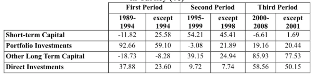
movements and also the capital flow changes, the effect of the 1994 crisis is seen on short term capital movements. The determining effect of the 1998 Asian crisis is also seen in portfolio investments. The most determining effect of the 2001 crisis is on short term capital and portolio investments. In the first two periods, while the share of short term capital and portfolio investments in total capital movements increases, the share of the other long term and direct investments decreases. In the third period, it is seen that the other long term capital flows and the direct investments increase much more significantly than the previous periods.
Table 1. Share of the Net Capital Inflows within Net Total Capital Movements in Turkey (%)
First Period Second Period Third Period 1989- 1994 except 1994 1995- 1999 except 1998 2000- 2008 except 2001 Short-term Capital -11.82 25.58 54.21 45.41 -6.61 1.69 Portfolio Investments 92.66 59.10 -3.08 21.89 19.16 20.44 Other Long Term Capital -18.73 -8.28 39.15 24.94 85.93 77.53 Direct Investments 37.88 23.60 9.72 7.74 58.56 50.15
4. Econometric Metholodogy and Data
Threshold cointegration method was introduced by Balke and Fomby (1997) by considering the long term nonlinear adjustments by combining nonlinear structure and cointegration. In the traditional approach, depending on the sign of error correction term and its statistical meaningfulness, there always occurs a trend towards the long term equilibrium point. Balke and Fomby (1997) stated that this trend would not always occur because of the costs chain that emerged in the decision stage of the economic units depending on the adaptation. Since the reactions the variables to be analysed with this thought show would be different from each other according to the economical conditions, threshold cointegration method, developed by Hansen and Seo (2002, hereafter HS), was used in this study by considering the possibility of a nonlinear relationship between savings and investments. Analysis was conducted by considering cointegrated vector whose HS method was unknown. HS developed VECM model that makes the testing of the threshold effect based on error correction term with a single cointegrated vector by means of LM test possible. The model is also called as two-regime threshold integration model or nonlinear VECM model. The predictions made based on the tests depending on the threshold cointegration analysis enables to reflect long-term relationships between the variables in a better way (Esteve et al. 2006:1036).
HS method considers that the system constructed exhibits a nonlinear tendency towards the long-term equilibrium with the assumption of the existence of two different regimes (Hansen and Seo, 2002:293). SupLM test is used in order to test the existence of threshold effect. The SupLM test, suggested by Davies (1987), Andrews (1993), Andrews and Ploberger (1994), tests the hypothesis stating “it has no threshold effect” or “it is linear”. The model used while null hypothesis is correct or there is no threshold effect is classic VECM. If threshold value parameters are defined under null hypothesis or are not determined, the result is estimated according to SupLM test. Besides, in HS test, a structure that permits structural changes in terms of parameters in addition to the error correction model of Seo (1998) is used.
In xt p magnitude I(1) is stationary and integrated with the cointegrated vector in
1
px
β
dimension. wt( )β =β′xt and is stationary in I(0) level, gives error correction term. Linear VECM model can simply be written from (l+1) degree as follows;( ) 1
xt Akxp′ Xt β ut
Δ = − + (1)
Here Xt′−1( )β kx1=
1 wt−1( )β Δxt−1 Δxt−2 . . . Δxt l−
′ -it is a vector in this magnitude- and k= pl+2. Also, it is the Martingale difference sequence that assumes that the next value of the covariance matrix Σ =E u u( t t′) limited with the error termu
twill be equal to its value again. If the threshold variable value isw
t−1, the threshold parameter can be bigger or smaller than theγ
value. With the extension of Model 1, the two regime threshold cointegration model can be denoted as follows: ( ) if ( ) , 1 1 1 ( ) if ( ) 2 1 1 A Xt ut wt xt A X u w t t t β β γ β β γ ′ − + − ≤ Δ = ′ − + −
Here γ denotes the threshold value parameter. If the model is written again according to threshold value parameter, we obtain the equation
( ) ( , ) ( ) ( , )
1 1 1 2 1 2
xt A X′ t β dt β γ A X′ t β d t β γ ut
Δ = − + − + (2)
Hansen-Seo try to calculate the
β
values in the equality no 2 assuming that p=2 and there is one cointegrated vector.Here, 1 ( , ) 1( 1( ) ) ( , ) 1( ( ) ) 2 1 dt wt d t wt β γ β γ β γ β γ = − ≤ = − .
The two-regime threshold value model (equality no 2) is defined with the error correction term. 1A and 2A coefficient matrices contain regime dynamics. β vector is standardized in order to eliminate the determination problem. Thus, the equality no 2 enables all the coefficients except cointegration vector β to transfer between two regimes. Threshold effect is valid only if 0 (P wt−1≤ γ) 1. With the re-arrangement of this constraint depending on the trimming value (0.05= 0π )5, it has
the inequality:
0
P w
(
t 1) 1
0π
≤
−≤
γ
≤ −
π
(3)With the assumption that error terms are distributed normally, the regime no (2) can be estimeated under the maximum likelihood method as follows:
1 1 ( ,1 2, , ) log ( ,1 2, , ) ( ,1 2, , ) 1 2 2 n n In A A u A At u A At t β γ = − − β γ ′− β γ = Here, the equation is,
( ,1 2, , ) 1 1( ) 1 ( , ) 2 1( ) 2 ( , )
u A At β γ = Δ −xt A X′ t− β dt β γ −A X′ t− β d t β γ
ˆ
ˆ ˆ ˆ ˆ
( ,A A1 2, , , )β γ Maximum likelihood values can be obtained by maximizing the
( ,A A1 2, ) values. If the limited maximum likelihood values for ( ,A A1 2, )
parameters are computed with OLS:
1 ˆ ( , ) (1 1( ) 1( ) 1( , )) ( 1( ) 1( ) 1( , )) 1 1 n n A Xt Xt dt Xt xt dt t t β γ = − β − β ′ β γ − − β Δ ′− β ′ β γ = = (4) 1 ˆ ( , ) (2 1( ) 1( ) 2 ( , )) ( 1( ) 1( ) 2 ( , )) 1 1 n n A Xt Xt d t Xt xt d t t t β γ = − β − β ′ β γ − − β Δ ′− β ′ β γ = = (5) 1 ˆ( , ) ˆ ( , ) ( , )ˆ 1 n ut ut t n β γ β γ β γ ′ = = . Probability function: ˆ ˆ ˆ ( , ) ( ( , ),1 2( , ), ( , ), , )) In β γ =In A β γ A β γ β γ β γ = log ˆ( , ) 2 2 n np β γ − − (6)
Minimization of the log ( , )ˆ β γ value in order to calculate the maximum likelihood values of ( , )β γ is possible under the ˆ ˆ 0 1 1( ) 1 0
1 n n xt t π ≤ − ′β γ≤ ≤ −π = constraint. 0
:
t t 1( )
tH
Δ =
x
A X
′
−β
+
u
(7) : ( ) ( , ) ( ) ( , ) 1 1 1 1 2 1 2 H Δ =xt A X′ t− β dt β γ +A X′ t− β d t β γ +ut (8)LM test will be applied for the Ho hypothesis that tests the linear cointegration relationship and the H1 hypothesis that tests nonlinear cointegration relationship. Besides being computed easily and suitable to boostrap, LM test is valid for the unconstrained model in which theoretical distribution is not known for the parameter estimation in probability or Wald type tests. If
β
andγ
are known, LM statistics can be computed as follows:1
ˆ ˆ ˆ ˆ ˆ ˆ
( , ) ( ( , ))1 2( , )) ( ( , )1 2( , )) ( ( , ))1 2( , ))
LM β γ =vec A β γ −A β γ ′V β γ +V β γ − vec A β γ −A β γ (9) Here ˆ ( , )V1 β γ and ˆ ( , )V2 β γ denote the Eicker-White covariance matrix elements computed for vecAˆ ( , )1 β γ and vecAˆ ( , )2 β γ . If β and γ are not known, LM statistic can be obtained from the threshold no (9) under an empty hypothesis. It cannot be computed under the assumption stating that there is null hypothesis or linear cointegration6. Because Davies (1977) showed that linear autoregressive
model includes a nonstandard distribution because of the problem of unidentifying the threshold parameter under the null hypothesis is “linear” hypothesis. For this reason, SubLM test introduced by Davies (1987) was used.
sup ( , ) SupLM LM L U β γ γ γ γ = ≤ ≤ was shown.
Here, Lγ is equal to the %
π
0 value of wt− 1 value in the constraint shown inequality (3), and
γ
U is equal to %(1-π
0) value. In literature it is a widespread idea that 0π value is different from 0 and between 0.05≤π0≤0.15 values for the test procedures to work. Asymptotic distribution belonging to the SupLM test necassary for the interval estimation is not affected by cointegration vectorβ . For this reason, it is not necessary to compute the cointegration vector for the tests aiming at finding the threshold value. In addition, whenβ vector is computed, it is not known what the asymptotic distribution for the SupLM test. Therefore, the critical values computed for the asymptotic distribution are obtained by the fixed variable boostrap method. When the distribution is not known, residual boostrap is applied (Rapsomanikis and Hallam, 2006:4).4.1. Data
In this study, first of all, a nonlinear relationship between the FH puzzle and the related variables are handled, test results are revised in line with the findings obtained and cointegration analysis taking the other test methods single and two-break into consideration were used7. The variables used in the study are annual and
they cover the period 1968-2008. Data set was compiled from the World Bank WDI database. Before mentioning the empirical findings, the determination and application results of the deterministic and stochastic components are given in Appnedix 2- Appnedix 5 as classical and break unit root tests.
6 It is assumed that the relationship between the variables is perfect and the cointegrated vector is [1 1] 7 The two-break unit root test of Lumsdaine and Papell (1997), the single-break unit root test of Zivot-Andrews (1992) and the multiple break unit root test of Bai-Peron (2003) is examined in this study.
5. Empirical Results
5. 1. Two-Regime Threshold Cointegration and Auto-regression (TAR) Models In this study, as in FH (1980) studies, the following model was constructed:
I Y i
= S Y i α β+
+ε
i (10)Where, I is domestic investments; S National savings; Y GDP and
ε
error term. According to Feldstein Horioka, when capital has international mobility, “there willbe no relationship between domestic savings and domestic investments. Because while in the countries with perfect capital mobility domestic investments are financed by the worldwide capital pool, domestic savings will go abroad in order to evaluate the attractive investment possibilities worldwide” (Feldstein and Horioka
(1980: 317). Thus, they argued under the assumption of FH full capital mobility that the share of savings and investments within GDP was not interrelated (β =0). Feldstein-Horioka assumed that the value of the coefficient β in the regression no (10) provided the degree of capital mobility. Accordingly, high value of β shows low capital mobility and low value shows high capital mobility. On the other hand, if capital flows are prevented due to the portfolio preferences and corporate restrictions, the increase in domestic savings will primarily reflect to the additional domestic investments (Feldstein and Horioka, 1980:328).
FH puzzle was tested with Hansen-Seo method by primarily considering a nonlinear relationship among the related variables. The estimation findings obtained according to the threshold cointegration method developed by Hansen-Seo are shown in Table 2.
Table 2. HS Test Statistics Results Lagrange Multipler Threshold Test
Test Statistic 9.95716
Fixed Regressor (Asymptotic) 5% Critical Value 16.4373 Bootstrap 5% Critical Value 16.4159 Fixed Regressor (Asymptotic) P-Value 0.780000 Bootstrap P-Value 0.800000 According to the test results, since 9.95, which was obtained, as a value of SupLM statistics was too low when compared to fix and residual bootstrap probability value, the existence of threshold cointegration was rejected. Additionally, the long-term reaction of the coefficients belonging to the variables according to the threshold value parameter is shown in Appnedix 1. When test statistics values in Table 2 are considered, the reaction of the variables in Appnedix 1 to threshold value parameter in typical and extreme regime is statistically non-significant. Accordingly, the findings obtained can be evaluated as evidence showing that there is a long-term relationship in the linear structure among the related variables. For this purpose, considering the effect of structural transformations in the Turkish economy, the existence of a long-term relationship between the variables including investments and savings was tested with Gregory- Hansen (1996), Hatemi-J (2008) regime change models, which takes single and double break into consideration.
5.2. Single and Double Break Regime Shift Models
The test carried out when structural changes in time series are not considered does not only constitute a unit root problem but it can also invalidate cointegration test results (Leybourne and Newbold, 2003). Therefore, analyses that consider whether the structural change process in time series have an effect on the degree of cointegration enable to make more efficient estimations. The most important point in FH Hypothesis is the unchangeably of political regime change in the relationship between domestic savings and investments. When this situation is considered, the problem can be in the direction that S-I relationship is not cointegrated in the long term against the political regime changes towards capital mobility and international financial integration. As Özmen and Parmaksız (2003) point out, there is no reason for a parameter assumption in different time periods in a world where capital movements have increased for the last thirty years. If the so-called regime change constitutes the centre of the problem, combining S-I relationship with an endogenous structural break analysis will be important to get more reliable results. Therefore, in this study, Gregory-Hansen (1996) test, which has been commonly used during the last period, and Hatemi-J (2008) test which is new and developed a double break cointegration test, were used?
Gregory-Hansen cointegration test is an approach that provides estimations under the break of cointegration vector and determines the break internally depending on the observation values in the system. Gregory-Hansen stated modified ADF and Za and Zt test procedures based on residuals by considering the studies of Engle and Granger (1987) and Phillips (1987) in order to test the long term relationships in case of the existence of a single break within the system. This test tests the existence of cointegration vector under a single break. Generally, the trend of the series changing depending on the time will not be modeled in this study in order to test whether the series consisting of break act together in the long term8. Because as
stated by Zivot-Andrews (1992), while the possibility of occurrence of the problematic parameters due to the oversimplification of asymptotic distribution increases, as stated in Hansen-Seo (2002), break in the trend gains a meaning when the time and size of break is only random. Because of these reasons, Gregory and Hansen formed a general model that gives permission to break in the trend and consisting of the effect of the break in the trend for cointegration vector to the break in the constant and slope (regime shift=constant break+break in the slope). The efficiency of estimation findings obtained as a result of cointegration is put forward with the help of Gregory-Hansen test. Here, it is put forward whether there is a regime shift during the concerned period depending on whether parameter estimations change along with the estimation of break year. Accordingly, the model consisting regime change can be formed as follows.
( /It GDPt)=α0+α1 1,D t+β0′(S GDPt/ t)+β1 1,′D t(S GDPt/ t)+ut (11) The artificial variable 1,D t in Model 1 shows the shifts in the constant and slope during a process of structural change and is defined as follows.
8 With the thought that the existence and effect of structural change process can be statistically significant, the procedure considering the breaks in the trend, trend + constant, trend + slope and trend + constant + slope was written by us.
[ ]
[ ]
0 if 1, 1 if t n D t = t ≤ nττ >
(12)Where,
τ
takes a value between the interval (0,1) and shows the time of breaking period. For eachτ
value of Model 1, first-degree autocorrelation coefficient is obtained by obtaining residuals under LSM (the least Squares Method).1 ˆ , ˆ , 1 1 ˆ 1 2 ˆ , 1 n e et t t n e t t τ τ ρτ τ − + = = − = (13)
Due to the fact that the sample size was not big enough, Philips (1987) Z and modified ADF test statistics by using theρτ value in a corrected form as weighted ˆ
aggregates of autovariations are shown below.
* ˆ inf ( ), ( ) ( 1) * 2 ˆ 1 2 ˆ ˆ inf ( ), ( ) , 1 2 ˆ ˆ , 1 ˆ inf ( ), ( ) ( 1 ) Z Z Z n T Zt Zt Zt s n T st et t
ADF ADF ADF t istatistik et T τ τ ρ α τ α α τ ρτ στ τ τ τ τ τ τ τ τ τ ∗ = = − ∈ − ∗ = = = − ∈ = ∗ = = − − ∈ (14)
The break in the cointegration vector and the movement of series can be observed in the long term by comparing these statistics computed from residuals with the Gregory-Hansen (1996: 559) table values.
Besides, the effect of cyclical fluctuations in the developing country economies causes a more than one structural changes in the series. When viewed in this respect, the existence of more then one breaks in the cointegration vector can change the long-term relationship of the series. This situation was included in the literature as Hatemi-J (2008) test and is an extension of Gregory-Hansen test. Only critical values and test statistics in equation 14 change. Accordingly, the related statistics were revised in equations 15 in Hatemi-J study and the regime change model, which shows the change in the constant and slope were modeled as in equation 16.
inf ( ,1 2) ( , )1 2 inf ( ,1 2) ( , )1 2 inf ( ,1 2) ( , )1 2 Z Z T Zt Zt T ADF ADF T τ τ α τ τ α τ τ τ τ τ τ τ τ ∗ = ∈ ∗ = ∈ ∗ = ∈ (15) / 0 1 1, 2 2, 0( / ) 1 1, ( / ) 2 2, ( / ) I GDPt t= +α αD t+α D t+β′ S GDPt t +β′D t tS GDPt +β′D t tS GDPt +ut (16)
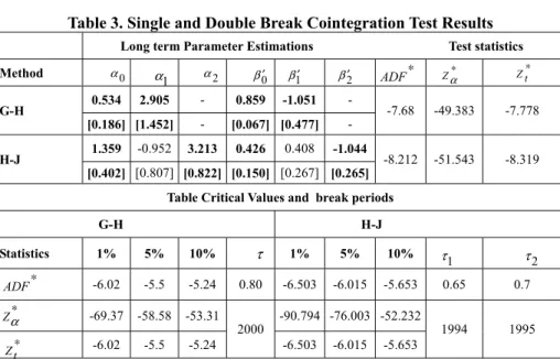
Accordingly, Gregory-Hansen and Hatemi-J single and double-break cointegration test results are shown in Table 3.
Table 3. Single and Double Break Cointegration Test Results Long term Parameter Estimations Test statistics Method
G-H 0.534 2.905 - 0.859 -1.051 - -7.68 -49.383 -7.778 [0.186] [1.452] - [0.067] [0.477] -
H-J 1.359 -0.952 3.213 0.426 0.408 -1.044 -8.212 -51.543 -8.319 [0.402] [0.807] [0.822] [0.150] [0.267] [0.265]
Table Critical Values and break periods G-H H-J Statistics 1% 5% 10% 1% 5% 10% -6.02 -5.5 -5.24 0.80 -6.503 -6.015 -5.653 0.65 0.7 -69.37 -58.58 -53.31 2000 -90.794 -76.003 -52.232 1994 1995 -6.02 -5.5 -5.24 -6.503 -6.015 -5.653
According to the Gregory-Hansen single-break cointegration test results, the saving-retention coefficient is 0.859. This coefficient showed a decrease of -1.051 units after the break year 2000. The coefficient obtained is close to 1. This situation shows when single break Gregory-Hansen test is considered that FH puzzle is going on. According to the results of Hatemi-J test, the investment-retention coefficient was found to be 0.426 until the year 1994, which was known as structural break. Structural break years were determined to be 1994 and 1995. According to the findings obtained, coefficient value between the periods of 1994-1995 increased 0.408 unit; after 1995 it decreased 1.044 unit. When the results are compared, it is seen that Hatemi-J test results, which corresponds to the literature, provides more reliable findings. When the two structural breaks are considered, it is seen that FH puzzle was eliminated. The decrease in this coefficient after break is in harmony with the idea stating that capital movements in Turkey are getting more and more integrated. Even, according to Gregory-Hansen test, it can be said that the situation showing that the coefficient value of
β
1′
(-1.051), which obtained after break, is higher when compared to H-J (-1.044) provides information expressing that the post-2000 period of capital mobility within the period it was handled has accelerated. Therefore, according to Feldstein Horioka, it can be said that, in a world where capital mobility exists, the hypothesis stating, “There will be no relationship between domestic savings and domestic investments” is valid for Turkey. Particularly, when the double structural break cointegration model is considered, it is seen that FH puzzle was eliminated in harmony with the data related to capital mobility.6. Conclusion
In this article we study the relationship between savings and investments for Turkey during the period 1968-2008 emprically with the hypothesis introduced in the original article by FH. We use two different methods in estimating the mentioned
0 α α2 β0′ β1′ β2′ ADF ∗ Zα∗ Z t∗ τ τ1 τ2 ADF ∗ Zα∗ Zt∗ 1 α
relationship: Threshold cointegration estimation method (HS) and cointegration method taking one and two regime (Hatemi-J) endogenous structural break into consideration.
In light of the findings obtained, according to the threshold estimation method which takes nonlinear structure into consideration, it was deduced that there is no nonlinear relationship between the two variables. This finding convinced people that there might be a linear relationship; then, we apply one and two structural break cointegration tests. According to single structural break cointegration model, the saving-retention coefficient got a value close to 1 and it was understood that FH puzzle continued. In the context of FH hypothesis, especially when two-structural break test was applied, the saving-retention coeficient (0.426) shows that there is capital mobility in Turkey and it increases in years. This is a very reasonable result. 1994 and 1995, which are determined as the two break years, are the years when there was financial crisis in Turkey and rapid capital escape. The results of the analysis indicate that the saving-retention coefficient increased between these two break years and decreased again after the year 1995. This means that capital mobility increases in time. When the data of Turkey regarding total capital movements are examined, after a total of 4.2 billion dollars capital outflow during the 1994 crisis, there was the same amount (4.6 billion dollars) of capital inflow in 1995 and it increased in years except 1998, 2001 and 2002. If the 1998 Russian crisis and 2001 February crisis are taken into consideration, the results are very reasonable.
The results obtained indicate that in testing the FH hypothesis for Turkey or any sample country during the concerned period, applying test techniques that take endogenous structural breaks into consideration instead of a fixed parameter hypothesis can give more reliable results. These result can lead to a beter understanding of the saving-retention coefficient in future research.
7. References
ADEDEJI, O., THORNTON, J. (2008). International capital mobility: evidence from panel cointegration tests. Economic Letters, 99 (2), 349-352. pp.
ALEXAKIS, P., APERGIS, N. (1994). The Feldstein-Horioka puzzle and exchange rate regimes: evidence from cointegration Tests. Journal of Policy Modeling, 16 (5), 459-472. pp.
ANDRADE, J. S. (2008). European integration and external sustainability of the European Union: an application of the thesis of Feldstein and Horioka. Transition Studies Review, 15, 21-36. pp.
ANDREWS, D. W. K. (1993). Tests for parameter instability and structural change with unknown change point. Econometrica, 61 (4), 821-856. pp.
ANDREWS, D. W. K., PLOBERGER, W. (1994). Optimal tests when a nuisance parameter is present only under the alternative. Econometrica, 62 (6), 1383-1414. pp.
APERGIS, N., TSOULFIDIS, L. (1997). The relationship between saving and finance: theory and evidence from EU countries. Research in Economics, 51 (4), 333-358. pp.
BAI, J., PERRON, P. (2003). Computation and analysis of multiple structural change models. Journal of Applied Econometrics, 18, 1-22. pp.
BAJO-RUBIO, O. (1998). The saving-investment correlation revisted: the case of Spain, 1964-1994. Applied Economics Letters, 5, 769-772. pp.
BALKE, N., FOMBY, T. (1997). Threshold cointegration. International Economic Review, 38, 627-645. pp.
BAXTER, M., CRUCINI, M.J. (1993). Explaining saving-investment correlations. American EconomicReview, 83, 416-436. pp.
BAYOUMI, T. (1990). Saving-investment correlations: immobile capital, government policy, or endogenous behaviour? IMF Staff Papers, 37, 360-387. pp.
BORATAV, K. (2001). 2000-2001 krizinde sermaye hareketleri [capital movements during The Crisis: 2000/2001]. İktisat İşletme ve Finans, 16 (186), 7-17. pp.
CAPORALE, G.M., PANOPOULOU, E., PITTIS, N. (2005). The Feldstein-Horioka puzzle revisted: A Monte Carlo study. Journal of International Money and Finance, 24, 1143-1149. pp.
CHAN, T., BAHARUNSHAH, A.Z. (2007). Measuring capital mobility in the Asia Pacific Rim (MIPRA Paper No. 2208). Retrieved 2012, May 01, from http://mpra.ub.uni-muenchen.de/2208/
COAKLEY, J., KULASI, F., SMITH, R. (1996). Current account solvency and the Feldstein-Horioka puzzle. The Economic Journal, 106(436), 620-627. pp.
COITEUX, M., OLIVER, S. (2000). The saving retention coefficient in the long run and in the short run: evidence from panel data. Journal of International Money and Finance, 19, 535-548. pp.
DAVIES, R.B. (1977). Hypothesis testing when a nuisance parameter is present only under the alternative. Biometrika, 64 (2), 247-254. pp.
DAVIES, R.B. (1987). Hypothesis testing when a nuisance parameter is present only under the alternative. Biometrika, 74 (1), 33-43. pp.
DE VITA, G., ANDREW, A. (2002). Are saving and investment cointegrated? An ARDL bounds testing approach. Economic Letters, 177 (2), 293-299. pp.
DOOLEY, M., JEFFREY, A., MATHIESON, D. (1987). International capital mobility: saving-investment correlations tell us? IMF Staff Papers, 34 (3), 503-530. pp.
ENGLE, R.F., GRANGER, C.W.J. (1987). Co-integration and error correction: representation, estimation, and testing. Econometrica, 55 (2), 251-276. pp.
ESTEVE, V., GILL-PAREJA, S., MARTINEZ-SERRANO, A., LLORCA-VIVERO, R. (2006). Threshold cointegration and nonlinear adjustment between goods and services inflation in the United States. EconomicModelling, 23 (6), 1033-1039. pp.
FELDSTEIN, M. (1983). Domestic saving and international capital movements in the long run and the short run. European Economic Review, 21, 129-151. pp.
FELDSTEIN, M., BAACHETTA, P. (1989). National saving and international investment. NBER WorkingPaper, 3164, 1-37. pp.
FELDSTEIN, M., HORIOKA, C. (1980). Domestic saving and international capital flows. The Economic Journal, 90 (358), 314-329. pp.
GREGORY, A.W., HANSEN, B.E. (1996). Residual-based tests for cointegration in models with regime shifts. Journal of Econometrics, 70 (1), 99-126. pp.
GUNDLACH, E., SINN, S. (1992). Unit root tests of the current account balance: implications for international capital mobility. Applied Economics, 24 (6), 617-625, pp. HANSEN, B., SEO, B. (2002). Testing for two-regime threshold cointegration in vector
error-correction models. Journal of Econometrics, 110, 293-318. pp.
HATEMI-J, A. (2008). Tests for cointegration with two unknown regime shifts with an application to financial market integration. Empirical Economics, 135 (3), 497-505. pp. HO, T. W. (2002). A panel cointegration approach to the investment-saving correlation.
Empirical Economics, 27, 91-100. pp.
HOGENDORN, C. (1998). Capital mobility in historical perspective. Journal of Policy Modeling, 20 (2), 141-161. pp.
INSEL, A., SUNGUR, N. (2003). Sermaye akımlarının temel makroekonomik göstergeler üzerindeki etkileri: Türkiye örneği-1989: III-1999:IV. Türkiye Ekonomi Kurumu, Tartışma Metni 2003/8. [Available at]: < http/www.tek.org.tr >, [Accessed: 01.05.2012]. JANSEN, W. J. (1996). Estimating saving-investment correlations: evidence for OECD countries based on an error correction model. Journal of International Money and Finance, 15, 749-781. pp.
KAYA-BAHCE, S., OZMEN, E. (2008). Exchange rate regimes, saving glut and the Feldstein-Horioka puzzle: The East Asian experience. Physica A, 387, 2561-2564. pp. LEYBOURNE, S., NEWBOLD, P. (2003). Spurious rejections by cointegration tests induced
LUMSDAINE, R.L., PAPEL, D.H. (1997). Multiple trend breaks and the unit-root hypothesis. The Review of Economics and Statistics, 79 (2), 212-218. pp.
MORENO, R. (1997). Saving-investment dynamics and capital mobility in the US and Japan. Journal of International Money and Finance, 16 (6), 837-863. pp.
MURPHY, R.G. (1984). Capital mobility and relationship between saving and investment rates. Journal of International Money and Finance, 3 (3), 327-342. pp.
NARAYAN, P.K. (2005). The relationship between saving and investment for Japan. Japan and the World Economy, 17, 293-309. pp.
OBSTFELD, M. (1994). International capital mobility in the 1990s (International Finance Discussion Papers No. 472). [Available at]: < http://www.federalreserve.gov/Pubs/Ifdp/ 1994/472/ifdp472.pdf>, [Accessed: 01.05.2010].
OZMEN, E., PARMAKSIZ, K. (2003). Policy regime change and Feldstein-Horioka puzzle: The UK evidence. Journal of Policy Modeling, 25, 137-149. pp.
PELAGIDIS, T., MASTROYIANNIS, T. (2003). The saving-investment correlation in Greece, 1960-1997: implications for capital mobility. Journal of Policy Modeling, 25, 609-616. pp
PHILLIPS, P. (1987). Time series regression with a unit root. Econometrica, 55, 277-301. pp. RAPSOMANAKIS, G., HALLAM, D. (2006). Threshold cointegration in the sugar-ethanol-oil price system in Brazil: evidence from nonlinear vector error corrections model (Fao Commodity and Trade Policy Research Working Paper No. 2). [Available at]: <ftp://ftp.fao.org/docrep/fao/009/ah471e/ah471e00.pdf >, [Accessed: 27.06.2010]. SACHSIDA, A., CAETANO, M.A. (2000). The Feldstein-Horioka puzzle revisted.
Economic Letters, 68, 85-88. pp.
SEO, B. (1998). Tests for structural change in cointegrated systems. Econometric Theory, 14 (2), 222-259. pp.
SINHA, T., SINHA, D. (1998). Cart before the horse? The saving-growth nexus in Mexico. Economic Letters, 61 (1), 43-47. pp.
SINHA, T., SINHA, D. (2004). The mother of all puzzles would not go away. Economic Letters, 82 (2), 259-267. pp.
TELATAR, E., TELATAR, F., BOLATOĞLU, N. (2007). A regime switching approach to the Feldstein-Horioka puzzle: evidence from some European Countries. Journal of Policy Modeling, 29, 523-533. pp.
TESAR, L.L. (1991). Saving, investment, and international capital flows. Journal of International Economics, 31 (1-2), 55-78. pp.
TESAR, L.L. (1993). International risk-sharing and non-traded goods. Journal of International Economics, 35 (1-2), 69-89. pp.
YENTURK, N., ULENGIN, B., CIMENOGLU, A. (2007). An analysis of the Interaction among Savings and Investment and Growth in Turkey. Applied Economics, 41, 739-751. pp.
YILDIRIM, J. (2000). Current account imbalances and intertemporal approach to the balance of payments. Dokuz Eylül Üniversitesi Sosyal Bilimler Enstitüsü Dergisi, 2 (4), 122-132. pp.
ZIVOT, E., ANDREWS, W.K. (1992). Further evidence on the great crash, the oil-price shock, and the unit-root hypothesis. Journal of Business and Economic Statistics, 10 (3), 251-270. pp.
Appnedices
Appnedix 1. Response To Error Correction Coefficient of I/Y and S/Y
Appnedix 2. Unit Root Analysis
Variables Degree Level Difference Level Constant Constant+Trend Constant Constant+Trend I/GDP -1.854229 -1.378012 -5.25623 -5.384291 S/GDP -1.247373 -2.893056 -5.30425 -5.228223 %1 Difference stationary
Appnedix 3. Lumsdaine-Papell Two-Break Unit Root Test
Variable TB1 1 2 1 1 k yt t DU t DU t yt c yi t i t i μ β θ ω α ε Δ = + + + + − + Δ − + = (Model AA) TB2 α Θ ψ ω
γ
μ βτ k I/GDP 1986 -0.8671 6.4651 - -6.5769 - 12.4469 0.0812 1 t-statistics 2000 -7.6109 5.6257 - -5.7000 - 7.7681 1.4773 S/GDP 1986 -1.1435 8.5302 - -3.2051 - 13.1031 0.1357 1 t-statistics 1995 -7.8885 6.0519 - -3.5053 - 7.5206 2.4149 1 1 2 2 1 1 k yt t DU t DT t DU t DT t yt c yi t i t i μ β θ γ ω ψ α ε Δ = + + + + + + − + Δ − + = (Model CC) I/GDP 1986 -0.8647 6.6810 0.0088 -5.7578 -0.1248 12.0078 0.1267 1 t- statistics 2000 -6.9564 5.6854 0.0363 -4.1693 -1.1185 6.8269 1.8583 S/GDP 1986 -1.2046 11.0771 1.1600 -0.4166 -0.7012 13.8844 0.1332 1 t- statistics 2002 -9.2323 7.7385 3.6038 -4.3359 -0.5391 8.4940 2.1583 1 1 2 1 1 k yt t DU t DT t DU t yt c yi t i t i μ β θ γ ω α ε Δ = + + + + + − + Δ − + = (Model CA) I/GDP 1985 -0.8775 6.9214 - -6.0261 -0.0851 12.2827 0.1123 1 t- statistics 1999 -6.4716 5.5324 - -3.4799 -0.6763 6.5085 1.4375 S/GDP 1985 -1.1649 11.3418 - -0.3088 -0.2068 13.7439 0.0769 1 t- statistics 2004 -9.9305 8.7490 - -3.8762 -0.2558 9.3374 1.3086 P.S.: Critical values for model AA in the significance levels of 1%, 5% and 10% are 6.94, 6.24 and 5.96 respectively. Critical values for model CC in the significance levels of 1%, 5% and 10% are 7.34, -6.82 and -6.49 respectively. Similarly, critical values for model CA in the significance levels of 1%, 5% and 10% are -7.24, -6.65 and -6.33 respectively.Appnedix 4. Zivot-Andrews Single-Break Unit Root Test
Variables Constant Trend Constant+Trend
I/GDP -3.231*** -3.007 -4.900***
S/GDP -4.789*** -2.956 -5.073***
P.S.: *** indicates that the related test statistic is different from zero in the significance level of 10%. Appnedix 5. Bai-Peron Multiple Break Unit Root Test
zt{1} q=1 p=0 h=6 M=5 Double Max Tests
I/GDP
SupFt(1) SupFt(2) SupFt(3) SupFt(4) SupFt(5) UDmax WDmax 3.7660 49.8630* 45.6944* 42.6230* 36.4194* 49.8630* 73.8883*
SupF(2|1) SupF(3|2) SupF(4|3) SupF(5|4)
64.5091 4.6069 1.4217 0.1172
The number of breaks according to information criteria Sequential -
LWZ 3
BIC 3
Estimation with double breaks (BIC)
δ1 δ2 δ3 δ4 T1 T2 T3
13.040251 15.881297 24.234320 17.419602 1980 1986 2000 1.0232 0.7216 0.5439 0.5989 [1968-1982] [1985-1988] [1999-2001]
S/GDP
SupFt(1) SupFt(2) SupFt(3) SupFt(4) SupFt(5) UDmax WDmax 91.3597* 56.0324* 52.8138* 56.4634* 43.2358* 91.3597* 91.3597*
SupF(2|1) SupF(3|2) SupF(4|3) SupF(5|4)
2.2904 2.2904 2.2904 0.2505
The number of breaks according to information criteria Sequential 1
LWZ 1
BIC 1
Estimation with double breaks (LWZ)
δ1 δ2 T1
12.442503 20.850877 1986
0.4161 0.7503 1984-1987
Appnedix 6. Net Capital Flows in Turkish Economy: 1980-2008 (billion dollars) Short term
Capitala Investments Portfolio term Capital Other Long a Investments Direct Total Capital Movements
1980 -2 0 656 18 672 1981 121 0 683 95 899 1982 98 0 127 55 280 1983 798 0 39 46 883 1984 -652 0 612 113 73 1985 1479 0 -513 99 1065 1986 812 146 1041 125 2124 1987 50 282 1453 106 1891 1988 2281 1178 -209 354 -958 1989 -584 1386 -685 663 780 1990 3000 547 -210 700 4037
Appnedix 6. Continue 1991 -3020 623 -783 783 -2397 1992 1396 2411 -938 779 3648 1993 3054 3917 1370 622 8963 1994 -5127 1158 -784 559 -4194 1995 3713 237 -79 772 4643 1996 5945 570 1636 612 8763 1997 1761 1634 4788 554 8737 1998 2601 -6711 3985 573 448 1999 759 3429 345 138 4671 2000 4174 1022 4276 112 9584 2001 -11766 -4515 -1131 2855 -14557 2002 -1279 -593 2105 939 1172 2003 4.283 2465 -808 1252 7192 2004 1509 8023 6165 2005 17702 2005 6954 13437 13302 8967 42660 2006 -10557 7373 26612 19261 42689 2007 -4233 717 32213 19940 48637 2008 2610 -4778 21062 15400 34294
Source: CBT (Central Bank of Turkey), Statistics on Balance of Payments a Including the suitcase trading since 1996.