Discrete pseudo-SINR-balancing nonlinear recurrent system

(1)

Volume 2013, Article ID 480560,19pages http://dx.doi.org/10.1155/2013/480560

Research Article

Discrete Pseudo-SINR-Balancing Nonlinear Recurrent System

Zekeriya Uykan

1,2

1_{Control and Automation Engineering Department, Do˘gus¸ University, Acibadem, Kadikoy, 34722 Istanbul, Turkey} 2_{Aalto University School of Electrical Engineering, Department of Communications and Networking (COMNET),}

PL 13000 Aalto, 00076 Espoo, Finland

Correspondence should be addressed to Zekeriya Uykan; zuykan@dogus.edu.tr Received 24 October 2012; Revised 7 February 2013; Accepted 5 March 2013 Academic Editor: Kwok-Wo Wong

Copyright © 2013 Zekeriya Uykan. This is an open access article distributed under the Creative Commons Attribution License, which permits unrestricted use, distribution, and reproduction in any medium, provided the original work is properly cited. Being inspired by the Hopfield neural networks (Hopfield (1982) and Hopfield and Tank (1985)) and the nonlinear sigmoid power control algorithm for cellular radio systems in Uykan and Koivo (2004), in this paper, we present a novel discrete recurrent nonlinear system and extend the results in Uykan (2009), which are for autonomous linear systems, to nonlinear case. The proposed system can be viewed as a discrete-time realization of a recently proposed continuous-time network in Uykan (2013). In this paper, we focus on discrete-time analysis and provide various novel key results concerning the discrete-time dynamics of the proposed system, some of which are as follows: (i) the proposed system is shown to be stable in synchronous and asynchronous work mode in discrete time; (ii) a novel concept called Pseudo-SINR (pseudo-signal-to-interference-noise ratio) is introduced for discrete-time nonlinear systems; (iii) it is shown that when the system states approach an equilibrium point, the instantaneous Pseudo-SINRs are balanced; that is, they are equal to a target value. The simulation results confirm the novel results presented and show the effectiveness of the proposed discrete-time network as applied to various associative memory systems and clustering problems.

1. Introduction

Artificial neural networks have been an important research area since 1970s. Since then, various biologically inspired neu-ral network models have been developed. Hopfield Neuneu-ral Networks [1,2] have been one of the most widely used neural networks since the early 1980s whose applications vary from combinatorial optimization (e.g., [3,4]) to image restoration (e.g., [5]) and from various control engineering optimization problems in robotics (e.g., [6]) to associative memory systems (e.g., [7, 8]). For a tutorial and further references about Hopfield neural networks, see, for example, [9,10].

In [11], we introduce a novel pseudo-signal-to-interfer-ence-noise ratio concept for discrete-time autonomous linear systems. Our main motivation in this paper is to investigate a nonlinear extension of [11]. Furthermore, the proposed system can be viewed as a discrete-time realization of a very recently proposed continuous-time network called double-sigmoid continuous-time Hopfield neural network in a brief letter [12]. And our investigations in this paper yield various interesting key novel results in discrete time, some of which

are as follows: (i) a novel concept called Pseudo-SINR (pseudo-signal-to-interference-noise ratio) is introduced for discrete-time nonlinear systems; (ii) it is shown that when the network approaches to one of its equilibrium points, the instantaneous Pseudo-SINRs are balanced; that is, they are equal to a target value; (iii) the proposed network outperforms its Hopfield neural network counterpart as applied to various associative memory systems and clustering applications. The disadvantage of the proposed network is that it increases the computational burden.

The paper is organized as follows. The proposed recurrent network and its stability features are analyzed inSection 2. Simulation results are presented in Section 3, followed by conclusions inSection 4.

2. Discrete Pseudo-SINR-Balancing Recurrent

Neural Networks

Being inspired by the nonlinear sigmoid power control algorithm for cellular radio systems in [13] and the Hopfield

(2)

neural networks [2], we propose the following discrete nonlinear recurrent network:

x(𝑘 + 1) = x (𝑘) + 𝛼 (𝑘) f1(−Ax (𝑘) + W𝑓2(x (𝑘)) + b) , (1) where 𝑘 represents the iteration step, A, W, and b are defined as in (2), and f𝑚(⋅), 𝑚 = 1, 2, represents a vectoral mapping from R𝑁 to R𝑁. For an 𝑁-dimensional vector

e = [𝑒1𝑒2⋅ ⋅ ⋅ 𝑒𝑁]𝑇, f𝑚(e) = [𝑓𝑚(𝑒1)𝑓𝑚(𝑒2) ⋅ ⋅ ⋅ 𝑓𝑚(𝑒𝑁)]𝑇where

𝑓_𝑚(⋅) is chosen as the sigmoid function; that is, for a real number𝑒_𝑖, the output is𝑓_𝑚(𝑒_𝑖) = 𝜅_𝑚(1−(2/(1+exp(−𝜎_𝑚𝑒_𝑖)))), where 𝜅_𝑚 > 0, 𝜎_𝑚 > 0. We will call the network in (1) as discrete sigmoid-pseudo-SINR-balancing recurrent neural network (D-SP-SNN). The name comes from the fact that the proposed network balances an entity called Pseudo-SINR, as will be seen in the following. In this paper, we choose sigmoid function because it’s used both in Hopfield neural network and the power control algorithm in [13]. Furthermore, the proposed D-SP-SNN can be viewed as a discrete-time implementation of a very recently proposed time network called double-sigmoid continuous-time Hopfield neural network in the brief [12]. In this paper, we focus on discrete-time analysis and provide various novel key results concerning the discrete-time dynamics of the proposed system: A = [ [ [ [ [ 𝑎₁₁ 0 ⋅ ⋅ ⋅ 0 0 𝑎₂₂ ⋅ ⋅ ⋅ 0 .. . d 0 0 0 ⋅ ⋅ ⋅ 𝑎𝑁𝑁 ] ] ] ] ] , W = [ [ [ [ [ 0 𝑤12 ⋅ ⋅ ⋅ 𝑤1𝑁 𝑤21 0 ⋅ ⋅ ⋅ 𝑤2𝑁 .. . d ... 𝑤_𝑁1 𝑤_𝑁2 ⋅ ⋅ ⋅ 0 ] ] ] ] ] , b = [ [ [ [ [ 𝑏₁ 𝑏₂ .. . 𝑏_𝑁 ] ] ] ] ] . (2)

In (2), A shows the self-state-feedback matrix, W with zero diagonal shows the interneurons connection weight matrix, and b is a threshold vector.

The proposed network includes both the sigmoid power control in [13] and the traditional Hopfield neural network (HNN) as its special cases by choosing the𝑓₁(⋅) and 𝑓₂(⋅) appropriately. The Euler approximation of the continuous-time HNN is given as

x(𝑘 + 1) = x (𝑘) + 𝛼 (𝑘) (−Ax (𝑘) + W𝑓2(x (𝑘)) + b) . (3)

Let us call the network in (3) HNN-Euler, which is a special case of the proposed D-SP-SNN in (1). From (1),

𝑥_𝑗(𝑘 + 1) = 𝑥_𝑗(𝑘) + 𝛼 (𝑘) × 𝑓₁(−𝑎_𝑗𝑗𝑥_𝑗(𝑘) + 𝑏_𝑗+ ∑𝑁 𝑖=1,𝑖 ̸= 𝑗 𝑤_𝑖𝑗𝑓₂(𝑥_𝑖(𝑘))) , 𝑗 = 1, . . . , 𝑁, (4) where𝛼(𝑘) is the step size at time 𝑘. Let’s define the error signal𝑒_𝑖(𝑘) as 𝑒𝑖(𝑘) = −𝑎𝑖𝑖𝑥𝑖+ 𝐼𝑖(𝑘) , where𝐼_𝑖(𝑘) = 𝑏_𝑖+ 𝑁 ∑ 𝑗=1,𝑗 ̸= 𝑖𝑤𝑖𝑗𝑓2(𝑥𝑗(𝑘)) , 𝑖 = 1, . . . , 𝑁. (5) Then, the performance index is defined as𝑙₁-norm of the error vector in (5) as follows:

𝑉 (𝑘) = ‖e (𝑘)‖1= 𝑁 ∑ 𝑖 󵄨󵄨󵄨󵄨𝑒𝑖(𝑘)󵄨󵄨󵄨󵄨 (6) =∑𝑁 𝑖 󵄨󵄨󵄨󵄨−𝑎𝑖𝑖 𝑥_𝑖+ 𝐼_𝑖󵄨󵄨󵄨󵄨, where𝐼_𝑖= 𝑏_𝑖+ 𝑁 ∑ 𝑗=1,𝑗 ̸= 𝑖 𝑤_𝑖𝑗𝑓₂(𝑥_𝑗) . (7)

In what follows, we examine the evolution of the energy function in (6) in synchronous and asynchronous work modes. Asynchronous mode means that at every iteration step, at most only one state is updated, whereas synchronous mode refers to the case that all the states are updated at every iteration step according to (4).

Proposition 1. In asynchronous mode of the proposed network

D-SP-SNN in (4) with a symmetric matrix W, for a nonzero

error vector, the𝑙₁-norm of the error vector in (6) decreases at

every step; that is, the error vector goes to zero for any𝛼(𝑘) such

that 󵄨󵄨󵄨󵄨 󵄨𝑒𝑗(𝑘)󵄨󵄨󵄨󵄨_{󵄨 >}󵄨󵄨󵄨󵄨_󵄨𝑎𝑗𝑗𝛼 (𝑘) 𝑓1(𝑒𝑗(𝑘))󵄨󵄨󵄨󵄨_󵄨 (8) if 󵄨󵄨󵄨󵄨 󵄨𝑎𝑗𝑗󵄨󵄨󵄨󵄨_{󵄨 ≥ 𝑘}2 𝑁 ∑ 𝑖=1,(𝑖 ̸= 𝑗)󵄨󵄨󵄨󵄨󵄨𝑤𝑖𝑗󵄨󵄨󵄨󵄨󵄨 , (9)

where𝑘₂ = 0.5𝜎₂ is the global Lipschitz constant of𝑓₂(⋅) as

shown the inAppendix A.

Proof. In asynchronous mode, only one state is updated at

an iteration time. Let𝑗 show the index of the state which is updated at time𝑘 whose error signal is different than zero;

(3)

that is,𝑒_𝑗= −𝑎_𝑗𝑗𝑥_𝑗+𝐼_𝑗 ̸= 0, where 𝐼_𝑗= 𝑏_𝑗+∑𝑁_{𝑖=1,𝑖 ̸= 𝑗}𝑤_𝑗𝑖𝑓₂(𝑥_𝑖), as defined in (5). Writing (5) in vector form for steps𝑘 and 𝑘 + 1 results in e(𝑘 + 1) − e (𝑘) = [ [ [ [ [ [ [ [ [ [ 0 0 .. . −𝑎_𝑗𝑗(𝑥_𝑗(𝑘 + 1) − 𝑥_𝑗(𝑘)) .. . 0 ] ] ] ] ] ] ] ] ] ] + [ [ [ [ [ [ [ [ [ [ 𝑤_1𝑗 𝑤_2𝑗 .. . 0 .. . 𝑤_𝑁𝑗 ] ] ] ] ] ] ] ] ] ] (𝑓₂(𝑥_𝑗(𝑘 + 1)) − 𝑓₂(𝑥_𝑗(𝑘))) . (10) Using the error signal definition of (5) in (4) gives

𝑥_𝑗(𝑘 + 1) − 𝑥_𝑗(𝑘) = 𝛼 (𝑘) 𝑓₁(𝑒_𝑗(𝑘)) . (11) So, the error signal for state𝑗 is obtained using (10) and (11) as follows:

𝑒_𝑗(𝑘 + 1) − 𝑒_𝑗(𝑘) = −𝑎_𝑗𝑗(𝑥_𝑗(𝑘 + 1) − 𝑥_𝑗(𝑘)) (12) = −𝑎_𝑗𝑗𝛼 (𝑘) 𝑓1(𝑒𝑗(𝑘)) . (13) From (12) and (13), if𝛼(𝑘) is chosen to satisfy |𝑒_𝑗(𝑘)| > |𝑎_𝑗𝑗𝛼(𝑘)𝑓₁(𝑒_𝑗(𝑘))|, then

󵄨󵄨󵄨󵄨

󵄨𝑒𝑗(𝑘 + 1)󵄨󵄨󵄨󵄨_{󵄨 <}󵄨󵄨󵄨󵄨_󵄨𝑒𝑗(𝑘)󵄨󵄨󵄨󵄨_{󵄨 , for} 󵄨󵄨󵄨󵄨𝑒𝑖(𝑘)󵄨󵄨󵄨󵄨 ̸= 0, (14) where𝑓₁(⋅) is a sigmoid function, which is lower and upper bounded. Since the sigmoid function𝑓₁(⋅) has the same sign as its argument and𝑓₁(𝑒_𝑗) = 0 if and only if 𝑒_𝑗 = 0, then it is seen that𝛼(𝑘) can easily be chosen small enough to satisfy |𝑒_𝑗(𝑘)| > 𝛼(𝑘)𝑎_𝑗𝑗|𝑓₁(𝑒_𝑗(𝑘))| according to the parameter 𝑎_𝑗𝑗 and the slope of sigmoid function𝑓₁(⋅).

Above, we examined only the state𝑗 and its error signal 𝑒𝑗(𝑘). In what follows, we examine the evolution of the norm of the complete error vector e(𝑘+1) in (10). From the point of view of the𝑙₁norm of the e(𝑘 + 1), the worst case is that when |𝑒_𝑗(𝑘)| decreases, all other elements |𝑒_𝑖(𝑘)|, 𝑖 ̸= 𝑗, increase. So, using (10), (12), and (14), we obtain that if

󵄨󵄨󵄨󵄨 󵄨−𝑎𝑗𝑗(𝑥𝑗(𝑘 + 1) − 𝑥𝑗(𝑘))󵄨󵄨󵄨󵄨_{󵄨 ≥}_󵄨𝑓󵄨󵄨󵄨󵄨 2(𝑥𝑗(𝑘 + 1)) − 𝑓2(𝑥𝑗(𝑘))󵄨󵄨󵄨󵄨_󵄨 × ∑𝑁 𝑖=1,(𝑖 ̸= 𝑗)󵄨󵄨󵄨󵄨󵄨𝑤𝑖𝑗󵄨󵄨󵄨󵄨󵄨 , (15) then

‖e (𝑘 + 1)‖₁{< ‖e (𝑘)‖1 if‖e (𝑘)‖1 ̸= 0,

= 0 if‖e (𝑘)‖₁= 0. (16)

The sigmoid function 𝑓₂(⋅) is a Lipschitz continuous function as shown inAppendix A. So,

𝑘₂󵄨󵄨󵄨󵄨_󵄨𝑥_𝑗(𝑘 + 1) − 𝑥_𝑗(𝑘)󵄨󵄨󵄨󵄨_{󵄨 ≥}_󵄨𝑓󵄨󵄨󵄨󵄨 ₂(𝑥_𝑗(𝑘 + 1)) − 𝑓₂(𝑥_𝑗(𝑘))󵄨󵄨󵄨󵄨_{󵄨 ,} (17) where 𝑘₂ = 0.5𝜎₂ is 𝑓₂(⋅)’s global Lipschitz constant as shown inAppendix A. From (15) and (17), choosing|𝑎_𝑗𝑗| > 𝑘₂∑𝑁_{𝑖=1,(𝑖 ̸= 𝑗)}|𝑤_𝑖𝑗| yields (15), which implies (16). This com-pletes the proof.

Definition 2 (pseudo-SINR). We define the following system

variable, which will be called pseudo-SINR, for the D-SP-SNN in (4): 𝜃_𝑖 𝜃tgt 𝑖 = 𝑎𝑖𝑖𝑓 (𝑥𝑖) 𝑏_𝑖+ ∑𝑁_{𝑗=1,𝑗 ̸= 𝑖}𝑤_𝑖𝑗𝑓 (𝑥_𝑗), 𝑖 = 1, . . . , 𝑁, (18) where𝑓(⋅) represents the sigmoid function, that is, 𝑓(𝑒) = 𝜅(1 − (2/(1 + exp(−𝜎𝑒)))), and 𝜃tgt

𝑖 is a constant, which we call target𝜃_𝑖.

Examining the𝜃_𝑖in (18), we observe that it resembles the traditional signal-to-interference-noise ratio (SINR) defini-tion in cellular radio systems (see, e.g., [14,15]); therefore we call it Pseudo-SINR.

Definition 3 (prototype vectors). Prototype vectors are

defined as those x’s which make 𝜃_𝑖 = 𝜃tgt_𝑖 , 𝑖 = 1, . . . , 𝑁, in (18). So, from (18) and (5), the prototype vectors make the error signal zero; that is,𝑒_𝑖= 0, 𝑖 = 1, . . . , 𝑁 given that 𝑥_𝑖 ̸= 0 and𝐼_𝑖 ̸= 0.

Proposition 4. In asynchronous mode, choosing the slope of 𝑓₂(⋅) relatively small as compared to 𝑓₁(⋅) and choosing 𝑎_𝑗𝑗> 0

and𝛼(𝑘) satisfying (8), the D-SP-SNN in (4) with a symmetric

matrix W is stable and there exists a finite time constant such

that the𝑙₁-norm of the error vector in (6) approaches to an

𝜖-vicinity of the zero as its steady state, where𝜖 is a relatively

small positive number. If𝜃_𝑖 = 𝜃_𝑖tgtat the converged point, then

it corresponds to a prototype vector as defined above.

Proof. Since it is asynchronous mode, (10)–(14) hold where

𝑎_𝑗𝑗 > 0. So, if 𝛼(𝑘) at time 𝑘 is chosen to satisfy |𝑒_𝑗(𝑘)| > |𝑎_𝑗𝑗𝛼(𝑘)𝑓₁(𝑒_𝑗(𝑘))| as in (8), then

󵄨󵄨󵄨󵄨

󵄨𝑒𝑗(𝑘 + 1)󵄨󵄨󵄨󵄨_{󵄨 <}󵄨󵄨󵄨󵄨_󵄨𝑒𝑗(𝑘)󵄨󵄨󵄨󵄨_{󵄨 , for} 󵄨󵄨󵄨󵄨𝑒𝑖(𝑘)󵄨󵄨󵄨󵄨 ̸= 0. (19) Note that it is straightforward to choose a sufficiently small𝛼(𝑘) to satisfy (8) according to𝑎_𝑗𝑗and the slope𝜎₁of sigmoid𝑓₁(⋅). Using (10), (12), and (19), it is seen for𝑒_𝑗(𝑘) ̸= 0 that if 󵄨󵄨󵄨󵄨 󵄨−𝑎𝑗𝑗(𝑥𝑗(𝑘 + 1) − 𝑥𝑗(𝑘))󵄨󵄨󵄨󵄨_󵄨 = 󵄨󵄨󵄨󵄨󵄨−𝑎𝑗𝑗𝛼 (𝑘) 𝑓1(𝑒𝑗(𝑘))󵄨󵄨󵄨󵄨_󵄨 (20) > 󵄨󵄨󵄨󵄨󵄨𝑓2(𝑥𝑗(𝑘 + 1)) − 𝑓2(𝑥𝑗(𝑘))󵄨󵄨󵄨󵄨_󵄨 × ∑𝑁 𝑖=1,(𝑖 ̸= 𝑗)󵄨󵄨󵄨󵄨󵄨𝑤𝑖𝑗󵄨󵄨󵄨󵄨󵄨 , (21)

(4)

then

‖e (𝑘 + 1)‖₁< ‖e (𝑘)‖1. (22) We observe from (12), (20), (21), and (22) the following. (1) If the 𝑥𝑖(𝑘), 𝑖 = 1, . . . , 𝑁, approach to either of the saturation regimes of its sigmoid function𝑓₂(⋅), then

󵄨󵄨󵄨󵄨 󵄨𝑓2(𝑥𝑗(𝑘 + 1)) − 𝑓2(𝑥𝑗(𝑘))󵄨󵄨󵄨󵄨_󵄨 𝑁 ∑ 𝑖=1,(𝑖 ̸= 𝑗)󵄨󵄨󵄨󵄨󵄨𝑤𝑖𝑗󵄨󵄨󵄨󵄨󵄨 ≈ 0, 𝑗 = 1, . . . , 𝑁, (23) since|𝑓₂(𝑥_𝑗(𝑘 + 1)) − 𝑓₂(𝑥_𝑗(𝑘))| ≈ 0, 𝑖 = 1, . . . , 𝑁. That satisfies (20) and (21). Therefore, the norm of the error vector in (6) does not go to infinity and is finite for any x.

(2) x(𝑘 + 1) = x(𝑘) if and only if e(𝑘) = 0; that is, 𝑥_𝑗(𝑘 + 1) = 𝑥𝑗(𝑘) if and only if 𝑓1(𝑒𝑗(𝑘)) = 0,

𝑗 = 1, . . . , 𝑁. (24) (3) Examining the (11), (12), and (13) taking the observa-tions(1) and (2) into account, we conclude that any of the 𝑥_𝑗(𝑘), 𝑗 = 1, . . . , 𝑁, does not go to infinity and is finite for any𝑘. So, the D-SP-SNN in (4) with a symmetric matrix W is stable for the assumptions inProposition 4. Because there is a finite number of insaturation states (i.e., the number of all possible insaturation state combinations is finite), which is equal to2𝑁, there exists a finite time constant such that the𝑙₁ -norm of the error vector in (6) approaches to an𝜖-vicinity of the zero as its steady state, where𝜖 is a relatively small positive number.

From (18), if𝜃_𝑖 = 𝜃tgt_𝑖 at the converged point, then it corresponds to a prototype vector as defined in the previous section, which completes the proof.

In what follows, we examine the evolution of pseudo-SINR𝜃_𝑖(𝑘) in (18). From (18), let us define the following error signal at time𝑘:

𝜉_𝑗(𝑘) = −𝜃_𝑗(𝑘) + 𝜃tgt

𝑗 , 𝑗 = 1, . . . , 𝑁. (25) Proposition 5. In asynchronous mode, in the D-SP-SNN in (4) with a sufficiently small𝛼(𝑘) and with a symmetric matrix

W, the 𝜃𝑗(𝑘) is getting closer to 𝜃tgt𝑗 at those iteration steps𝑘

where𝐼_𝑗(𝑘) ̸= 0; that is, |𝜉_𝑗(𝑘 + 1)| < |𝜉_𝑗(𝑘)|, where index 𝑗

shows the state being updated at iteration𝑘.

Proof. Let𝑗 show the state which is updated at time 𝑘. The

pseudo-SINR defined by (18) for nonzero𝐼_𝑗(𝑘) is equal to 𝜃_𝑗(𝑘) = 𝑎𝑖𝑖𝑥𝑗(𝑘) 𝐼_𝑗(𝑘) , where 𝐼𝑗(𝑘) = 𝑏𝑗+ 𝑁 ∑ 𝑖=1,𝑖 ̸= 𝑗 𝑤_𝑗𝑖𝑓 (𝑥_𝑗(𝑘)) . (26) Without loss of generality, and for the sake of simplicity, let is take𝜃_𝑖tgt= 1. Then, from (26) and (25)

𝜉_𝑗(𝑘) = −𝜃_𝑗(𝑘) + 1 = −𝑎𝑖𝑖𝑥𝑗_𝐼(𝑘) + 𝐼𝑗(𝑘)

𝑗(𝑘) . (27)

In asynchronous mode, from (26),𝐼_𝑚(𝑘) = 𝐼_𝑚(𝑘 + 1). Using this observation and (27),

𝜉_𝑗(𝑘 + 1) − 𝜉_𝑗(𝑘) = −𝑎𝑖𝑖(𝑥𝑗(𝑘 + 1) − 𝑥𝑗(𝑘)) 𝐼𝑗(𝑘) . (28) From (4) and (28), 𝜉_𝑗(𝑘 + 1) − 𝜉_𝑗(𝑘) = −𝑎𝑖𝑖𝛼 (𝑘) 𝑓1(𝑒𝑗(𝑘)) 𝐼_𝑗(𝑘) . (29)

Provided that𝐼_𝑗(𝑘) ̸= 0, we write, from (5) and (27), 𝑒_𝑗(𝑘) = 𝐼_𝑗(𝑘) 𝜉_𝑗(𝑘) . (30) Writing (30) in (29) gives

𝜉𝑗(𝑘 + 1) − 𝜉𝑗(𝑘) =

−𝑎𝑖𝑖𝛼 (𝑘) 𝑓1(𝐼𝑗(𝑘) 𝜉𝑗(𝑘))

𝐼_𝑗(𝑘) . (31)

From (31), since sigmoid function𝑓₁(⋅) is an odd function, and𝑎_𝑖𝑖> 0 and 𝛼(𝑘) > 0, 𝜉_𝑗(𝑘 + 1) = 𝜉_𝑗(𝑘) − 𝛽 sign (𝜉_𝑗(𝑘)) , where𝛽 =󵄨󵄨󵄨󵄨󵄨󵄨󵄨󵄨 󵄨󵄨󵄨 −𝑎_𝑖𝑖(𝛼 (𝑘) 𝑓1(𝐼𝑗(𝑘) 𝜉𝑗(𝑘))) 𝐼_𝑗(𝑘) 󵄨󵄨󵄨󵄨 󵄨󵄨󵄨󵄨 󵄨󵄨󵄨. (32)

As seen from (32), for a nonzero 𝜉_𝑗(𝑘), choosing a sufficiently small𝛼(𝑘) satisfying |𝜉_𝑗(𝑘)| > 𝛽 assures that

󵄨󵄨󵄨󵄨

󵄨𝜉𝑗(𝑘 + 1)󵄨󵄨󵄨󵄨_{󵄨 <}󵄨󵄨󵄨󵄨_󵄨𝜉𝑗(𝑘)󵄨󵄨󵄨󵄨_{󵄨 if 𝐼}𝑚(𝑘) ̸= 0 (33) which completes the proof.

Proposition 6. The results in Propositions1and4for

asyn-chronous mode hold also for synasyn-chronous mode.

In synchronous mode, all the states are updated at every step𝑘 according to (5). So, from (5)

e(𝑘 + 1) − e (𝑘) =∑𝑁 𝑖=1 ( ( ( ( [ [ [ [ [ [ [ [ [ [ 0 0 .. . −𝑎₁₁(𝑥_𝑖(𝑘 + 1) − 𝑥_𝑖(𝑘)) .. . 0 ] ] ] ] ] ] ] ] ] ] + [ [ [ [ [ [ [ [ [ [ 𝑤_1𝑖 𝑤_2𝑖 .. . 0 .. . 𝑤_𝑁𝑖 ] ] ] ] ] ] ] ] ] ] (𝑓₂(𝑥_𝑖(𝑘 + 1)) − 𝑓₂(𝑥_𝑖(𝑘)))))₎ ) . (34)

(5)

Using (5) in (34) and writing it elementwise give 𝑒_𝑖(𝑘 + 1) = 𝑒_𝑖(𝑘) − 𝑎_𝑖𝑖𝛼 (𝑘) 𝑓1(𝑒𝑖(𝑘)) + ∑𝑁 𝑗=1,(𝑗 ̸= 𝑖) 𝑤𝑖𝑗(𝑓2(𝑥𝑗(𝑘 + 1) − 𝑓2(𝑥𝑗(𝑘))) , 𝑖 = 1, . . . , 𝑁. (35) From (34) and (35), we obtain

󵄨󵄨󵄨󵄨−𝑎𝑖𝑖(𝑥𝑖(𝑘 + 1) − 𝑥𝑖(𝑘))󵄨󵄨󵄨󵄨 = 󵄨󵄨󵄨󵄨−𝑎𝑖𝑖𝛼 (𝑘) 𝑓1(𝑒𝑖(𝑘))󵄨󵄨󵄨󵄨 > 󵄨󵄨󵄨󵄨𝑓2(𝑥𝑖(𝑘 + 1)) − 𝑓2(𝑥𝑖(𝑘))󵄨󵄨󵄨󵄨

× ∑𝑁

𝑗=1,(𝑗 ̸= 𝑖)󵄨󵄨󵄨󵄨󵄨𝑤𝑗𝑖󵄨󵄨󵄨󵄨󵄨 , 𝑖 = 1, . . . , 𝑁, (36) which is equal to (15) in Proposition 1 and (20) in Proposition 4.

It is well known that the performance of Hopfield network may highly depend on the parameter setting of the weight matrix (e.g., [8]). There are various ways for determining the weight matrix of the Hopfield networks: gradient-descent supervised learning (e.g., [16]), solving linear inequalities (e.g., [17,18] among others), Hebb learning rule [19,20], and so forth. How to design D-SP-SNN is out of the scope of this paper. The methods used for traditional Hopfield NN can also be used for the proposed networks D-SP-SNN. As far as the simulation results inSection 3are concerned, we determine the matrices A, W, and b by using a Hebb learning-based algorithm [19] presented inAppendix B.

3. Simulation Results

In the simulation part, we examine the performance of the proposed D-SP-SNN in the area of associative memory systems and clustering problem. In Examples 7 and 8, we present some toy examples one with 8 neurons and one with 16 neurons, respectively, where the desired vectors are orthogonal. Lyapunov function of the HNN at time𝑘 is given as

𝐿 (𝑘) = −x(𝑘)𝑇_Wx_{(𝑘) + x(𝑘)}𝑇_b. ₍₃₇₎ In Examples7and8, we use discrete-time HNN just for comparison reasons, which is given by

x(𝑘 + 1) = sign (Wx (𝑘)) , (38) where W is the weight matrix and x(𝑘) is the state at time 𝑘, and at most one state is updated at a time.

Example 7. In this example of discrete-time networks, there

are 8 neurons. The desired prototype vectors are as follows: D = [ [ 1 1 1 1 −1 −1 −1 −1 1 1 −1 −1 1 1 −1 −1 1 −1 1 −1 1 −1 1 −1 ] ] . (39)

Discrete Hopfield networks D-SP-SNN FSP-SNN 0 10 20 30 40 50 60 70 80 90 100 (%) Hamming dist.= 2 Hamming dist.= 3 Hamming dist.= 1

Correctly recovered prototype vectors (%),𝑁 = 8

Figure 1: The figure shows the percentage of correctly recovered desired patterns for all possible initial conditions inExample 7for the proposed D-SP-SNN and FSP-SNN as compared to traditional Hopfield network (8-neuron case).

The weight matrices A and W and the threshold vector b are obtained as follows by using the outer-product-based design (Hebb-learning [19]) presented inAppendix Band the slopes of sigmoid functions𝑓₁(⋅) and 𝑓₂(⋅) are set to 𝜎₁= 10, 𝜅₁= 10, and 𝜎₂= 2, 𝜅₂= 1, respectively, and 𝜌 = 0, 𝛼 = 0.1:

A = 3I, W = [ [ [ [ [ [ [ [ [ [ [ 0 1 1 −1 1 −1 −1 −3 1 0 −1 1 −1 1 −3 −1 1 −1 0 1 −1 −3 1 −1 −1 1 1 0 −3 −1 −1 1 1 −1 −1 −3 0 1 1 −1 −1 1 −3 −1 1 0 −1 1 −1 −3 1 −1 1 −1 0 1 −3 −1 −1 1 −1 1 1 0 ] ] ] ] ] ] ] ] ] ] ] , b = 0. (40)

Figure 1 shows the percentages of correctly recovered desired patterns for all possible initial conditions x(𝑘) ∈ (−1, +1)8, for the proposed networks D-SP-SNN as compared to traditional discrete Hopfield network. In the proposed network D-SP-SNN,𝑓₁(⋅) is a sigmoid function. Establishing an analogy to the traditional fixed step 1-bit increase/decrease power control algorithm (e.g. [21,22]), we replace the sigmoid function by the sign function and call corresponding network as fixed-step pseudo-SINR neural network (FSPSNN). For comparison reason its performance is also shown inFigure 1. As seen fromFigure 1the performance of the proposed network D-SP-SNN is remarkably better than that of the traditional discrete Hopfield network for all Hamming dis-tance cases. The FSP-SNN also considerably outperforms the

(6)

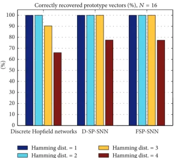
Discrete Hopfield networks D-SP-SNN FSP-SNN 0 10 20 30 40 50 60 70 80 90 100 (%) Hamming dist.= 2 Hamming dist.= 3 Hamming dist.= 1 Hamming dist.= 4

Correctly recovered prototype vectors (%),𝑁 = 16

Figure 2: The figure shows the percentage of correctly recovered desired patterns for all possible initial conditions inExample 8for the proposed D-SP-SNN and its 1-bit version FSP-SNN as compared to traditional Hopfield network (16-neuron case).

Hopfield network for 1 and 2 Hamming distance cases while the all the networks perform poorly (less than 20%) at 3-Hamming distance case.

Example 8. The desired prototype vectors are

D =[[_[ [ 1 1 1 1 1 1 1 1 −1 −1 −1 −1 −1 −1 −1 −1 1 1 1 1 −1 −1 −1 −1 1 1 1 1 −1 −1 −1 −1 1 1 −1 −1 1 1 −1 −1 1 1 −1 −1 1 1 −1 −1 1 −1 1 −1 1 −1 1 −1 1 −1 1 −1 1 −1 1 −1 ] ] ] ] . (41)

The weight matrices A and W and threshold vector b are obtained as follows by using the outer-product-based design (Hebb-learning [19]) inAppendix B: A = 4I, W = [ [ [ [ [ [ [ [ [ [ [ [ [ [ [ [ [ [ 0 2 2 0 2 0 0 −2 2 0 0 −2 0 −2 −2 −4 2 0 0 2 0 2 −2 0 0 2 −2 0 −2 0 −4 −2 2 0 0 2 0 −2 2 0 0 −2 2 0 −2 −4 0 −2 0 2 2 0 −2 0 0 2 −2 0 0 2 −4 −2 −2 0 2 0 0 −2 0 2 2 0 0 −2 −2 −4 2 0 0 −2 0 2 −2 0 2 0 0 2 −2 0 −4 −2 0 2 −2 0 0 −2 2 0 2 0 0 2 −2 −4 0 −2 0 −2 2 0 −2 0 0 2 0 2 2 0 −4 −2 −2 0 −2 0 0 2 2 0 0 −2 0 −2 −2 −4 0 2 2 0 2 0 0 −2 0 2 −2 0 −2 0 −4 −2 2 0 0 2 0 2 −2 0 0 −2 2 0 −2 −4 0 −2 2 0 0 2 0 −2 2 0 −2 0 0 2 −4 −2 −2 0 0 2 2 0 −2 0 0 2 0 −2 −2 −4 2 0 0 −2 2 0 0 −2 0 2 2 0 −2 0 −4 −2 0 2 −2 0 0 2 −2 0 2 0 0 2 −2 −4 0 −2 0 −2 2 0 0 −2 2 0 2 0 0 2 −4 −2 −2 0 −2 0 0 2 −2 0 0 2 0 2 2 0 ] ] ] ] ] ] ] ] ] ] ] ] ] ] ] ] ] ] , b = 0. (42)

Figure 2 shows the percentage of correctly recovered desired patterns for all possible initial conditions x(𝑘) ∈ (−1, +1)16_{, in the proposed D-SP-SNN and FSP-SNN as} compared to discrete Hopfield network.

The total number of different possible combinations for the initial conditions for this example is 64, 480, 2240

and 7280 for 1-, 2-, 3-, and 4-Hamming distance cases, respectively, which could be calculated by 𝑚_𝑑 × 𝐶(16, 𝐾), where𝑚_𝑑= 4 and 𝐾 = 1, 2, 3, and 4.

As seen fromFigure 2the performance of the proposed networks D-SP-SNN and FSP-SNN is the same as that of discrete Hopfield Network for 1-Hamming and 2-Hamming

(7)

States for D-SP-SNN States for D-SP-SNN 5 0 −5 5 0 −5 5 0 −5 3 2 1 3 2 1 3 2 1 3 2 1 4 2 0 0 100 200 300 400 𝑥1 (𝑘 ) 𝑥2 (𝑘 𝑘 0 100 200 300 400 𝑘 0 100 200 300 400 𝑘 0 100 200 300 400 𝑘 0 100 200𝑘 300 400 0 100 200 300 400 𝑘 0 100 200 300 400 𝑘 0 100 200 300 400 𝑘 ) 𝑥3 (𝑘 ) 𝑥4 (𝑘 ) 𝑥5 (𝑘 ) 𝑥6 (𝑘 ) 𝑥7 (𝑘 ) 𝑥8 (𝑘 ) (a) States for D-SP-SNN States for D-SP-SNN 𝑥9 (𝑘 ) 𝑥10 (𝑘 ) 𝑥11 (𝑘 ) 𝑥12 (𝑘 ) 𝑥13 (𝑘 ) 𝑥14 (𝑘 ) 𝑥15 (𝑘 ) 𝑥16 (𝑘 ) −1 −2 −3 −1 −2 −3 0 −2 −4 0 −2 −4 −1 −2 −3 −1 −2 −3 0 −2 −4 0 −2 −4 0 100 200 300 400 𝑘 0 100 200 300 400 𝑘 0 100 200 300 400 𝑘 0 100 200 300 400 𝑘 0 100 200𝑘 300 400 0 100 200 300 400 𝑘 0 100 200 300 400 𝑘 0 100 200 300 400 𝑘 (b)

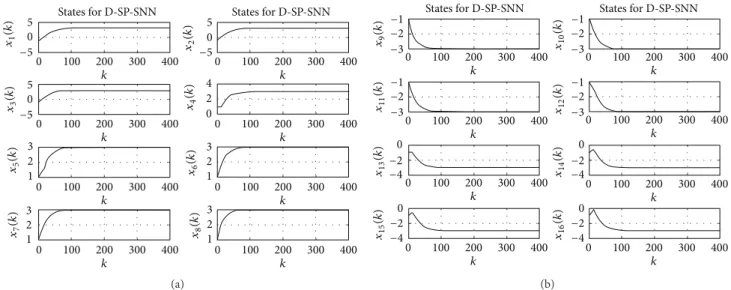
Figure 3: Typical plot for evolutions of states (a) 1 to 8 and (b) 9 to 16 inExample 8by the D-SP-SNN.

2 2 0 −2 1 0 −1 1 0 1 0 1 0 −1 1 0.5 1 0.5 0.5 1 0 0.5 0 0 100 200 300 400 𝑘 0 100 200 300 400 𝑘 0 100 200 300 400 𝑘 0 100 200 300 400 𝑘 0 100 200 300 400 𝑘 0 100 200 300 400 𝑘 0 100 200 300 400 𝑘 0 100 200 300 400 𝑘

SINR(𝑘) for D-SP-SNN SINR(𝑘) for D-SP-SNN

PS1 (𝑘 ) PS2 (𝑘 ) PS3 (𝑘 ) PS4 (𝑘 ) PS 5 (𝑘 ) PS 6 (𝑘 ) PS7 (𝑘 ) PS8 (𝑘 ) (a) 1 0.5 0 1 0.5 0 1 0.5 1 0.5 0 2 1 0 100 0 −100 100 0 −100 −5 0 5 0 100 200 300 400 𝑘 0 100 200 300 400 𝑘 0 100 200 300 400 𝑘 0 100 200 300 400 𝑘 0 100 200 300 400 𝑘 0 100 200 300 400 𝑘 0 100 200 300 400 𝑘 0 100 200 300 400 𝑘

PS 9 (𝑘 ) PS 10 (𝑘 ) PS11 (𝑘 ) PS12 (𝑘 ) PS 13 (𝑘 ) PS 14 (𝑘 ) PS15 (𝑘 ) PS16 (𝑘 ) (b)

Figure 4: Evolutions of pseudo-SINRs for the states inFigure 3inExample 8by the D-SP-SNN. (a) Pseudo-SINRs 1 to 8 and (b) pseudo-SINRs 9 to 16.

distance cases (%100 for all networks). However, the D-SP-SNN and FSP-D-SP-SNN give better performance than the discrete Hopfield network does for 3- and 4- Hamming distance cases. Typical plots for evolution of states in Example 8 by the D-SP-SNN are shown in Figure 3. The evolution of corresponding pseudo-SINRs is given byFigure 4. The figure shows that the pseudo-SINRs approach to constant value 1 as states converge to the equilibrium point.

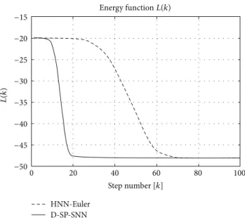
Evolutions of the Lyapunov function in (37) for the states of Figure 3in Example 8 are given in Figure 5. The figure shows that the proposed D-SP-SNN minimizes the Lyapunov function of Hopfield neural network with the same weight matrix.

Example 9. In Examples 7 and 8, the desired vectors are

orthogonal. In this example, the desired vectors represent

numbers 1, 2, 3, and 4, which are not orthogonal to each other. The numbers are represented by 25 neurons. The weight matrix is determined by the Hebb learning as in the previous examples. In the rest of the examples in this paper, we set 𝜎₁ = 1, 𝜅₁ = 10, 𝜎₂ = 10, 𝜅₂ = 1, and 𝛼(𝑘) = 0.01, for all 𝑘.

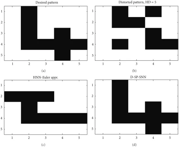
Figure 6 shows desired pattern 1, a distorted pattern 1 where the Hamming Distance (HD) is 5, the result of HNN-Euler, and the result of the D-SP-SNN using the distorted pattern as initial condition. As seen from the figure, the proposed D-SP-SNN succeeds to recover the number while the HNN-Euler fails for the same parameters and weight matrix.

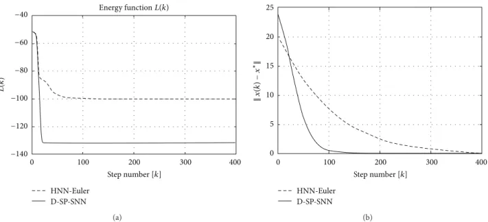
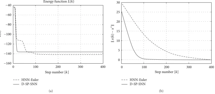
The evolutions of the Lyapunov function in (37) and the norm of the difference between the state vector and equilibrium point for pattern 1 in Figure 6 are shown in Figure 7. As seen from the figure, (i) the proposed D-SP-SNN

(8)

−15 −20 −25 −30 −35 −40 −45 −50 0 20 40 60 80 100 Step number [𝑘] 𝐿( 𝑘) Energy function𝐿(𝑘) HNN-Euler D-SP-SNN

Figure 5: Evolution of Lyapunov function in (37) inExample 8(𝑁 = 16).

1 2 3 4 5 1 2 3 4 5 Desired pattern (a) 1 2 3 4 5 1 2 3 4 5 Distorted pattern, HD= 5 (b) 1 2 3 4 5 1 2 3 4 5 HNN-Euler Appr. (c) 1 2 3 4 5 1 2 3 4 5 D-SP-SNN (d)

(9)

−40 −60 −80 −100 −120 −140 𝐿( 𝑘) Step number [_𝑘] 0 100 200 300 400 Energy function𝐿(𝑘) HNN-Euler D-SP-SNN (a) Step number [_𝑘] 0 100 200 300 400 HNN-Euler D-SP-SNN 25 20 15 10 5 0 ‖𝑥 (𝑘 )− 𝑥 ∗‖ (b)

Figure 7: Evolution of (a) Lyapunov function in (37) and (b) norm of the difference between the state vector and equilibrium point in

Example 9for pattern 1 (𝑁 = 25).

1 2 3 4 5 1 2 3 4 5 Desired pattern (a) 1 2 3 4 5 1 2 3 4 5 Distorted pattern, HD_{= 5} (b) 1 2 3 4 5 1 2 3 4 5 HNN-Euler appr. (c) 1 2 3 4 5 1 2 3 4 5 D-SP-SNN (d)

Figure 8: (a) Desired pattern 2, (b) distorted pattern 2 (HD = 5), (c) result of HNN-Euler, and (d) Result of D-SP-SNN inExample 9.

minimizes the Lyapunov function of Hopfield neural net-work, and (ii) the proposed D-SP-SNN converges faster than its HNN-Euler counterpart with the same weight matrix for this example.

Figure 8 shows desired pattern 2, a distorted pattern 2 where the HD is 5, the result of HNN-Euler, and the result of D-SP-SNN using the distorted pattern as initial condition. As seen from the figure, the proposed D-SP-SNN succeeds to

(10)

0 −2 −4 0 −5 −10 0 −5 5 5 10 0 0 −20 2 2 1 −10 0 −2 −4 0 100 200 300 400 𝑥1 (𝑘 ) 𝑥2 (𝑘 𝑘 0 100 200 300 400 𝑘 0 100 200 300 400 𝑘 0 100 200 300 400 𝑘 0 100 200 300 400 𝑘 0 0 4 0 100 200 300 400 𝑘 0 100 200 300 400 𝑘 0 100 200 300 400 𝑘 ) 𝑥3 (𝑘 ) 𝑥5 (𝑘 ) 𝑥7 (𝑘 ) 𝑥4 (𝑘 ) 𝑥6 (𝑘 ) 𝑥8 (𝑘 )

States for HNN-Euler approx. States for HNN-Euler approx.

(a)

0 100 200 300 400

−4

−20

𝑘

0 100 200 300 400 −4 −2 0 𝑘 0 100 200 300 400 −4 −2 0 𝑘 0 100 200 300 400 0 0.5 1 𝑘 0 100 200 300 400 −10 −5 0 𝑘 0 100 200 300 400 −4 −2 0 𝑘 0 100 200 300 400 −5 0 5 𝑘 0 100 200 300 400 −4 −2 0 𝑘 𝑥9 (𝑘 ) 𝑥10 (𝑘 ) 𝑥11 (𝑘 ) 𝑥12 (𝑘 ) 𝑥13 (𝑘 ) 𝑥14 (𝑘 ) 𝑥15 (𝑘 ) 𝑥16 (𝑘 ) (b) 0 100 200 300 400 𝑘 0 100 200 300 400 𝑘 0 100 200 300 400 𝑘 0 100 200 300 400 𝑘 0 100 200𝑘 300 400 0 100 200 300 400 𝑘 0 100 200 300 400 𝑘 0 100 200 300 400 𝑘

𝑥17 (𝑘 ) 𝑥18 (𝑘 ) 𝑥19 (𝑘 ) 𝑥20 (𝑘 ) 𝑥21 (𝑘 ) 𝑥22 (𝑘 ) 𝑥23 (𝑘 ) 𝑥24 (𝑘 ) 10 5 0 10 5 0 20 0 −20 20 0 −20 2 1.5 1 0 0 −2 −4 0 −2 −5 −10 −4 (c)

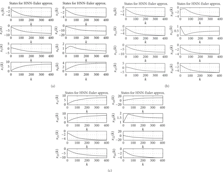
Figure 9: Evolutions of states (a) 1 to 8, (b) 9 to 16, and (c) 17 to 24 inExample 9for pattern 2 by HNN-Euler.

recover the number while the HNN-Euler fails for the same parameters and weight matrix.

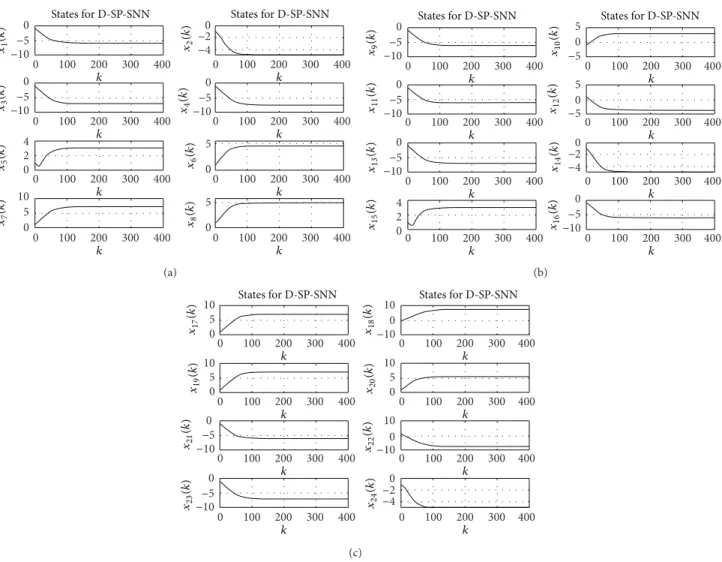
Evolutions of states inExample 9for pattern 2 by HNN-Euler and by D-SP-SNN are shown in Figures 9 and 10, respectively. The figures show that the states of proposed D-SP-SNN converge faster than those of its HNN-Euler counterpart for the same parameter settings.

Figure 11shows the evolutions of pseudo-SINRs of states inExample 9for pattern 2 by D-SP-SNN. The figure shows that the pseudo-SINRs approach to constant value 1 as states converge to the equilibrium point.

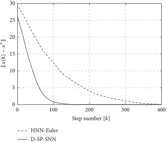
The evolutions of the norm of the difference between the state vector and equilibrium point for pattern 2 in Figure 8are shown inFigure 12. As seen from the figure, the proposed D-SP-SNN converges much faster than its HNN-Euler counterpart.

Figure 13shows desired pattern 3, a distorted pattern 3 where the HD is 5, the result of HNN-Euler, and the result of the D-SP-SNN using the distorted pattern as initial condition. As seen from the figure, the proposed D-SP-SNN succeeds to recover the number while its HNN-Euler counterpart fails for the same parameters and weight matrix.

The evolutions of the Lyapunov function and the norm of the difference between the state vector and equilibrium point for pattern 3 inFigure 13are shown in Figure 14. As seen from the figure, (i) the proposed D-SP-SNN minimizes the Lyapunov function of Hopfield neural network, and (ii) the proposed D-SP-SNN converges faster than its HNN-Euler counterpart with the same weight matrix for this example.

Figure 15shows desired pattern 4, a distorted pattern 4 where the HD is 5, the result of HNN-Euler, and the result of the D-SP-SNN using the distorted pattern as initial condition. As seen from the figure, the proposed D-SP-SNN succeeds to recover the number while its HNN-Euler counterpart fails for the same parameters settings.

The evolutions of the Lyapunov function and the norm of the difference between the state vector and equilibrium point for pattern 4 inFigure 15are shown inFigure 16. As seen from the figure, (i) the proposed D-SP-SNN minimizes the Lyapunov function of Hopfield Neural Network, and (ii) the proposed D-SP-SNN converges faster than its HNN-Euler counterpart with the same weight matrix for this example.

Example 10. In this and in the following example, we examine

(11)

𝑥1 (𝑘 ) 𝑥2 (𝑘 ) 𝑥3 (𝑘 ) 𝑥5 (𝑘 ) 𝑥7 (𝑘 ) 𝑥4 (𝑘 ) 𝑥6 (𝑘 ) 𝑥8 (𝑘 ) 0 100 200 300 400 𝑘 0 100 200 300 400 𝑘 0 100 200 300 400 𝑘 0 100 200 300 400 𝑘 0 100 200 300 400 𝑘 0 100 200 300 400 𝑘 0 100 200 300 400 𝑘 0 100 200 300 400 𝑘 −10 −5 0 −4 −20 −−10 5 0 −−10 5 0 0 0 0 5 10 2 4 5 0 5

States for D-SP-SNN States for D-SP-SNN

(a) 𝑥9 (𝑘 ) 𝑥10 (𝑘 ) 𝑥11 (𝑘 ) 𝑥12 (𝑘 ) 𝑥13 (𝑘 ) 𝑥14 (𝑘 ) 𝑥15 (𝑘 ) 𝑥16 (𝑘 ) 0 100 200 300 400 𝑘 0 100 200 300 400 𝑘 0 100 200 300 400 𝑘 0 100 200 300 400 𝑘 0 100 200𝑘 300 400 0 100 200 300 400 𝑘 0 100 200 300 400 𝑘 0 100 200 300 400 𝑘 −−10 5 0 −−10 5 0 −10 −5 0 −−10 5 0 −4 −2 −5 0 0 5 −5 0 5 0 2 4

States for D-SP-SNN States for D-SP-SNN

(b) 0 100 200 300 400 𝑘 0 100 200 300 400 𝑘 0 100 200 300 400 𝑘 0 100 200 300 400 𝑘 0 100 200𝑘 300 400 0 100 200 300 400 𝑘 0 100 200 300 400 𝑘 0 100 200 300 400 𝑘 𝑥17 (𝑘 ) 𝑥18 (𝑘 ) 𝑥19 (𝑘 ) 𝑥20 (𝑘 ) 𝑥21 (𝑘 ) 𝑥22 (𝑘 ) 𝑥23 (𝑘 ) 𝑥24 (𝑘 ) −4 −2 0 −−10 5 0 0 −10 −10 −5 0 0 5 10 0 5 10 0 5 10 10 0 −10 10 States for D-SP-SNN States for D-SP-SNN (c)

Figure 10: Evolutions of states (a) 1 to 8, (b) 9 to 16, and (c) 17 to 24 inExample 9for pattern 2 by D-SP-SNN.

problem. Clustering is used in a wide range of applica-tions, such as engineering, biology, marketing, information retrieval, social network analysis, image processing, text min-ing, finding communities, influencers, and leaders in online or offline social networks. Data clustering is a technique that enables dividing large amounts of data into groups/clusters in an unsupervised manner such that the data points in the same group/cluster are similar and those in different clusters are dissimilar according to some defined similarity criteria. The clustering problem is an NP-complete, and its general solution even for 2-clustering case is not known. It is well known that the clustering problem can be formulated in the form of the Lyapunov function of the HNN. The weight matrix is chosen as the distance matrix of the dataset and is the same for both HNN-Euler and D-SP-SNN.

In what follows, we compare the performance of the pro-posed D-SP-SNN as compared to its HNN-Euler counterpart as applied to clustering problems for the very same parameter settings. Two-dimensional 16 data points to be bisected are shown inFigure 17. The clustering results are also shown in Figure 17. As seen from the figure, the D-SP-SNN finds the

optimum solution for this toy example. HNN-Euler also gives the same solution.

The evolutions of states in the clustering by HNN-Euler and by D-SP-SNN are shown in Figures 18 and 19, respectively. As seen from the figures, the states of the proposed D-SP-SNN converge faster that those of its HNN-Euler counterpart.

The evolutions of psuedo-SINRs of states in the clustering by D-SP-SNN inExample 10(𝑁 = 16) are given byFigure 20. The figure shows that the pseudo-SINRs approach to constant value 1 as states converge to the equilibrium point.

The evolutions of Lyapunov function and the norm of the difference between the state vector and equilibrium point in Example 10are given inFigure 21. The figure confirms that (i) the proposed D-SP-SNN minimizes the Lyapunov function of Hopfield neural network and (ii) the proposed D-SP-SNN converges faster than its HNN-Euler counterpart with the same weight matrix.

Example 11. In this example, there are 40 data points as shown

inFigure 22. The figure also shows the bisecting clustering results by𝑘-means algorithm and the proposed D-SP-SNN.

(12)

PS1 (𝑘 ) PS2 (𝑘 ) PS3 (𝑘 ) PS4 (𝑘 ) PS 5 (𝑘 ) PS6 (𝑘 ) PS 7 (𝑘 ) PS 8 (𝑘 ) 1 0.5 0 1 0.5 0 1 0.5 0 1 0.5 0 1 0.5 0 1 0.5 0 1 0.5 0 50 0 −50 0 100 200 300 400 𝑘 0 100 200 300 400 𝑘 0 100 200 300 400 𝑘 0 100 200 300 400 𝑘 0 100 200𝑘 300 400 0 100 200 300 400 𝑘 0 100 200 300 400 𝑘 0 100 200 300 400 𝑘

Pseudo-SINR(𝑘) for D-SP-SNN Pseudo-SINR(𝑘) for D-SP-SNN

(a) PS 9 (𝑘 ) PS 10 (𝑘 ) PS11 (𝑘 ) PS 12 (𝑘 ) PS13 (𝑘 ) PS 14 (𝑘 ) PS15 (𝑘 ) PS16 (𝑘 ) 1 0.5 0 1 0.5 0 1 0.5 0 1 1 0.5 0 0 1 0.5 50 100 0 0 −1 1 0 −1 0 100 200 300 400 𝑘 0 100 200 300 400 𝑘 0 100 200 300 400 𝑘 0 100 200 300 400 𝑘 0 100 200𝑘 300 400 0 100 200 300 400 𝑘 0 100 200 300 400 𝑘 0 100 200 300 400 𝑘

Pseudo-SINR(_{𝑘) for D-SP-SNN} Pseudo-SINR(_{𝑘) for D-SP-SNN}

(b) PS17 (𝑘 ) PS18 (𝑘 ) PS 19 (𝑘 ) PS 20 (𝑘 ) PS 21 (𝑘 ) PS22 (𝑘 ) PS23 (𝑘 ) PS24 (𝑘 ) 1 0.5 0 1 0.5 0 1 0.5 0 1 0.5 0 1 0.5 0 1 0.5 0 1 0 −1 1 0 −1 0 100 200 300 400 𝑘 0 100 200 300 400 𝑘 0 100 200 300 400 𝑘 0 100 200 300 400 𝑘 0 100 200𝑘 300 400 0 100 200 300 400 𝑘 0 100 200 300 400 𝑘 0 100 200 300 400 𝑘

Pseudo-SINR(_{𝑘) for D-SP-SNN} Pseudo-SINR(_{𝑘) for D-SP-SNN}

(c)

Figure 11: Evolutions of pseudo-SINRs of states (a) 1 to 8, (b) 9 to 16, and (c) 17 to 24 inExample 9for pattern 2 by D-SP-SNN.

25 30 20 15 10 5 0 ‖𝑥 (𝑘 )− 𝑥 ∗ ‖ Step number [_𝑘] HNN-Euler D-SP-SNN 0 100 200 300 400

(13)

1 2 3 4 5 1 2 3 4 5 Desired pattern (a) 1 2 3 4 5 1 2 3 4 5 Distorted pattern, HD_{= 5} (b) 1 2 3 4 5 1 2 3 4 5 HNN-Euler appr. (c) 1 2 3 4 5 1 2 3 4 5 D-SP-SNN (d)

Figure 13: (a) Desired pattern 3, (b) distorted pattern 3 (HD = 5), (c) result of HNN-Euler, and (d) result of D-SP-SNN inExample 9.

−40 −80 −100 −120 −140 −60 −160 𝐿( 𝑘) 0 100 200 300 400 Step number [𝑘] Energy function𝐿(𝑘) HNN-Euler D-SP-SNN (a) 0 100 200 300 400 Step number [𝑘] HNN-Euler D-SP-SNN 30 25 20 15 10 5 0 ‖𝑥 (𝑘 )− 𝑥 ∗‖ (b)

Figure 14: Evolution of (a) Lyapunov function and (b) norm of the difference between the state vector and equilibrium point inExample 9 for pattern 3 (𝑁 = 25).

(14)

1 2 3 4 5 1 2 3 4 5 Desired pattern (a) 1 2 3 4 5 1 2 3 4 5 Distorted pattern, HD= 5 (b) 1 2 3 4 5 1 2 3 4 5 HNN-Euler appr. (c) 1 2 3 4 5 1 2 3 4 5 D-SP-SNN (d)

Figure 15: (a) Desired pattern 4, (b) distorted pattern 4 (HD = 5), (c) result of HNN-Euler, and (d) result of D-SP-SNN inExample 9.

−40 −80 −100 −120 −140 −60 −160 𝐿( 𝑘) 0 100 200 300 400 Step number [𝑘] Energy function𝐿(𝑘) HNN-Euler D-SP-SNN (a) ‖ 𝑥(𝑘 )− 𝑥 ∗‖ 0 100 200 300 400 Step number [𝑘] HNN-Euler D-SP-SNN 30 25 20 15 10 5 0 (b)

Figure 16: Evolutions of (a) Lyapunov function and (b) norm of the difference between the state vector and equilibrium point inExample 9 for pattern 4 (𝑁 = 25).

(15)

−100 0 100 200 300 400 500 600 700 800 900 −150 −100 −50 0 50 100 150 200 250 300 1 2 3 4 5 6 7 8 9 10 11 12 13 14 15 16 Clustering result-D-SP-SNN 𝑦 -co o rdina te (m) 𝑥-coordinate (m)

Figure 17: Result of clustering by D-SP-SNN,𝑁 = 16 inExample 10.

5 0 5 0 −5 5 0 0.5 0 −5 4 2 0 4 2 0 4 2 0 1 1 0 −1 0 100 200 300 400 0 100 200 300 400 𝑘 𝑘 0 100 200 300 400 𝑘 0 100 200 300 400 𝑘 0 100 200𝑘 300 400 0 100 200 300 400 𝑘 0 100 200 300 400 𝑘 0 100 200 300 400 𝑘 𝑥1 (𝑘 ) 𝑥2 (𝑘 ) 𝑥3 (𝑘 ) 𝑥4 (𝑘 ) 𝑥5 (𝑘 ) 𝑥6 (𝑘 ) 𝑥7 (𝑘 ) 𝑥8 (𝑘 )

(a) 5 0 −5 5 0 −5 1 0 −1 1 0 −1 0 0 −2 −4 0 −2 −4 0 −2 −4 −2 −4 0 100 200 300 400 𝑘 0 100 200 300 400 𝑘 0 100 200 300 400 𝑘 0 100 200 300 400 𝑘 0 100 200𝑘 300 400 0 100 200 300 400 𝑘 0 100 200 300 400 𝑘 0 100 200 300 400 𝑘 𝑥9 (𝑘 ) 𝑥10 (𝑘 ) 𝑥11 (𝑘 ) 𝑥12 (𝑘 ) 𝑥13 (𝑘 ) 𝑥14 (𝑘 ) 𝑥15 (𝑘 ) 𝑥16 (𝑘 )

(b)

Figure 18: Evolutions of states (a) 1 to 8 and (b) 9 to 16 in the clustering by HNN-Euler inExample 10(𝑁 = 16).

States for D-SP-SNN States for D-SP-SNN 5 0 5 0 −5 5 0 1 0 −5 4 2 0 4 2 0 4 2 0 2 2 0 −2 0 100 200 300 400 0 100 200 300 400 𝑘 𝑘 0 100 200 300 400 𝑘 0 100 200 300 400 𝑘 0 100 200𝑘 300 400 0 100 200 300 400 𝑘 0 100 200 300 400 𝑘 0 100 200 300 400 𝑘 𝑥1 (𝑘 ) 𝑥2 (𝑘 ) 𝑥3 (𝑘 ) 𝑥4 (𝑘 ) 𝑥5 (𝑘 ) 𝑥6 (𝑘 ) 𝑥7 (𝑘 ) 𝑥8 (𝑘 ) (a) 0 5 0 −5 5 0 −5 2 0 −2 2 0 −2 0 0 −2 −4 −2 −4 0 −2 −4 −2 −4 0 100 200 300 400 𝑘 0 100 200 300 400 𝑘 0 100 200 300 400 𝑘 0 100 200 300 400 𝑘 0 100 200𝑘 300 400 0 100 200 300 400 𝑘 0 100 200 300 400 𝑘 0 100 200 300 400 𝑘 𝑥9 (𝑘 ) 𝑥10 (𝑘 ) 𝑥11 (𝑘 ) 𝑥12 (𝑘 ) 𝑥13 (𝑘 ) 𝑥14 (𝑘 ) 𝑥15 (𝑘 ) 𝑥16 (𝑘 ) States for D-SP-SNN States for D-SP-SNN (b)

(16)

0 100 200 300 400 𝑘 0 100 200 300 400 𝑘 0 100 200 300 400 𝑘 0 100 200 300 400 𝑘 0 100 200 300 400 𝑘 0 100 200 300 400 𝑘 0 100 200 300 400 𝑘 0 100 200 300 400 𝑘 2 1 0 2 1 0 2 1 0 2 0 −2 2 0 −2 2 0 −2 1 0 −1 2 1 0 −1 PS1 (𝑘 ) PS 2 (𝑘 ) PS3 (𝑘 ) PS 4 (𝑘 ) PS5 (𝑘 ) PS6 (𝑘 ) PS7 (𝑘 ) PS8 (𝑘 )

(a) 0 100 200 300 400 𝑘 0 100 200 300 400 𝑘 0 100 200 300 400 𝑘 0 100 200 300 400 𝑘 0 100 200 300 400 𝑘 0 100 200 300 400 𝑘 0 100 200 300 400 𝑘 0 100 200 300 400 𝑘 0.51 0 0.51 0 0.5 1 0 0.51 0 2 0 −2 2 0 −2 1 0 −1 1 0 −1 PS9 (𝑘 ) PS10 (𝑘 ) PS11 (𝑘 ) PS12 (𝑘 ) PS 13 (𝑘 ) PS14 (𝑘 ) PS 15 (𝑘 ) PS 16 (𝑘 )

SINR (𝑘) for D-SP-SNN SINR (𝑘) for D-SP-SNN

(b)

Figure 20: Evolutions of psuedo-SINRs of states (a) 1 to 8 and (b) 9 to 16 in the clustering by D-SP-SNN inExample 10(𝑁 = 16).

0 20 40 60 80 0 −10 −20 −30 −40 −50 𝐿( 𝑘) Step number [𝑘] HNN-Euler D-SP-SNN Energy function𝐿(𝑘) (a) 14 12 10 8 6 4 2 0 0 100 200 300 400 Step number [𝑘] HNN-Euler D-SP-SNN ‖𝑥 (𝑘 )− 𝑥 ∗‖ (b)

Figure 21: Evolution of (a) Lyapunov function and (b) norm of the difference between the state vector and equilibrium point inExample 10 (𝑁 = 16). 38 30 22 14 6 5 13 21 29 37 4 12 20 28 36 39 31 23 15 7 8 16 24 32 40 1 9 17 25 33 2 10 18 26 34 3 11 19 27 35 500 400 300 200 100 0 −100 −200 −300 −400 −500 500 600 400 300 200 100 0 −100 −200 −300 −400 −500 𝑦 -co o rdina te (m) 𝑥-coordinate (m)

Clustering result-𝑘-means

(a) 38 30 22 14 6 39 31 23 15 7 8 16 24 32 40 1 9 17 25 33 37 29 21 13 5 4 12 20 28 36 3 2 11 19 27 35 10 18 26 34 500 400 300 200 100 0 −100 −200 −300 −400 −500 500 600 400 300 200 100 0 −100 −200 −300 −400 −500 𝑦 -co o rdina te (m) 𝑥-coordinate (m) Clustering result-D-SP-SNN (b)

(17)

PS1 (𝑘 ) PS2 (𝑘 ) PS 3 (𝑘 ) PS 4 (𝑘 ) PS 5 (𝑘 ) PS6 (𝑘 ) PS 7 (𝑘 ) PS 8 (𝑘 ) 2 0 −2 2 0 −2 2 0 −2 2 0 −2 1 0.5 0 1 0.5 0 1 0 −1 1 0 −1 0 100 200 300 400 𝑘 0 100 200 300 400 𝑘 0 100 200 300 400 𝑘 0 100 200 300 400 𝑘 0 100 200𝑘 300 400 0 100 200 300 400 𝑘 0 100 200 300 400 𝑘 0 100 200 300 400 𝑘 SINR(𝑘) for D-SP-SNN SINR(𝑘) for D-SP-SNN

Figure 23: Evolution of pseudo-SINRs of states 1 to 8 inExample 11by the D-SP-SNN, (𝑁 = 40).

0 10 20 30 40 50 60 0 −50 −100 −150 𝐿( 𝑘) Step number [𝑘] Energy function𝐿(𝑘) HNN-Euler D-SP-SNN (a) 25 20 15 10 5 0 0 50 100 150 200 250 300 350 400 Step number [_𝑘] HNN-Euler D-SP-SNN ‖𝑥 (𝑘 )− 𝑥 ∗‖ (b)

Figure 24: Evolution of (a) Lyapunov function and (b) norm of the difference between the state vector and equilibrium point inExample 11 (𝑁 = 40).

As seen from the figure, while 𝑘-means fail to find the optimum clustering solution for this example (for a randomly given initial values), the proposed D-SP-SNN succeeds in finding the optimum solution (for the same initial values).

Figure 23shows the evolution of pseudo-SINRs of states by the D-SP-SNN. The figure shows that the pseudo-SINRs approach to constant value 1 as states converge to the equilibrium point, as before.

Evolutions of the Lyapunov function and the norm of the difference between the state vector and equilibrium point are shown in Figure 24. The figure confirms the superior convergence speed of the D-SP-SNN as compared to its HNN-Euler counterpart.

4. Conclusions

In this paper, we present and analyze a discrete recurrent non-linear system which includes the Hopfield neural networks [1,2] and the nonlinear sigmoid power control algorithm for cellular radio systems in [13], as special cases by properly

choosing the functions. This paper extends the results in [11], which are for autonomous linear systems, to nonlinear case. The proposed system can be viewed as a discrete-time realization of a recently proposed continuous-time network in [12]. In this paper, we focus on discrete-time analysis and present various novel key results concerning the discrete-time dynamics of the proposed system, some of which are as follows: (i) the proposed network is shown to be stable in synchronous and asynchronous work mode in discrete time; (ii) a novel concept called Pseudo-SINR (pseudo-signal-to-interference-noise ratio) is introduced for discrete-time nonlinear systems; (iii) it is shown that when the network approaches one of its equilibrium points, the instantaneous Pseudo-SINRs become equal to a constant target value.

The simulation results confirm the novel results (e.g., Pseudo-SINR convergence, etc.) presented and show a supe-rior performance of the proposed network as compared to its Hopfield network counterpart in various associative memory systems and clustering examples. Moreover, the results show that the proposed network minimizes the Lyapunov function

(18)

of the Hopfield neural networks. The disadvantage of the D-SP-SNN is that it increases the computational burden.

Appendices

A. Lipschitz Constant of the Sigmoid Function

In what follows, we will show the sigmoid function (𝑓(𝑎) = 1 − (2/(1 + exp(−𝜎𝑎))), 𝜎 > 0) that has the global Lipschitz constant𝑘 = 0.5𝜎. Since 𝑓(⋅) is a differentiable function, we can apply the mean value theorem:

𝑓 (𝑎) − 𝑓 (𝑏) = (𝑎 − 𝑏) 𝑓󸀠(𝜇𝑎 + (1 − 𝜇) (𝑏 − 𝑎))

with𝜇 ∈ [0, 1] . (A.1) The derivative of𝑓(⋅) is 𝑓󸀠(𝑎) = −2𝜎/𝑒𝜎𝑎(1+𝑒−𝜎𝑎)2whose maximum is at the point𝑎 = 0; that is, |𝑓󸀠(𝑎)| ≤ 0.5𝜎. So we obtain the following inequality:

󵄨󵄨󵄨󵄨𝑓(𝑎) − 𝑓(𝑏)󵄨󵄨󵄨󵄨 ≤ 𝑘|𝑎 − 𝑏|, (A.2) where𝑘 = 0.5𝜎 is the global Lipschitz constant of the sigmoid function.

B. Outer Product-Based Network Design

Let us assume that𝐿 desired prototype vectors are orthogonal and each element of a prototype vector is either−1 or +1.

Step 1. Calculate the sum of outer products of the prototype

vectors (Hebb Rule, [19]) Q = 𝐿 ∑ 𝑠=1d𝑠d 𝑇 𝑠. (B.1)

Step 2. Determine the diagonal matrix A and W as follows:

𝑎_𝑖𝑗= {𝑞𝑖𝑖+ 𝜌 if 𝑖 = 𝑗,

0 if𝑖 ̸= 𝑗, 𝑖, 𝑗 = 1, . . . , 𝑁, (B.2) where𝜌 is a real number and

𝑤_𝑖𝑗= {0_𝑞 if𝑖 = 𝑗,

𝑖𝑗 if𝑖 ̸= 𝑗, 𝑖, 𝑗 = 1, . . . , 𝑁, (B.3) where𝑞_𝑖𝑗shows the entries of matrix Q, 𝑁 is the dimension of the vector x, and 𝐿 is the number of the prototype vectors (𝑁 > 𝐿 > 0). In (B.2), 𝑞_𝑖𝑖 = 𝐿 from (B.1) since {d_𝑠} is from (−1, +1)𝑁. It is observed that 𝜌 = 0 gives relatively good performance; however, by examining the nonlinear state equations inSection 2, it can be seen that the proposed networks D-SP-SNN and FSP-SNN contain the prototype vectors at their equilibrium points for a relatively large interval of𝜌.

Another choice of 𝜌 in (B.2) is 𝜌 = 𝑁 − 2𝐿 which yields𝑎_𝑖𝑖 = 𝑁 − 𝐿. In what follows we show that this choice

also assures that{d_𝑗}𝐿_𝑗=1 are the equilibrium points of the networks. From (B.1)–(B.3) [−A + W] = − (𝑁 − 𝐿) I +∑𝐿 𝑠=1d𝑠d 𝑇 𝑠 − 𝐿I, (B.4) where I represents the identity matrix. Since d_𝑠∈ (−1, +1)𝑁, then||d_𝑠||2₂= 𝑁. Using (B.4) and the orthogonality properties of the set{d_𝑠}𝐿_𝑠=1gives the following:

[−A + W] d𝑠= − (𝑁 − 𝐿) d𝑠+ (𝑁 − 𝐿) d𝑠= 0. (B.5) So, the prototype vectors{d_𝑗}𝐿_𝑗=1correspond to equilib-rium points.

References

[1] J. J. Hopfield, “Neural networks and physical systems with emergent collective computational abilities,” Proceedings of the

National Academy of Sciences of the United States of America,

vol. 79, no. 8, pp. 2554–2558, 1982.

[2] J. J. Hopfield and D. W. Tank, “‘Neural’ computation of decisons in optimization problems,” Biological Cybernetics, vol. 52, no. 3, pp. 141–152, 1985.

[3] S. Matsuda, “Optimal Hopfield network for combinatorial optimization with linear cost function,” IEEE Transactions on

Neural Networks, vol. 9, no. 6, pp. 1319–1330, 1998.

[4] K. Smith, M. Palaniswami, and M. Krishnamoorthy, “Neural techniques for combinatorial optimization with applications,”

IEEE Transactions on Neural Networks, vol. 9, no. 6, pp. 1301–

1318, 1998.

[5] J. K. Paik and A. K. Katsaggelos, “Image restoration using a modified Hopfield network,” IEEE Transactions of Image

Processing, vol. 1, no. 1, pp. 49–63, 1992.

[6] G. G. Lendaris, K. Mathia, and R. Saeks, “Linear Hopfield networks and constrained optimization,” IEEE Transactions on

Systems, Man, and Cybernetics B, vol. 29, no. 1, pp. 114–118, 1999.

[7] J. A. Farrell and A. N. Michel, “A synthesis procedure for Hop-field’s continuous-time associative memory,” IEEE Transactions

on Circuits and Systems, vol. 37, no. 7, pp. 877–884, 1990.

[8] M. K. M¨uezzinoglu, C. G¨uzelis¸, and J. M. Zurada, “An energy function-based design method for discrete Hopfield associative memory with attractive fixed points,” IEEE Transactions on

[9] J. M. Zurada, Introduction to Artificial Neural Systems, West Publishing Company, 1992.

[10] M. Vidyasagar, “Location and stability of the high-gain equilib-ria of nonlinear neural networks,” IEEE Transactions on Neural

Networks, vol. 4, no. 4, pp. 660–672, 1993.

[11] Z. Uykan, “On the SIRs (“Signal” -to- “Interference” -Ratio) in discrete-time autonomous linear networks,” in Proceedings of

the 1st International Conference on Advanced Cognitive Tech-nologies and Applications (COGNITIVE ’09), Athens, Greece,

November, 2009.

[12] Z. Uykan, “Fast convergent double-sigmoid hopfield neural net-work as applied to optimization problems,” IEEE Transactions

on Neural Networks and Learning Systems, vol. 24, no. 6, pp.

(19)

[13] Z. Uykan and H. N. Koivo, “Sigmoid-basis nonlinear power-control algorithm for mobile radio systems,” IEEE Transactions

on Vehicular Technology, vol. 53, no. 1, pp. 265–271, 2004.

[14] J. Zander, “Performance of optimum transmitter power control in cellular radio systems,” IEEE Transactions on Vehicular

Technology, vol. 41, pp. 57–62, 1992.

[15] J. Zander, “Distributed cochannel interference control in cellu-lar radio systems,” IEEE Transactions on Vehicucellu-lar Technology, vol. 41, pp. 305–311, 1992.

[16] S. Haykin, Neural Networks, Macmillan, 1999.

[17] J. van den Berg, “The most general framework of continuous Hopfield neural networks,” in Proceedings of the 1st

Interna-tional Workshop on Neural Networks for Identification, Control, Robotics, and Signal/Image Processing (NICROSP ’96), pp. 92–

100, August 1996.

[18] H. Harrer, J. A. Nossek, and F. Zou, “A learning algorithm for time-discrete cellular neural networks,” in Proceedings of the

IEEE International Joint Conference on Neural Networks (IJCNN ’91), pp. 717–722, November 1991.

[19] D. O. Hebb, The Organization of Behaviour, John Wiley & Sons, New York, NY, USA, 1949.

[20] M. K. M¨uezzinoˇglu and C. G¨uzelis¸, “A Boolean Hebb rule for binary associative memory design,” IEEE Transactions on

[21] J. D. Herdtner and E. K. P. Chong, “Analysis of a class of distributed asynchronous power control algorithms for cellular wireless systems,” IEEE Journal on Selected Areas in

Communi-cations, vol. 18, no. 3, pp. 436–446, 2000.

[22] D. Kim, “On the convergence of fixed-step power control algorithms with binary feedback for mobile communication systems,” IEEE Transactions on Communications, vol. 49, no. 2, pp. 249–252, 2001.

(20)

Submit your manuscripts at

http://www.hindawi.com

Hindawi Publishing Corporation

http://www.hindawi.com Volume 2014

Mathematics

Journal of

Mathematical Problems in Engineering

Hindawi Publishing Corporation http://www.hindawi.com

Differential Equations

International Journal of

Volume 2014

http://www.hindawi.com Volume 2014 Hindawi Publishing Corporationhttp://www.hindawi.com Volume 2014

Mathematical PhysicsAdvances in

Complex Analysis

Journal of

Optimization

Journal of

Combinatorics

Journal of

Function Spaces

Abstract and Applied Analysis

http://www.hindawi.com Volume 2014 International Journal of Mathematics and Mathematical Sciences

Hindawi Publishing Corporation http://www.hindawi.com Volume 2014

The Scientific

World Journal

Discrete Dynamics in Nature and Society

Discrete Mathematics

Journal of

http://www.hindawi.com Volume 2014 Hindawi Publishing Corporationhttp://www.hindawi.com Volume 2014

Discrete pseudo-SINR-balancing nonlinear recurrent system

Research Article