Deconvolution using Fourier Transform phase, ℓ1 and ℓ2 balls, and filtered variation

Contents lists available atScienceDirect

SoftwareX

journal homepage:www.elsevier.com/locate/softx

Original software publication

Deconvolution using Fourier Transform phase,

ℓ

1

and

ℓ

2

balls, and

filtered variation

Onur Yorulmaz

a,

*

, A. Enis Cetin

b,1

a_{Department of Electrical and Electronics Engineering, Bilkent University, 06800 Bilkent, Ankara, Turkey} b_{Department of Electrical and Computer Engineering, University of Illinois at Chicago, Chicago, IL, USA}

a r t i c l e i n f o Article history: Received 22 November 2017 Accepted 22 November 2017 Keywords: Deconvolution Fourier Transform phase

ℓ1ball

Projection onto convex sets

a b s t r a c t

In this article, we present a deconvolution software based on convex sets constructed from the phase of the Fourier Transform, boundedℓ2energy andℓ1energy of a given image. The iterative deconvolution algorithm is based on the method of projections onto convex sets. Another feature of the method is that it can incorporate an approximate total variation bound called filtered variation bound on the iterative deconvolution algorithm. The main purpose of this article is to introduce the open source software called projDeconv v2.

© 2017 Published by Elsevier B.V.

Code metadata

Current code version v2

Permanent link to code/repository used for this code version https://github.com/ElsevierSoftwareX/SOFTX-D-17-00092

Legal Code License None

Code versioning system used git

Software code languages, tools, and services used MATLAB

Compilation requirements, operating environments & dependencies MATLAB 2016a with Image Processing Toolbox If available Link to developer documentation/manual None

Support email for questions yorulmaz@ee.bilkent.edu.tr

1. Motivation and significance

Deconvolution is the process of inverting the effects of filtering that reduces the image quality – mostly by blurring – in many image processing applications. The source of the blurriness may vary form camera motion to optical characteristics of the image capturing equipment. Therefore it may be crucial in many image processing problems to deconvolve an input image before further processing.

In this article we present a software that uses Projections onto Convex Sets (POCS) based method in order to correct highly blurred out of focus images. It may not be possible to estimate the param-eters of blurring process in out of focus microscopic and Magnetic Particle Imaging (MPI) images. In such highly out-of focus images, well-known deconvolution algorithms are not very efficient. In

DOI of original article:http://dx.doi.org/10.1016/j.dsp.2017.11.004.

*

Corresponding author.

E-mail address:yorulmaz@ee.bilkent.edu.tr(O. Yorulmaz).

1_{A. Enis Cetin is on leave from Bilkent University.}

these imaging problems it may not be possible to estimate a point spread function (psf) which is crucial for most deconvolution al-gorithms. However, in some cases it may be possible to assume that the psf is symmetric with respect to the origin. As a result it is possible to estimate the phase of the input from the observed image if the psf is symmetric. Our software exploits the symmetry characteristics of the psf and estimates the Fourier Transform phases from the blurry image. Software then uses iterative POCS method on Fourier phase,

ℓ

1and

ℓ

2balls, and Filtered Variation in

order to perform deconvolution.

POCS based deconvolution was first developed by Trussel and Civanlar [1]. The method relies on iterative projections onto known convex properties of the image in spacial/frequency domains. Let the observed image y be the blurred version of the original image

x0 and h be the blurring function. In many problems y

[

n1

,

n2

]

is

also corrupted by noise. For a given image pixel

[

n1

,

n2

]

we define

a hyperplane as follow: Cn1,n2

=

⎧

⎨

⎩

x

|

y

[

n1

,

n2

] =

∑

k1,k2 h

[

k1

,

k2

]

x

[

n1

−

k1

,

n2

−

k2

]

⎫

⎬

⎭

(1) https://doi.org/10.1016/j.softx.2017.11.007 2352-7110/©2017 Published by Elsevier B.V.

where

λ =

1 for orthogonal projection and x1is an estimate of x0.

POCS theory allows 0

< λ <

2 for convergence [2,3]. Eq.(3)abuses the notation a little bit because size of the image x and the blur h may be different. The h vector should be padded with zeros before addition operation.

But making successive orthogonal projections onto the sets

Cn1,n2 may not be sufficient to reconstruct the original image x0

because of the ill-posed structure of the problem and the noise. Therefore other closed and convex sets restricting the solution into a feasible set may be necessary. Trussel and Civanlar used

ℓ

2norm

based regularizing sets in their POCS based deconvolution algo-rithm. In our algorithm, we use the phase of the Fourier Transform and

ℓ

1-ball, filtered variation based sets in addition to

ℓ

2-ball. In

what follows we describe other closed and convex sets that can be used in deconvolution problems.

1.1. Fourier transform phase

In many deconvolution problems [1,4] the blurring function is symmetric with respect to origin, i.e.,

h

[

n1

,

n2

] =

h

[−

n1

, −

n2

]

(4)

For example, this condition is satisfied by Gaussian blurs, disk shaped blurs and some motion blur kernels [5]. Such kernels do not distort the Fourier phase of the input image. This means that the phase of the observed image and the original image are related and the phase of the original image can be estimated from the observed image. Any iterative deconvolution algorithm can take advantage of this relation by performing orthogonal projections onto the phase set during iterations [6,7]. In the absence of noise:

Y (ejω)

=

H(ejω)X0(ejω) (5)

If the blur is symmetric H(ejω_{) is real. When H(e}jω₎

_>

_{0 for some}

ω

1

, ω

2,

̸ _{Y (e}jω₎

₌

̸ _X

0(ejω)

.

(6)

When H(ejω₎

_<

_{0 for some}

_ω

1

, ω

2,

̸ _{Y (e}jω₎

₌

̸ _X

0(ejω)

+

π.

(7)

As a result we can determine the phase of X0from Y (ejω). The

set of images with a given Fourier Transform phase is a closed and convex set [2,8]. Therefore we introduce the following set for deconvolution problems

C_φ

=

{

x

|

̸ _{X (e}jω₎

₌

̸ _X

0(ejω)

}

(8) which is the set of images whose Fourier transform phase is equal to a given phase̸ _X

0(ejω).

Projection onto C_φis obtained in the Fourier domain. Let x_φibe

the projection of xi. The Fourier transform Xφiof xφiis given by

X_φi(ejω)

= |

Xi(ejω)

|

ej

̸ _X

0(ω) ₍₉₎

CTV

= {

x

|

TV (x)

≤

ϵ}

(10)

which is the set of images whose TV is below a given

ϵ

. The set

CTVis also a closed and convex set. Therefore it can be used in any

Projection onto Convex Sets (POCS) based deconvolution problem. In this article we introduce the bounded filtered variation (FV) set, which is based on the following cost function:

FV (x)

=

∑

n1,n2

|

x

[

n1

,

n2

] −

(g

∗

x)

[

n1

,

n2

]|

(11)

where g is a low-pass filter. Any low-pass filter can be used in Eq.(11). In 1-D TV function g

[

n

]

is simply equal to

δ[

n

−

1

]

because 1-D TV function is TV (x)

=

∑

n

|

x

[

n

] −

x

[

n

−

1

]|

. The bounded FV

set is defined as follows:

CFV

= {

x

|

FV (x)

≤

ϵ}

(12)

It can be shown that CFVis also a closed and convex set.

We perform projections onto the set CFV in an approximate

manner in two steps. Let xkbe the current image that we want to

project onto the set CFV. The image xkis divided into its low-pass

and high-pass components xk,lo

=

xk

∗

g and xk,hi

=

xk

−

xk,lousing

the low-pass filter g, respectively. We project the high-pass filtered component onto the

ℓ

1-ball and obtain:

xk,hp

=

Pℓ1(xk,hi) (13)

where P_ℓ1represent the orthogonal projection operation onto the

ℓ

1-ball. Finally, we combine the low-pass component of the image

with xk,hpto obtain the approximate projection onto the set CFV:

xk+1

=

xk,lo

+

xl,hp (14)

where xk+1contains the low-pass components of the original

im-age but its high-pass components are regulated by the

ℓ

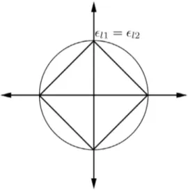
1-ball.

1.3. Bounded energy set

Both

ℓ

1-ball and

ℓ

2-ball are well known sets used in image

reconstruction problems. The

ℓ

1-ball is

C_ℓ1

=

{

∑

n1,n2

|

x

[

n1

,

n2

]| ≤

ϵ

}

(15)

and the

ℓ

2-ball is

C_ℓ2

=

{

∑

n1,n2

|

x

[

n1

,

n2

]|

2

≤

ϵ

2

}

(16)

InFig. 1

ℓ

1and

ℓ

2balls in R2are shown.

Orthogonal projection onto the

ℓ

2ball is implemented by

sim-ply scaling the coefficients of the input vector xj. Let the

∥

xj

∥

2

=

α

2

and

α

2

_{> ϵ}

2_{. The projection x}

j+1of xjonto the

ℓ

2ball is given by

xj+1

=

√

(

ϵ

2

/α

2_)x

Fig. 1.ℓ1andℓ2balls.

The vector xjcan be projected onto the

ℓ

1ball using Duchi et al.’s

method [15]. But it can also be approximately projected onto the

ℓ

1ball in two steps. We first project the current iterate onto the

ℓ

2ball and then to the

ℓ

1ball. For the second step, the projection

vector xj+1obtained by the above equation can be projected onto

the boundary hyperplane of the

ℓ

1ball as follows:

xj+2

=

xj+1

−

∑

n1,n2 xj+1

[

n1

,

n2

] +

ϵ

N (18)

Some of the entries of xj+1may leave the quadrant or RNafter the

above projection operation. We force those coefficients of xj+1to

zero.

1.4. Iterative deconvolution method

The POCS based iterative deconvolution algorithm uses the above projection operations in a successive manner. Let xnbe the

nth iterate. The next iterate xn+1is obtained by

xn+1

=

PFVPℓ1Pℓ2P1,1P1,2

. . .

PL,MPφxn (19)

where PFVrepresents the projection operation onto CFV, Pℓ2

repre-sents the projection operation onto the

ℓ

2ball, Pn1,n2represents the

projection operation onto the hyperplane Cn1,n2and Pφrepresents

the projection operation onto the hyperplane C_φ, and the size of the image is L

×

M. Since all of the sets are closed and convex the

iterates converge to the intersection

Cint

=

Cℓ1

∩

Cℓ2

∩

n1,n2Cn1,n2

∩

Pφ (20)

regardless of the initial input image x1provided that the set Cint

is non-empty. The order of projections in Eq.(19)is immaterial. The convergence speed of iterations can be improved by linearly combining the orthogonal projections [14,16].

We stop the iterations when

∥

xn+1

−

xn

∥ ≤

γ

(21)

where

γ

is a pre-specified number or we stop the iterations after a fixed number of steps.

The proposed method is tested in various datasets and the results are presented in Section3. In the tests, it is observed that the flat background images with less significant Fourier trans-form intrans-formation in higher frequencies show meaningful improve-ments in terms of recovered image quality. Also the recovered

Fig. 2. Flow chart of the proposed algorithm.

image quality is higher in highly blurry images compared to the other well-known deconvolution methods mentioned in this pa-per. These results are parallel to the intended use of the software in microscopic imaging and MPI.

2. Software description

Presented software DeconvApp v2 is a MATLAB function im-plemented on the 2016a version of the program. MATLAB is an engineering tool that has versions for Windows, Linux and MAC environments. The software written makes use of the Image pro-cessing toolbox functions such as conv2 and fft2, therefore this toolbox is required in order to run the software.

In order to make a quick visual comparison with well known Wiener and Lucy–Richardson deconvolution methods, software also displays the deconvolution results of these algorithms.

A demo script which calls blurs an image and calls the presented deconvolution function is also presented. The software that gener-ates the results presented in this paper is also available in Github.

2.1. Software architecture

The application runs in an iterative manner. As input we need a blurry image and the blurring filter and also a limit for the iterations. The iteration number limit is used to break iteration if reached, however we also stop iterations if the consecutive iterates are similar to each other. The similarity measure is the mean-square error of resulting images in each iteration to be lower than a given threshold.

We also require the original image as an input in order to calculate performance factor PSNR.

An outline of the algorithm and related software is given as a flow chart inFig. 2.

Procedure starts by extracting estimate Fourier phase informa-tion from blurry image. The initial estimate for the original image can be a random image. Starting from this initial estimate, Fourier transform phase is recovered from blurry image in Fourier domain and the spatial domain features are restored by

ℓ

1ball projection

iteratively.

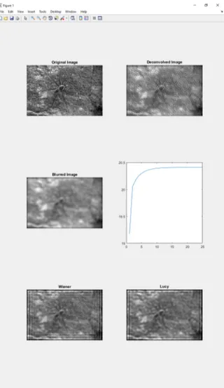
3. Illustrative examples

In the GitHub repository [17], a demo script ‘demo.m’ is pre-sented. This script blurs a test image ‘barbara.png’ and calls the deconvolution function for deblurring the resulting image. Alter-natively projDecon

v

can be called directly for any blurry grayscale image. When we call the demo script a window pops up as shown inFig. 3a.

Fig. 3. (a) projDeconv output as it is processed by MATLAB 2016a. The input is blurred with a disk filter with radius=9 pixels. The added Gaussian noise hasσ =0.01. (b) Command line prints provide information of the current iterate and the PSNR.

Table 1

PSNR comparison of deconvolution algorithms for disk shape filter with various radius r. First four images are from dataset presented in [18] and the last two images are standard test images.

r: Presented software (dB) Wiener deconvolution (dB) Lucy–Richardson method (dB)

6px 9px 12px 6px 9px 12px 6px 9px 12px Im1 22.14 20.88 19.76 19.66 17.99 16.72 20.28 18.91 17.75 Im2 22.25 21.48 20.77 21.91 20.47 19.59 22.55 20.85 19.84 Im3 22.04 21.20 20.23 22.53 20.99 19.74 23.43 21.52 20.06 Im4 25.01 23.29 22.35 21.61 19.89 18.64 22.44 20.49 18.97 Barbara 21.67 21.15 20.65 21.40 20.41 19.73 22.28 21.32 20.18 Lena 24.56 23.80 23.04 23.71 22.29 21.14 25.30 23.56 22.37

In the command window, it is possible to track the current iteration index and the quality of deconvolution in terms of PSNR as shown inFig. 3b.

For blurring the input image, we used a function called ‘blurIm-age’ which is also available in GitHub. We used this function to crop resulting filtered image to prevent border gradient which naturally occurs in convolution operations. With removal of this border effect we better simulate real life blurry images. This may introduce additional complexities in deconvolution problems. The difficulties created by cropped edges are observable in the results of well known deconvolution methods such as Wiener and Lucy– Richardson. However, our software deals with this by artificially generating a gradient using the input filter.

We tested the algorithm with zero noise case as shown inFig. 4. For this we manually modified the code ‘blurImage’ and set std_de

v

variable to 0.

Additionally we tested our software using the dataset presented in [18] and the BSDS500 dataset [19]. These datasets are used in deconvolution and segmentation applications [20,21]. The first dataset that was taken from [18] consists of four images in

.

mat

format. The files include grayscale image matrices as well as a psf and blurred image. The BSDS500 dataset includes 500 color images which we converted to grayscale in order to use as test data. We selected 20 images from this dataset which satisfies a low noise background feature that is essential for meaningful Fourier phase information for recovery. An example of low quality reconstruc-tion is given inFig. 5. We tested these selected images against regularized filter deblurring function of Matlab (′

decon

v

reg′

) [22] also.

As our zero phase assumption requires, we needed to apply our filters to the original images in the datasets. We applied disk and Gaussian filters with changing radius/variance onto the images.

Table 2

PSNR comparison of deconvolution algorithms for Gaussian shape filter. First four images are from dataset presented in [18] and the last two images are test images.

σ: Presented software (dB) Wiener deconvolution (dB) Lucy–Richardson method (dB)

4 7 11 4 7 11 4 7 11 Im1 21.30 20.05 19.84 21.76 17.87 16.49 22.36 19.15 16.94 Im2 21.44 20.62 20.75 22.26 19.88 19.36 22.37 20.48 19.61 Im3 21.21 20.12 20.12 23.15 20.23 19.54 23.06 20.80 20.07 Im4 23.80 22.24 22.02 23.67 19.58 18.23 24.03 20.60 18.09 Barbara 21.34 20.75 20.70 22.16 20.24 19.52 22.41 21.20 20.53 Lena 23.99 23.10 23.08 25.14 21.94 20.80 25.60 23.41 21.96

Fig. 4. ProjDeconv output with zero noise Blurry image. The input is blurred with

a disk filter with radius=9 pixels. Note that even though no additional noise is introduced, border cropping reduces the quality of Fourier Transform phase extraction.

We also applied a Gaussian noise with

σ =

0

.

01. It is important to note that the image pixel value range is 0 to 1.

An example run of the software with an image from dataset [18] is given inFig. 6.

We compared the results of our algorithm with well known Wiener and Lucy–Richardson deconvolution algorithms. We used MATLAB implementations of these algorithms. For Lucy– Richardson we only used the blurry image and the filter, and for the Wiener case, we set the noise parameter to be 0.01. The comparison of results of Barbara, Lena and the dataset of [18] for disk filter with disk sizes 6, 9 and 12 are given in theTable 1.

Fig. 5. Deconvolution results of an image with high total variation values. The

PSNR result of the presented software (20.40 dB) is not as good as the results of Wiener (20.60 dB) or Lucy–Richardson deconvolutions (20.51 dB). In this image the background contains ‘‘random’’ objects. As a result the phase of the image appears to be random. This may be the cause of inferior performance.

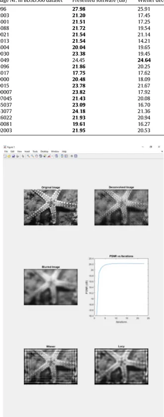
We performed deconvolution over Gaussian blurred images from the same sets. The results of these deconvolution tests are given inTable 2.

A larger test is applied to selected images from BSDS500 database. In this case we compared the results of the proposed method with the results of Wiener, Lucy–Richardson and Reg-ularized filter deblurring. For the last method, Matlab function

′

decon

v

reg′

is used.Table 3presents a small portion of the exten-sive results of the tested images for 13px-radius disk-type blurring filter.

69000 20.48 18.09 18.75 13.57 69015 23.78 21.67 22.25 17.08 100007 23.82 17.92 20.10 13.83 107045 21.43 20.08 20.58 16.85 135037 23_.09 16.70 19.21 11.11 153077 24.18 21.36 21.97 13.29 226022 21.93 20.94 21.08 18.05 260081 19.61 16.27 17.19 13.93 302003 21.95 20.53 20.27 10.79

Fig. 6. ProjDeconv output with Gaussian noise (σ =0.01) Blurry image. The input is image 12003 from BSDS500 dataset blurred with a disk filter with radius=13 px.

Statistical results of all the tests made for different types and scales of blurring psfs are givenTable 4.

FromTables 1and2, we observe that as the amount of blur increases, reduction in output quality in terms of PSNR is the least compared to other two well known deconvolution methods.

Therefore success rates seem to surpass for larger psfs. InTable 4

we see that for flat background images the proposed method outperforms well-known deconvolution methods.

4. Impact

The software provided with this paper and its various versions (Other algorithms that we developed which rely on Fourier trans-form phase) are used in our group for deblurring microscopic im-ages. Recently we applied a similar concept to MPI which produces highly blurry images that are unusable without a proper decon-volution. We observed that even though well known deblurring algorithms such as Wiener and Lucy–Richardson methods may be used in such cases, for high blur conditions, an addition of a phase condition shows great improvement. Therefore we believe the provided software may be preferable in high blur deconvolution problems such as MPI.

The proposed method and accompanying software aims to de-convolve blurry images using projections onto convex sets (POCS). While the

ℓ

1-

ℓ

2ball projections and filtered variation is used in

regularization purposes, the projection onto Fourier phase is per-formed to correct any phase deformations during iterations. The known zero phase psf requirement is a must for the software to proceed correctly.

However the algorithm can be extended to non-zero phase cases by subtracting the phase of the blurring function from the observed image to estimate the phase of the original image.

It is known that rapidly changing images with high total vari-ation has noise-like behavior in their Fourier domain counterpart, resulting in high frequency components in Fourier domain and ran-dom looking phase information after noise addition and cropping. In such cases it may not be always feasible to estimate the phase of the original image in Fourier domain. Therefore it is recommended to use our software in ordinary images including microbiology images and MPI images.

The presented software and its other versions has not been used in commercial settings. The provided software is the only version that is made publicly available. It is made open source and therefore it is possible to modify the code according to the needs of the application.

5. Conclusions

In this paper, we propose a POCS based deconvolution software that takes advantage of Fourier Transform Phase characteristics of

Table 4

Mean PSNR comparison of deconvolution algorithms over 20 images from BSDS500 dataset. Disk filter (dB) Gaussian filter (dB)

r: 6px r: 9px r: 12px σ: 4 σ: 7 σ: 11

Proposed software 24_.10 22_.99 22_.16 23.04 21_.23 20_.03

Wiener deconvolution 21.83 20.49 19.53 22.96 20.67 19.07 Lucy–Richardson method 22.67 21.12 20.17 23.08 21.06 19.63 Regul. filter deconvolution 19.60 17.86 15.65 19.24 17.15 16.38

symmetric blurs. We also use orthogonal projections onto

ℓ

1and

ℓ

2balls and Filtered Variation in order to regularize the restoration

process in each iteration. In addition, we introduce a computa-tionally efficient method to estimate projection onto the

ℓ

1ball

without complicated ordering operations. Ordering the image data is an Order(N) sorting operation but N

=

L2for an image of size L by L.

Our approximate projection consists of two steps. First we make an orthogonal projection onto the

ℓ

2ball which is basically scaling

the data by a constant. Then we make an orthogonal projection onto the boundary hyperplane of the

ℓ

2ball which is an almost

multiplication free operation.

The experimental results show that the provided software out-performs well known Wiener and Lucy–Richardson methods in flat background images with large blur psfs.

References

[1]Trussell H, Civanlar M. The landweber iteration and projection onto convex sets. IEEE Trans Acoust Speech Signal Process 1985;33(6):1632–4.

[2]Youla Dan C, Webb Heywood. Image restoration by the method of convex projections: Part 1: Theory. IEEE Trans Med Imaging 1982;1(2):81–94. [3]Sezan MI, Stark Henry. Image restoration by the method of convex

projec-tions: Part 2-applications and numerical results. IEEE Trans Med Imaging 1982;1(2):95–101.

[4]Chierchia Giovanni, Pustelnik Nelly, Pesquet J-C, Pesquet-Popescu Béatrice. Epigraphical projection and proximal tools for solving constrained convex optimization problems. Signal Image Video Process 2015;9(8):1737–49. [5]Getreuer Pascal. Total variation deconvolution using split Bregman. Image

Process On Line 2012;2:158–74.

[6]Tofighi Mohammad, Yorulmaz Onur, Köse Kivanç, Yıldırım Deniz Cansen, Çetin-Atalay Rengül, Cetin A Enis. Phase and tv based convex sets for blind de-convolution of microscopic images. IEEE J Sel Top Sign Proces 2016;10(1):81– 91.

[7]Yorulmaz Onur, Demirel O Burak, Cukur Tolga, Saritas Emine U, Cetin A Enis. A blind deconvolution technique based on projection onto convex sets for mag-netic particle imaging. IEEE Trans Biomed Eng 2017, Submitted for publication.

[8] Oppenheim Alan V, Lim Jae S. The importance of phase in signals. Proc IEEE 1981;69(5):529–41.

[9] Li Yanjun, Lee Kiryung, Bresler Yoram. Identifiability in blind deconvo-lution with subspace or sparsity constraints. IEEE Trans Inform Theory 2016;62(7):4266–75.

[10] Campisi Patrizio, Egiazarian Karen. Blind image deconvolution: theory and applications. CRC press; 2016.

[11] Rudin Leonid I, Osher Stanley, Fatemi Emad. Nonlinear total variation based noise removal algorithms. Physica D 1992;60(1):259–68.

[12] Perrone Daniele, Favaro Paolo. A clearer picture of total variation blind decon-volution. IEEE Trans Pattern Anal Mach Intell 2016;38(6):1041–55. [13] Tofighi Mohammad, Kose Kivanc, Cetin A Enis. Denoising images corrupted by

impulsive noise using projections onto the epigraph set of the total variation function (pes-tv). Signal Image Video Process 2015;9(1):41–8.

[14] Combettes Patrick L, Pesquet J-C. Image restoration subject to a total variation constraint. IEEE Trans Image Process 2004;13(9):1213–22.

[15] Duchi John, Shalev-Shwartz Shai, Singer Yoram, Chandra Tushar. Efficient projections onto the l 1-ball for learning in high dimensions. In: Proceedings of the 25th international conference on machine learning. ACM; 2008. p. 272–9. [16] Marks II Robert J. Handbook of fourier analysis & its applications. Oxford

University Press; 2009.

[17] Yorulmaz Onur, Cetin A Enis. Github repository for submitted article, GitHub repository, GitHub, 2016 https://github.com/onuryorulmaz/Deconvolution. git.

[18] Levin Anat, Weiss Yair, Durand Fredo, Freeman William T. Understanding and evaluating blind deconvolution algorithms. In: Computer vision and pattern recognition, 2009. CVPR 2009. IEEE conference on. IEEE; 2009. p. 1964–71. [19] Martin D, Fowlkes C, Tal D, Malik J. A database of human segmented natural

images and its application to evaluating segmentation algorithms and mea-suring ecological statistics. In: Proc. 8th Int’l Conf. Computer Vision, vol. 2, p. 416–423.

[20] Levin Anat, Weiss Yair, Durand Fredo, Freeman William T. Understanding blind deconvolution algorithms. IEEE Trans Pattern Anal Mach Intell 2011;33(12): 2354–67.

[21] Sun Libin, Cho Sunghyun, Wang Jue, Hays James. Edge-based blur kernel estimation using patch priors. In: Computational photography (ICCP), 2013 IEEE international conference on. IEEE; 2013. p. 1–8.

[22] The MathWorks Inc. Deblurring images using a regularized filter, 2017https: //www.mathworks.com/help/images/examples/deblurring-images-using-a-regularized-filter.html?prodcode=ML[Online; accessed 25-August-2017 ].