Exact solutions and linearization of modified emden equation

273

ARAŞTIRMA MAKALESİ / RESEARCH ARTICLE

EXACT SOLUTİONS AND LİNEARİZATİON OF MODİFİED EMDEN EQUATİON Özlem ORHAN1

1_{Department of Engineering Basic Sciences, Bandırma Onyedi Eylül University, Balıkesir.} oorhan@bandirma.edu.tr ORCID No: 0000-0003-0058-0431

Bahar MİLANİ2

2_{Department of Computer Engineering, Bandırma Onyedi Eylül University, Balıkesir.} bmilani@bandirma.edu.tr ORCID No: 0000-0002-5295-4215

Muhammed MİLANİ3

3_{Department of Computer Engineering, Bandırma Onyedi Eylül University, Balıkesir.} mmilani@bandirma.edu.tr ORCID No: 0000-0003-2450-0280

GELİŞ TARİHİ/RECEIVED DATE: 27.12.2020 KABUL TARİHİ/ACCEPTED DATE: 28.12.2020

Abstract

In this study, we present that the modified Emden equation has invariant solutions for arbitrary coefficients α and β. Firstly, we demonstrated that modified Emden equation can be linearized. The symmetries of the equation can be derived using a feasible algorithm after this equation is linearized. The exact solutions of the equation are found using a new algorithm and with helping these symmetries. Additionally, finding solutions are classified with respect to the physical meaning of arbitrary coefficients. Finally, all graphics of solutions have been presented with Mathematica and Matlab.

Keywords: Feasible Algorithm, Differential equations, Symmetries, Linearization, Modified Emden equation. MODİFE EDİLMİŞ EMDEN DENKLEMİNİN TAM ÇÖZÜMLERİ VE LİNEERLEŞTİRİLMESİ

Özet

Bu çalışmada, keyfi α ve β katsayılarını içeren modife edilmiş Emden denklemi ele alınmıştır. Öncelikle, modife edilmiş Emden denkleminin lineerleştirilebildiği gösterilmiştir. Bu denklemi lineerleştirdikten sonra, elverişli bir algoritma kullanılarak denklemin simetrileri elde edilmiştir. Bu elde edilen simetriler ve yeni algoritma kullanılarak modife edilmiş Emden denkleminin kesin çözümleri bulunmuştur. Ek olarak, bulunan çözümler içerdikleri keyfi kaysayıların fiziksel anlamlarına göre sınıflandırılmıştır. Son olarak, bulunan çözümler kullanılarak bu çözümlerin zamana göre grafikleri Mathematica ve Matlab programları ile elde edilmiştir.

274

1. Introduction

There are a lot of study in nonlinear dynamics related to the modified Emden type equation, called the modified Painlev´e-Ince equation.

+ x + = 0, (1)

where over dot denotes differentiation with respect to time and α and β are arbitrary parameters. Painlev´e studied the equation (1) and found general solution for two parametric choices β = and β = − Painlev´e (1902) and Ince (1956). Moreover, physicists have demonstrated that the equation (1) has in different meanings and it can be used in the study of equilibrium configurations of a spherical gas cloud acting under the mutual attraction of its molecules and subject to the laws of thermodynamics Moreira (1984) and Chandrasekhar (1957).

The solutions of modifed Emden equation are attracted considerable attention in the literature because these solutions play important role in applied mathematics, physics, and engineering problems. It is understood that obtaining the analytical solution of modified Emden equation is more difficult than the numerical solution. There are some useful methods for solving nonlinear modified Emden equation were appeared in literature Chandrasekhar, Senthilvelan and Lakshmanan (2007).

Symmetry methods is one of these useful methods to investigate differential equations, so many researchers have been studied symmetry methods Noether (1971), Bluman and GW. Kumei (1989), Stephani (1989), Hosseinpour, Milani and Pehlivan (2018), and Orhan (2019).

There are different symmetries and a lot of methods to obtain these symmetries Lie (1883) and Muriel and Romero (2001). Differential equations can be classified as linear and nonlinear differential equations and it is easier to find solutions of linear differential equations. Furthermore, obtaining invariant solutions for nonlinear differential equations is a difficult procedure, while numerical solutions of nonlinear differential equations are easier to obtain.

There are a method to simply these diffucult procedure and this method is called linearization. By this way, nonlinear differential equations can be transformed to linear equation. In this study, linearization methods are examined.

Firstly, we examine how linearization methods are applied. We take the following equation to explain this method

+ (t,x) + (t,x) + (t,x) + (t,x)=0, (2) which is independent variable and is dependent variable of time .

There is first integral of the following form

275 of the equation (2). It was defined a feasible algortihm by Muriel and Romero (2009) to obtain the first

integrals. The coefficient in equation (2) must be zero to find the first integrals of the form (3) using this developing algorithm.

Thus, the equation (2) can be written as

+ (t,x) + (t,x) + (t,x) + (t,x)=0, (4)

First, this algorithm will be examined, To calculate the first integrals of the equation (4), firstly we will consider this algorithm. We will apply defined algorithm to modified Emden equation and thus first integrals, integration factors and solutions of the modified Emden equation will be yield.

2. Steps of Algorithm which is used to Linearize

In this section, we take over feasible algorithm which is given the first integrals of the form

for equations in form (4) and see that the equations can be linearized using these first integral Duarte, Moreira and Santos (1994) and Chandrasekar, Senthilvelan and Lakshmanan (2005). Firstly, the equation should be classified to get the first integrals of the form (3). The following functions and

, (5) and

(6) are calculated to classify equations.

If the function is calculated as zero, then the function must be zero.

On the other hand, If the function then is calculated and seen that it is not equal to zero two new functions and should be defined. The functions and are defined as

, (7)

(8)

In the new calculation, if the function is found as zero, then the function should be obtained as zero. Now, we consider the algortihm which is given first integrals under these classification.

276

Under this case, firstly the derivatives of the function is written as

, and (9) In the next step of algorithm, the function is calculated using first step.

In the following step, the function is given as

, (10) Using the equation (10), the function can be derived.

In the fourth step, the following differential equation

, (11)

is given. And if we substitute the obtaining function in the equation (11) , then we can obtain the function solving the equation (11).

In the fifth step, the derivatives of the function are accepted in the following form

and (12) and if the equation (12) is solved, then the function Q is derived.

In the last step, the functions and are yield as the following form

and (13) Finally, it can be seen that the first integral of the form are evaluated.

Additionaly, the exact solution of the equation (4) can be yield using first integral which is given in the form of (3).

Case II: If the function , the functions and should be zero. If the equation (4) is classified in this case, we should apply the following steps. Firstly, the function is computed as

277 Then, the function is found using the following equations

and (15) The function and is defined as

and (16) In the next step, we can find first integral using finding functions.

Finally, the exact solutions can be obtained by first integrals. 3. The exact solutions for modified Emden Equation

In this section, firstly the modified Emden equation will be classified. Then, using the algorithm which is defined in the previous section we will compute first integrals and analytic solutions.

The modified Emden equation is defined as

(17)

where x is the position coordinate which is a function of the time t, and is a scalar parameter indicating the nonlinearity and the strength of the damping Chandrasekhar, Senthilvelan and Lakshmanan (2007). To obtain first integral of the equation (17), we apply the algorithm which is mentioned previous section. Before applying this feasible algorithm, we should classify this equation.

We should compute the functions , and to classify equation (17).

Before this classification, we take special form of the equation (17) for the coefficient choices. Case I: For the coefficient .

In this situation, the equation (17) is converted to

(18) To classify the equation (18), the function is found

(19)

It is seen that the function . We know that from the theorem, if the function , then the functions and must be equal to zero to be linearized the equation (14).

278

Therefore, we calculate the following functions

, and (20) We know that the function and should be zero, so the coefficient should be zero.

Thus, we can say that the modified Emdenl equation can be linearized by using step by step algorithm which is mentioned in the previous section.

The equation is classified, the algorithm that gives the first integral can now be applied. If we replace the coefficients in equation (9) and (10) and solving these equations, the functions

and (21) are obtained.

Thus, the functions of and

and (22) Furthermore, the first integral of the equation (17) is

(23) where is arbitrary function.

Using the first integral (23), the analytic solution of the equation (18)

(24) where and are arbitrary functions.

Case II: For the selection .

For this selection, the equation (17) is transformed to

(25) To classify the equation (25), the function is found as

and (26)

279 We compute and see that the functions and are equal to zero. Thus, equation (25) can be linearized.

Now, we can apply steps of algorithm.

In the first step, the function is computed using coeeficients and ti seen that it is equail to zero. In the second step, we obtain the function

(27) Thus, the functions and

and (28) are found. Finally, the first integral of the equation (25) is yield as

(29) Using first integral (28), the analytic solution of the equation (24)

(30) where and are arbitrary numbers.

Now, we examine phase portrait for modified Emden equation. To simply solution (30), we chose

. We can select different arbitrary numbers. Then we calculate the solutions for choices , , , respectively and so we obtain the following graphic which in time parameter t changes according to x coordinate.

280 0.6 0.4 0.2 0.2 0.4 0.6 t 0.4 0.6 0.8 1.0 x

Fig. 1. Solution plot of analytic solution (30) for the choices , , , .

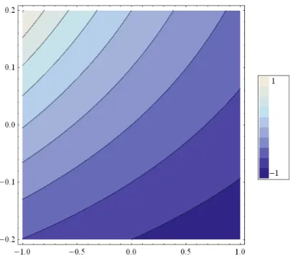
281 In the Figure 2, we arbitrary coefficient changes from -1 to 1.We can see that change of solution (30)

according to time in this interval of . Conclusions

In this study, firstly, the modified Emden equation is classified by computing functions. It is shown that the functions and are not equal to zero. Therefore, the functions and are computed and it can be seen that the function is equal to zero. It is known that if the function is equal to zero, then the function must be zero. Thus, we equalize the function to zero. We demonstrated that the modified Emden equation has the second class and so we should use algorithm which is defined in case II. Using this algorithm, it was presented that how to classify ordinary differential equations and to obtain exact solutions. It is examined that this classification gives us an algorithm to find the first integrals. By this algorithm, the first integral of the modified Emden equation was obtained. Finally, the phase portraits of the equation are given using some computer programming.

References

Bluman, S. and G.W. Kumei. 1989. Symmetries and Differential Equations, Springer-Verlag, New York. Chandrasekhar, S. 1957. An Introduction to the Study of Stellar Structure (New York: Dover); Dixon J M and Tuszynski J A 1990 Phys. Rev. A 41 4166.

Chandrasekhar, V.K., M. Senthilvelan, and M. Lakshmanan. 2005. On the complete integrability and linearization of certain second-order nonlinear ordinary differential equations, Proceedings of the Royal Society A, 461, 2451-2476.

Chandrasekhar V.K., M. Senthilvelan, and M. Lakshmanan. 2007. On the General Solutions for the Modified Emden Type Equation, Journal of Physics A Mathematical and Theoretical, 40(18), 4717. Duarte L.G.S., I.C. Moreira, and F.C. Santos. 1994. “Linearization under non-point transformation”, J. Phys. A:Math. Gen, vol. 27, pp. 739-743.

Hosseinpour S., M. Alavi Milani, and H. Pehlivan. 2018. Step by step solution methodology for mathematical expressions, Symmetry, 10(7), 285.

Ince E.L. 1956. Ordinary Differential Equations, Dover, New York.

Lie S. 1883. Klassifikation and integration von gewhnlichen differentialgleichungen zwischen x; y, eine gruppe von transformationen gestatten, III, Arch. Mat. Naturvidenskab. Cambridge, 8, 371-458.

Moreira I.C. 1984. Hadronic Journal, 7, 475.

Muriel M. and J.L. Romero. 2001. New methods of reduction for ordinary differential equations, IMA Journal of Applied Mathematics, 66, 111-125.

282

Muriel, M. and J.L. Romero. 2009. Second-Order Ordinary Differential Equations and First Integrals of The Form A(t; x) +B(t; x), Journal of Nonlinear Mathematical Physics, 16, 209-222.

Noether, E. 1971. Invariante Variationsprobleme, Nachr. König. Gesell. Wissen. Göttingen, Math.-Phys. Kl. Heft, 2, 235-257, 1918. English translation in Transport Theory and Statistical Physics, 13, pp. 186-207. Orhan O. 2019. The Modeling of Psychotropic Bacteria Affecting Milk Products. Electronic Letters on Science and Engineering, 15(3), 95-100.

Painleve P. 1902. Sur les équations différentielles du second ordre et d’ordre supérieur dont l’intégrale générale est uniforme, Acta Mathematica. 25, 1-85.

Stephani H. 1989. Differential Equations and Their Solutions Using Symmetries, Cambridge University Press, Cambridge.