i
ANALYSIS OF THE IN-VITRO
NANOPARTICLE-CELL INTERACTIONS VIA SMOOTHING SPLINES
MIXED EFFECTS MODEL
A THESIS
SUBMITTED TO THE DEPARTMENT OF INDUSTRIAL ENGINEERING AND THE GRADUATE SCHOOL OF ENGINEERING AND SCIENCE
OF BILKENT UNIVERSITY
IN PARTIAL FULFILLMENT OF THE REQUIREMENTS FOR THE DEGREE OF
MASTER OF SCIENCE
By
Elifnur Doğruöz
July, 2013
ii
I certify that I have read this thesis and that in my opinion it is fully adequate, in scope and in quality, as a thesis for the degree of Master of Science.
___________________________________ Assoc. Prof. Dr. Savaş Dayanık
I certify that I have read this thesis and that in my opinion it is fully adequate, in scope and in quality, as a thesis for the degree of Master of Science.
___________________________________ Prof. Dr. İhsan Sabuncuoğlu
I certify that I have read this thesis and that in my opinion it is fully adequate, in scope and in quality, as a thesis for the degree of Master of Science.
___________________________________ Assoc. Prof. Dr. Oğuzhan Alagöz
I certify that I have read this thesis and that in my opinion it is fully adequate, in scope and in quality, as a thesis for the degree of Master of Science.
___________________________________ Asst. Prof. Dr. Emre Nadar
Approved for the Graduate School of Engineering and Science: ___________________________________
Prof. Dr. Levent Onural Director of the Graduate School
iii
ABSTRACT
ANALYSIS OF THE IN-VITRO NANOPARTICLE-CELL
INTERACTIONS VIA SMOOTHING SPLINES MIXED
EFFECTS MODEL
Elifnur DoğruözM.S. in Industrial Engineering Supervisor: Assoc. Prof. Dr. Savaş Dayanık Co-Supervisor: Prof. Dr. İhsan Sabuncuoğlu
July, 2013
A mixed effects statistical model is developed to understand the nanoparticle(NP)-cell interactions and predict the nanoparticle(NP)-cellular uptake rate of NPs. NP-nanoparticle(NP)-cell interactions are crucial for targeted drug delivery systems, cell-level diagnosis, and cancer treatment. The NP cellular uptake depends on the size, charge, chemical structure, concentration of NPs, and incubation time. The vast number of combinations of those variable values disallows a comprehensive experimental study of NP-cell interactions. A mathematical model can, however, generalize the findings from some limited number of carefully designed experiments and can be used for the simulation of NP uptake rates for the alternative treatment design, planning, and comparisons. We propose a mathematical model based on the data obtained from in-vitro NP-healthy cell experiments conducted by the Nanomedicine and Advanced Technologies Research Center in Turkey. The proposed model predicts the cellular uptake rate of Silica, polymethyl methacrylate, and polylactic acid NPs given the incubation time, size, charge and concentration of NPs. This study implements the mixed model methodology in nanomedicine area for the first time and is the first mathematical model that predicts NP cellular uptake rate based on sound statistical principles. Our model provides a cost effective tool for researchers developing targeted drug delivery systems.
Keywords: Nanomedicine, targeted drug delivery, nanoparticle uptake rate, linear
iv
ÖZET
DÜZLEME ÇİZGİLERİ KARMA ETKİLER MODELİ
İLE İN-VİTRO NANOPARTİKÜL-HÜCRE
ETKİLEŞİMİNİN ANALİZİ
Elifnur DoğruözEndüstri Mühendisliği, Yüksek Lisans Tez Yöneticisi: Doç. Dr. Savaş Dayanık
Tez Yardımcı Yöneticisi: Prof. Dr. İhsan Sabuncuoğlu
Temmuz, 2013
Bu tezde, nanopartikül (NP)-hücre etkileşimini anlamak ve nanopartiküllerin hücreye tutunma oranını tahmin etmek için bir karma etkiler modeli geliştirilmiştir. NP-hücre etkileşiminin incelenmesi, güdümlü ilaç dağıtım sistemleri ve kanser gibi hastalıkların hücre düzeyinde teşhis ve tedavisi açısından çok önemlidir. Nanopartiküllerin hücreye tutunma oranı, nanopartiküllerin kimyasal yapısı (tipi), boyutu, yüzey yükü ve yoğunluğu ile enkübasyon zamanına bağlıdır. Bu değişken değerlerin çok sayıda kombinasyonu olduğu düşünüldüğünde NP-hücre etkileşiminin kapsamlı bir deneysel çalışmayla incelenmesi pratik bir yaklaşım değildir. Fakat matematiksel bir model, sınırlı sayıda ve dikkatli tasarlanmış deneylerin sonuçlarını genelleyebilmekte ve alternatif işlem tasarımı, planlanması ve karşılaştırması çalışmalarında hücreye tutunma oranı verisinin simulasyonunda kullanılabilmektedir. Bu tezde, Türkiye’deki Nanotıp ve İleri Teknolojiler Merkezi’nin gerçekleştirdirdiği in-vitro NP-sağlıklı hücre deneylerinden elde edilen verilere dayanılarak NP hücresel tutunma oranı için yeni bir matematiksel model önermekteyiz. Önerilen model, her biri küresel şekilli polimetil metakrilat (PMMA), silika ve polilaktik asit (PLA) nanopartiküllerin hücreye tutunma oranını tahmin etmektedir. Bildiğimiz kadarıyla bu çalışma, karma model metodolojisini nanotıp alanında uygulayan ilk çalışma ve NP hücresel tutunma oranını güvenilir istatistiksel prensiplere dayanarak tahmin eden ilk matematiksel modeldir. Bizim modelimiz, güdümlü ilaç dağıtım sistemleri üzerine çalışan araştırmacılar için maliyet etkin bir araç sağlayacaktır.
Anahtar Sözcükler: Nanotıp, güdümlü ilaç dağıtımı, nanopartikül hücresel tutunma
v
Acknowledgement
Foremost, I am deeply grateful to my advisors Prof. Dr. İhsan Sabuncuoğlu and Assoc. Prof. Dr. Savaş Dayanık for their directions and constructive criticism throughout this study, which provided me with the precious enlightenment of the thesis problem during all the work. Without their guidance and persistent help, this thesis would not have been possible. I also place on record my sincere gratitude to Assoc. Prof. Dr. Gürer Budak for his help to NPs production, characterization, cell culture application, and his valuable knowledge and insights to interpretation of experimental results.
I owe a special debt to my dear friends Sibel Sözüer and Pelin Balcı. During my master study, they made me have great time that I will never forget. I also thank Selin Özokcu for her friendship and trust for years. Without their support, everything would have been more difficult.
I am also grateful to TÜBİTAK for providing the financial support.
Finally, I would like to thank my sister, mom, and dad for their infinite support throughout my life.
vi
Contents
1 Introduction 1
2 Literature Review 5
3 Background on Cell Physiology 10 4 Background on Smoothing Splines and Mixed Effects Models 17
4.1. A Brief Description of Smoothing and Mixed Models 19
4.2 Experimental Procedure of Proposed Study 29
5 Proposed Model 32 5.1. Proposed Model for Silica Nanoparticles 34
5.2. Proposed Model for PMMA Nanoparticles 42
5.3. Proposed Model for PLA Nanoparticles 49
5.4. Derivation of Prediction Intervals 53
6 Comparison and Discussion 55 7 Conclusion 66
vii
List of Figures
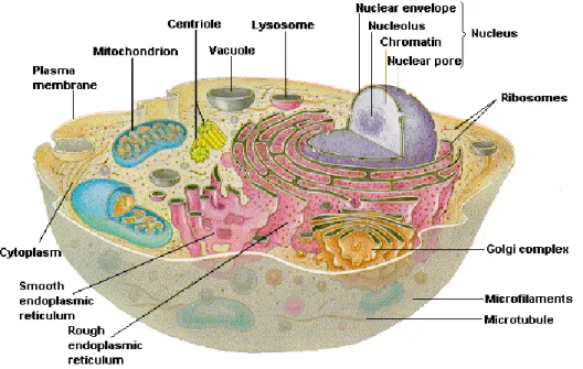
Figure 1: Structure of a typical eukaryotic cell ……….11
Figure 2: Cell membrane ………...13
Figure 3: Endocytosis and exocytosis of a food particle ………...15
Figure 4: Linear regression model ……….20
Figure 5: Quadratic model ……….21
Figure 6: Broken stick model ……….………22
Figure 7: Whip model ………23
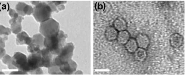
Figure 8: TEM micrographs of (a) iron oxide nanoparticles and (b) CPMV nanoparticle………...31
Figure 9: Silica 50 nm predictions ……….………40
Figure 10: Silica 100 nm predictions ……….…………..………..41
Figure 11: PMMA 50 nm predictions ………47
Figure 12: PMMA 100 nm predictions……….. 48
viii
Figure 14: Silica 50 nm predictions of our model and Cenk et al.’s model ………..…...59
Figure 15: Silica 100 nm predictions of our model and Cenk et al.’s model ……….60
Figure 16: PMMA 50 nm predictions of our model and Cenk et al.’s model ……….61
Figure 17: PMMA 100 nm predictions of our model and Cenk et al.’s model ……….62
Figure 18: PLA predictions of our model and Cenk et al.’s model ……….63
ix
List of Tables
Table 1: Nanoparticle characteristics………...………...33 Table 2: Experimental groups of Silica and PMMA nanoparticles ………...34
1
Chapter 1
Introduction
Cancer is a disease that causes cells to change, grow, and spread uncontrollably. It may affect almost any part of the body. Most types of cancer form a mass called tumor, and the cancer is named according to the place of the tumor. Cancer is the leading cause of death in the world. Breast cancer is the most frequent cancer type among women and the most frequent cause of cancer death in women. It is the fifth cause of deaths from cancer overall in 2008 according to the report of International Agency for Research of Cancer. In 2008, 7.6 million, which is around 13% of all deaths, people died from cancer. It is estimated that 1,660,290 new cancer cases and 580,350 cancer deaths will occur in 2013 only in the United States (Siegel et al., 2013). Moreover, it is expected that deaths from cancer will rise to over 13.1 million in 2030 (Boyle and Levin, 2008).
Cancer was considered incurable before. Some patients can be treated now due to the improved diagnostic techniques and treatments. Current cancer treatment methods involve surgical intervention, radiation, and chemotherapy. However, those methods often harm also the healthy cells and cause toxicity. Therefore, there has been an interest to combine the power of nanotechnology and cancer biology to find
2
new solutions to the cancer In order to provide a less harmful and more effective solution, some research have focused on developing targeted nanoparticles that can directly deliver drugs to cancer cells. In addition to delivering therapeutics, nanoparticles can be used for imaging to detect the disease early at-cell level, and help us understand the tumor biology (Grodzinski, 2011). Moreover, a new method called theragnostics, which combines therapeutics with diagnostics, is developed to have patient-specific treatments. Use of nanoparticles has led the advances in theragnostics (Fang and Zhang, 2010). All of these fields require the use of nanoparticles at cell-level. Therefore, a careful investigation of NP-cell interaction and the cellular uptake process is very necessary to advance the relevant studies.
Our study aims to investigate the cellular uptake rate of nanoparticles (NP) via statistical smoothing and mixed models methodology. Data obtained from in-vitro NP-cell interaction experiments are used to fit penalized spline smoothing model, formulated as a mixed model. The proposed model predicts the cellular uptake rate of NPs having different characteristics. Those characteristics are size, shape, chemical structure (type), surface charge of NPs, and the concentration of NP solutions used. Although some configurations of those characteristics cannot be produced due to technical limitations, the number of the remaining configurations is still vast. Therefore, it is very costly and time consuming to conduct experiments with all those possible configurations. However, prediction of the cellular uptake is still possible by using strong mathematical models. The ultimate aim is to obtain NP
3
specifications with the desired uptake efficiency. Our study was carried out to achieve that aim.
We model the uptake rates of each type of nanoparticle (Silica, polymethyl methacrylate (PMMA), and polylactic acid (PLA)) into the cell in 48-hour time interval by means of a penalized spline smoothing mixed effects model. For each type of NP (Silica, PMMA, and PLA), we develop a model that takes NP size, charge, concentration, and incubation time as inputs to predict the cellular uptake rate. Our model is based on data obtained from in-vitro experiments conducted by the Nanomedicine & Advanced Technologies Research Center in Turkey. Three types of sphere-shaped nanoparticles are used in the experiments. Silica and PMMA NPs were produced in 50 and 100 nm diameter and PLA NPs were produced in 250 nm diameter. For each type and size, NPs were produced with positive and negative surface charges. NP solutions with 0.001 mg/l and 0.01 mg/l concentrations were prepared and added to healthy cell cultures. The number of NPs removed from the environment was counted at 3, 6, 12, 24, and 48 hours of incubation. The difference between the number of NPs added to and removed from the environment is calculated as the number of NPs penetrated into the cell or attached to the cell surface. An experiment was repeated six times for each different configuration of NP characteristics. For Silica NPs, the experiments are replicated for all combinations of size, charge, and solution concentration. Observations are taken at different time points in the second replication. Also, PMMA experiments conducted with positively charged NP solutions of 0.001 mg/l and 0.01 mg/l are replicated, and observations
4
are taken at the same time points in both replications. Having correlated data coming from more than one replication is the main reason why we prefer mixed model to represent this uptake process.
To the best of our knowledge, this study is the first application of penalized smoothing mixed effect model to nanomedicine and is the first random-effect statistical model of NP cellular uptake rate. A closely related study was Cenk et al.’s (2014) Artificial Neural Network model. Unlike that model, our model brings an easy-to-understand explanation to the interactions of various effects on uptake rate, and is capable of linking the data obtained at different times by means of the random effects. The easy-to-interpret components of our model will make the researchers work more comfortably with the model.
The remainder of the thesis is organized as follows: In Chapter 2, the literature on NP-cell interaction is given. In Chapter 3, background about the cell structure and particle transportation is explained for the readers who do not have knowledge about the cell physiology. Our methodology and design of experiments are discussed in Chapter 4. Chapter 5 presents our model. The results are analyzed and compared with the previous studies in Chapter 6. Chapter 7 concludes.
5
Chapter 2
Literature Review
Numerous experimental studies have been conducted to explore nanoparticle-cell interaction in the past few years. In those studies, effects of NP size, surface charge, concentration, chemical structure, and incubation time on the NP-cell interaction are investigated. Most of those studies contain no mathematical model of NP-cell interaction, but provide general comments about the influence of some of the properties of NPs.
Davda and Labhasetwar (2001) investigate the uptake of nanoparticles by endothelial cells in cell culture. They demonstrate that the cellular uptake of nanoparticles depends on the concentration of the nanoparticles in the medium, and the uptake increases with the increase in the concentration. Another result of their study is that the uptake also depends on the incubation time. They image the cells at 0, 30, 60 and 120 minutes from the beginning of the incubation and observe that the uptake increases with the incubation time Their research also shows the biocompatibility of the NPs with cells and usability of NPs to target drugs into the endothelium. Hence, it is a significant study for the targeted drug delivery literature. Besides, this study is also important for us since it shows that
6
the concentration is influential on the uptake of NPs. However, its scope is narrower than our study since they observe only the effect of the concentration of NPs.
Chithrani et al. (2006) study the cellular uptake of colloidal gold nanoparticles by mammalian cells and observe the effects of NP size, shape, and incubation time on the cellular uptake kinetics. They use spherical and rod-shaped NPs with diameters of 14, 30, 50, 74 and 100 nm and length by width of 40x14 nm and 74x14 nm, respectively. They show that maximum uptake occurs with NPs of 50 nm. They also observe that the uptake increases in first 2 hours abruptly and then reaches to a steady level at 4-7 hours, depending on the size. Another result obtained is that the uptake is also dependent on the shape of NP, and more spherical NPs are absorbed to cell more than the rod-shaped counterparts. Their results demonstrate that the drug delivery via NPs can be controlled by adjusting the size and shape of NP. However, no mathematical function is developed to explain the interaction. Moreover, the influence of surface charge and concentration of NPs are not examined in this study, distinctively from our research.
Peetla and Labhasetwar (2007) investigate the effects of surface chemistry of NPs on the interaction between nanoparticles and endothelial model cell membrane. They use polystyrene NPs of different surface chemistry and sizes and observe the changes in the membrane’s surface pressure as a measure of interaction. They utilize aminated, carboxylated and plain (without any surface
7
group) polysterene NPs of 60 nm size. They observe that aminated NPs increase the surface pressure while plain NPs decrease and carboxylated NPs do not change it. They also study the effect of the size of NPs, and show that the smaller NPs increase the surface pressure. They could not compare the effect of 20 nm aminated NPs with the same sized plain and carboxylated NPs since 20 nm aminated NP is not available. They conclude that small aminated NPs and plain NPs have greater interactions with the endothelial model cell membrane than carboxylated and large, plain NPs do. No mathematical model of cellular uptake is developed in this study. However, this research is significant for us since it emphasizes the importance of chemical structure and size of NPs.
Lin et al. (2010) examines the interactions of gold nanoparticles with model lipid membranes by means of coarse-grained molecular dynamics simulation. They state that cationic (positively charged) gold NPs have a higher membrane adhesion than anionic (negatively charged) NPs on a typical mammalian cell membrane since the membrane has an overall electronegative feature. They also reveal that the penetration increases as the charge density, which is the amount of electric charge present on per unit surface area, of NPs increases. Their results demonstrate that the cellular uptake rate can be increased by increasing NP surface charges densities. Although this study does not consider the influence of NP properties except surface charge, it is important for us because the surface charge, which is an input of our study, is proven to be effective on the cellular uptake.
8
In the previously mentioned studies, NP-cell interaction is only explored through observations collected from physical experiments. Although they shed light on the role of various NP properties in the NP-cell interaction, none of them describe a mathematical model that relates the properties of NPs to the NP-cell interaction. Hence, they are incapable of predicting the cellular uptake rate, which is the aim of our research. Besides, none of the previous studies investigate the interactions between different NP properties (chemical structure, size, charge and concentration of NPs) as they concurrently act, as we do in our study.
In one of very few studies proposing some mathematical models, Boso et al. (2011) try to identify the optimal configuration that maximizes the NP accumulation at the diseased site via developing a mathematical model. They conduct a parallel plate flow chamber in vitro experiment with spherical polystyrene NPs. Based on the data obtained from the flow chamber experiments; they develop an artificial neural networks model (ANN) to predict the number of NPs adhering to the vasculature as a function of shear rate and NP diameter. They show that an optimal particle diameter exists for which the number of NPs adhering to the vessel walls is maximized. That optimal diameter depends on the wall shear rate, which is controlled through the syringe pump flow rate. This study investigates the effects of only the NP size and the wall shear rate on the NP accumulation. The other properties of NPs such as type, charge and concentration are not considered. However, they do not use real cells. Although the scope of the study is very limited, it shows that mathematical models can help minimize the
9
number of experiments otherwise needed to adequately understand NP-cell interaction, which is the motivation of this research.
Another mathematical model is proposed by Cenk et al (2014). They investigate the NP-cell relations regarding the effects of NP size, surface charge, concentration, and chemical structure. They develop an artificial neural networks model to predict the cellular uptake by utilizing the same data set used in our study. Smoothing with linear mixed models is often preferred over artificial neural networks because the latter are considered as black boxes and their outputs are harder to interpret. Furthermore, when experiments are replicated, as in the cases for Silica and PMMA nanoparticles in our experiments, mixed model approach allows them to be naturally tied to a single model by means of suitable random effects.
Although mixed model approach has not been used in nanomedicine area until now, it has been widely used to analyze clustered medical data. Mixed models can handle clustering effects by modeling them as random variables. Mixed models can also tolerate to missing data (Brown and Prescott, 2006). Moreover, mixed models are appropriate for modeling complex input-output relations such as NP-cell interaction. To the best of our knowledge, our study is the first to propose a linear mixed model for cellular uptake rate. We expect that our new model will advance the research in targeted drug delivery. It contributes to applied statistics as a novel application of mixed models.
10
Chapter 3
Background on Cell Physiology
In the experiments conducted for this research, the target is to observe the NP-cell interactions. Hence, NP solutions are added to NP-cell culture plates, and number of NPs adhered on or penetrated into the cell is calculated. To understand the experiments and interpret the results physiologically, it is crucial to understand the dynamics of the cells and particle transportation process. In this chapter, basic information about the cell structure and particle transportation will be given for the typical audience considered as engineers and statisticians. Readers who have knowledge about those topics may skip this chapter.
Cells are the basic functional units of living organisms. They are small but complex structures. Cells join together to create tissues, which organs are made up of. There are about 100 trillion cells in the human body (Guyton and Hall, 2006). There are many types of cells such as nerve cells, blood cells, muscle cells, bone cells. Cells differ from each other both morphologically and metabolically. While some bacteria can be seen hardly in the light microscope, some neurons might have a size of 1 meter.
11
Despite of the differences in sizes, shapes, and activities, all cells have two main functional regions: the nucleus and the cytoplasm (Wolfe, 1999). The nucleus contains and transmits the genetic material needed for cell growth and reproduction. It is separated from the cytoplasm by a nuclear membrane. The cytoplasm uses the information stored in the nucleus to grow and reproduce. It also provides the energy to maintain these activities. The cytoplasm is separated from the fluids surrounding the cell (extracellular fluids) by the cell membrane. The cell contains highly organized physical subunits, which have specific functions, called organelles. Ribosome, mitochondria, endoplasmic reticulum, Golgi complex, lysosome are some of the organelles in the cells. Figure 1 shows a typical eukaryotic animal cell (Chiras, 2011). Some of these organelles have membranes; hence, they divide the cell into compartments.
12
Cells are organized by the systems of membranes. The cell membrane, which completely envelops the cell, is very important because the cell has to separate itself from the outside due to two reasons. First reason is that the cell must protect DNA, RNA, and other molecules from dispersion. Second reason is that the foreign materials that may be harmful must be kept away. While accomplishing these, the cell also should communicate with the outside, and accommodate itself to the changes in the environment. The cell membrane functions as a contact region with the outside world. Necessary substances and raw materials enter cells; waste and toxic materials are removed from the cell through the cell membrane.
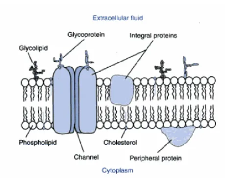
The cell membrane is a thin and elastic structure having about 7.5 to 10 nanometers thickness, and is mostly composed of proteins and lipids (Guyton and Hall, 2006). It also contains carbohydrates combined with proteins and lipids in the form of glycoproteins and glycolipids (Rhoades and Bell, 2009; see Figure 2). Lipid bilayer is the framework of the membrane. Proteins are embedded as individual units in or on the bilayer. This lipid bilayer is impermeable to water-soluble substances such as glucose, urea, and ions whereas it is permeable to fat-soluble substances such as oxygen and carbon dioxide. There are integral and peripheral proteins in the membrane. Integral proteins are embedded to the lipid bilayer partly or completely, and they are suspended in the lipid bilayer. Peripheral proteins are attached to the membrane surfaces. Integral proteins function in the particle transportation by forming pores through which water-soluble substances can diffuse between the inside and outside fluids of the cell or by carrying substances in the opposite
13
direction of the diffusion. Peripheral proteins are generally attached to integral proteins. They function as enzymes or control intercellular activities in different ways.
Figure 2: Cell membrane (Rhoades and Bell, 2009)
There are two main mechanisms for particle transportation across the membrane: passive transport and active transport. Basically, if a particle passes the membrane without using cellular energy, it is called passive transport. Otherwise, the cellular energy is used, and it is called active transportation. Diffusion and osmosis are examples of passive transport. Diffusion is the movement of ions or molecules from a region with high concentration to a region with low concentration without expending the cellular energy. The rate of the movement depends on the difference between the concentrations, called concentration gradient; the movement continues
14
until the molecules are evenly distributed in both regions. Diffusion has two subtypes: simple diffusion and facilitated diffusion. Simple diffusion is kinetic movement of molecules or ions through an opening in the lipid bilayer or watery channels of some transport proteins (Guyton and Hall, 2006). On the other hand, in the facilitated diffusion, the particles pass through the membrane with the help of carrier proteins. The factors affecting the diffusion rate are:
Membrane permeability: This means the rate of diffusion of molecules across
the cell membrane. Various factors affect the membrane permeability. These are thickness of the membrane, number of protein channels appropriate for the molecule per unit area, lipid solubility, and weight of the molecule and temperature.
Concentration difference: The rate of diffusion is proportional to the
concentration difference.
Electrical potential: Electrical potential causes particles to move even if there
is no concentration difference. This situation triggers the occurrence of concentration difference. Diffusion continues until these two forces, electrical potential and concentration gradient, balance each other.
Osmosis is simply the diffusion of the water through the cell membrane. The movement of water is again caused by concentration difference.
In active transport, molecules or ions are moved inside or outside of the cell against the concentration gradient in contrast to the passive transport. Therefore, the cellular energy in the form of ATP (adenosine triphosphate) is used. Sodium and
15
potassium ions, calcium ions, iron ions, different sugars, and amino acids are some of the substances transported actively (Guyton and Hall, 2006).
Active and passive transport permit the passage of the small molecules between inside and outside of the cell. However, cells also need to take and remove larger molecules like proteins and nucleic acids (Wolfe, 1999). Taking large materials from outside to the inside of the cell is called endocytosis. Firstly, the molecule that will be taken inside is connected to the membrane surface via receptors. Then, the membrane invagination occurs and a vesicle is formed around the molecule. Generally, the enzymes break down the vesicle in cytoplasm. For example, white blood cells engulf bacteria via endocytosis. Also, nanoparticles may be taken into the cell via endocytosis. The reverse mechanism of endocytosis is called exocytosis. It provides the release of big molecules to the outside of the cell. After the molecule is surrounded by a membrane and vesicle is formed, it is carried to the cell membrane. It unites to the membrane and then the vesicle is released to the outside. Figure 3 shows endocytosis of a food particle and then exocytosis after digestion (Purves et al., 1994). Both endocytosis and exocytosis require the use of the cellular energy.
16
17
Chapter 4
Background on Smoothing Splines and Mixed
Effects Models
Cancer is a widespread disease that results in death if its spread is not prevented. Most cancers are treated by surgery, chemotherapy and radiotherapy today. However, these treatment methods are not very efficient because they are not capable of removing all tumor cells. Also, generally healthy cells are damaged in the treatment process. Therefore, there has been a developing interest to targeted drug delivery systems to kill tumor cells without harming healthy ones in recent years. In this context, nanoparticles with their abilities to store drugs in their cores and targeting properties become very suitable tools for that aim.
The effective use of nanoparticles in targeted drug delivery depends on the knowledge of the interaction between the cells and NPs. The cellular uptake of NPs depends on the NP size, shape, surface charge, chemical structure and concentration. However, it is impractical to conduct all experiments with many different values of those variables. Moreover, analysis of the experimental data is complex because of the statistically fluctuating environment of living organisms. Hence, the most efficient and reliable synthesis of the interaction data is a well-thought
18
statistical/mathematical model of the complex relation between the cell uptake rate and NP characteristics. In this research, for each type of nanoparticles (Silica, PMMA, and PLA), we model the percentage of NPs entered in or attached to the cells in 48-hours time interval as a function of size, charge, and density of NPs. We use the smoothing mixed model approach. Mixed models are designed to handle both fixed and random effects. Fixed effects are population-averaged parameters and influence average cellular NP uptake rate while random effects address variabilities in cellular NP uptake rate due to different cases under the same treatments. Mixed models can also naturally handle semiparametric smoothing that is able to capture nonlinear relationships between predictors and NP cellular uptake rate. We prefer semiparametric smoothing because it can capture important local variations in uptake rates. Besides, the replicated experiments with Silica and PMMA NPs can be treated most naturally with random effects in mixed-effect model setup. Those replications are similar to subjects selected at random from the same population. If we fit a model for each replication, we need to estimate too many parameters and then estimates will be less accurate. We also need a meaningful model of future realizations as well as the past observations. Mixed models can fulfill those requirements.
In the Section 4.1, a brief description of smoothing and mixed models is given. Readers with detailed knowledge of mixed models and smoothing may skip this section. In Section 4.2, experimental procedure of the proposed study and NP-cell interaction data used in the model is explained.
19
4.1 A Brief Description of Smoothing and Mixed Models
4.1.1 Smoothing
Scatter plots are simply the collections of some points on a plane, without any connection to a probabilistic model (Ruppert et al., 2003). Scatter plot smoothing is a widely used data analysis technique when the aim is to find the underlying trend in the scatter plot. When looking at the scatter plot, we can think the vertical positions of the points as realizations of a random variable y (response variable) that is conditional on the horizontal position of the point x (explanatory variable). For example, a scatter plot may represent the relation between the years of education (x) and the annual income (y). Then we can write
. (4.1)
Equation (4.1) can also be written as
where . (4.2) Here, is a smooth function, and it should be estimated from and . There are many ways to fit a smooth curve to a set of noisy observations and the penalized
splines method is one way of doing this.
4.1.1.1 Penalized Splines (P-Splines)
Consider the linear regression model displayed in Figure 4, where the horizontal axis represents predictor variable x and the vertical axis represents response variable
20
(4.3)
which can be expressed compactly as ,
where , , and the X-matrix for fitting regression is
. For
the model in (4.3), the functions 1 and x are the corresponding basis.
Figure 4: Linear regression model
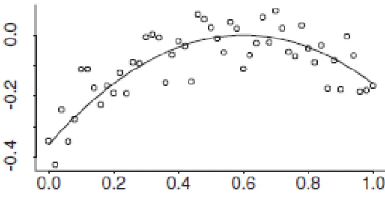
Consider the quadratic model shown in Figure 5:
21
Figure 5: Quadratic model
For the model (4.4), the corresponding basis functions are 1, x and x2 and the X-matrix is
.
Now, consider a different nonlinear data structure, called broken stick model. Figure 6 displays an example of the broken stick model. Points represent the data points and the line represents the model. As seen in the figure, two lines with different slopes join together at x = 0.6.
22
Figure 6: Broken stick model
Let us introduce a new basis function
to fit the broken stick model
(4.5)
Then the X-matrix becomes
.
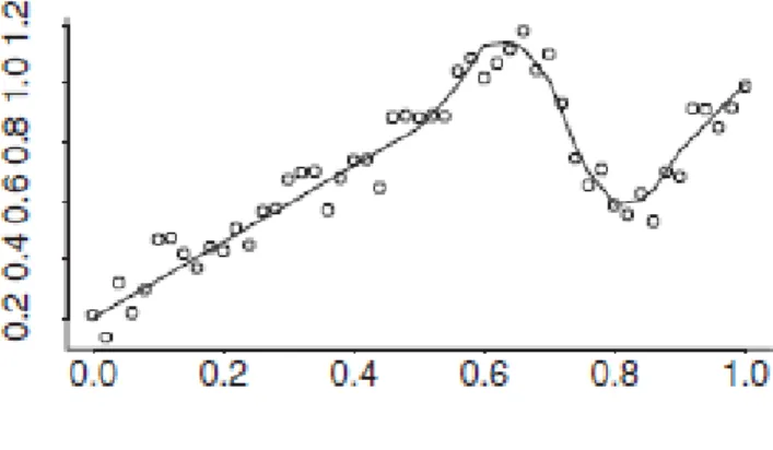
In real life, we may have more complex structures than the broken stick model. Figure 7 represents such a structure called whip model (Ruppert et al., 2003).
23
Figure 7: Whip model
We should introduce new basis functions of the form ( x – κ )+ , called a truncated
line,to handle this complicated structure. The whip model in Figure 7 can be fitted with X-matrix, .
In general, we can write
(4.6)
The value κ in ( x – κ )+ is called as knot. A function of the form ( x – κ )+ is
called a linear spline basis function, and collection of such functions is called a linear spline basis. A spline is a piecewise linear function which is linear combination of linear spline basis functions (Ruppert et al., 2003).
Use of splines for smoothing gives too much flexibility because many possible fits can be made by changing the number and locations of the knots. However, this
24
flexibility creates a model selection problem since there are many candidate models. While too many knots lead to an overfit, few knots may give a poor fit. In order to overcome those problems, automatic knot selection procedures were proposed in the literature. One of them is the stepwise selection method proposed by Smith (1982). It starts with a subset of full basis, and then adds basis functions having the largest absolute Rao statistics step by step until reaching the full basis. Then basis functions having the smallest absolute Wald statistics are deleted stepwise until reaching the minimal basis. At each step, model is fitted with the current basis and the GCV (generalized cross validation) value of the fit is recorded. The fit having the lowest GCV gives the final estimate. Another method to choose knots is Bayesian variable selection approach proposed by Smith and Kohn (1996). Although performance of these methods is good, they are very complicated in terms of application.
Penalized spline regression is another method that keeps all the knots while limiting their effects. Consider the general spline model with K knots,
,
where is determined by the least squares criterion and . In order to have a smooth fit, a constraint should be imposed on , and this constraint can be for some number C, which is easy to implement. Hence, the minimization problem is now
(4.7) The problem (4.7) can be written as
25
Min s.t. . (4.8)
where
. The Lagrange relaxation of the problem is
, (4.9) where λ is called the smoothing parameter. The solution of (4.9) is
, (4.10)
and the fitted values are
. (4.11)
See, e.g., Ruppert et al., pp. 65-66 (2003).
4.1.2 Linear Mixed Models
There are two types of explanatory variables: fixed effects and random effects. Generally, levels of the fixed effect variables are chosen by the researcher with the purpose of comparing the effect of levels. Fixed effects are constants and estimated from the data. A variable is a random effect if the effects of the levels of that variable can be viewed as being like a random sample from a population of effects. Random effects influence the variance of the response and manage the variance-covariance structure of the response. For example, if the relationship between age and weight is investigated on fifty children, age of the children is fixed effect variable, and child is the random effect variable since each child is a randomly chosen subject from the population.
26
Mixed-effect models (or mixed models) are the extension of regression models that incorporates random-effects. They are generally used for representing grouped, therefore correlated, data that come from observational studies with hierarchical structure or designed experiments with different spatial or temporal scales. Increased popularity of linear mixed models resulted in significant improvements in software packages, which provide the analysis of linear mixed models with R, S-PLUS and SAS.
Consider the following linear regression model:
, (4.12)
where is the vector of response variables, is the design matrix of explanatory variables, is the vector of regression coefficients, and is the vector of error terms. The least-squares estimator of is calculated as and errors are assumed to be normal with
The linear mixed model is the expanded version of the linear regression model (4.12) with the equation:
, (4.13)
where are the same as in the linear regression model, is the design matrix for random effects, , , , and .
27
We need to estimate and and predict . Let be the estimated effects of fixed treatments, and be the estimated differences between subgroups and the population mean. Then (4.13) can be written as linear model with correlated errors:
where . (4.14) Then . For given , we have
, (4.15)
and for given , we have
(4.16)
as the best linear unbiased predictors of and (Ruppert et al., 2003; Wand, 2002), respectively.
Note that (4.15) and (4.16) require the estimation of covariance matrices and . Maximum likelihood (ML) and restricted maximum likelihood (REML), that maximize a likelihood function calculated from elements of y that does not depend on β, are two main methods used for the estimation of and .
4.1.3 Penalized Splines and Linear Mixed Models
Speed (1991) shows that penalized splines can be fit as mixed models. Hence, splines can be considered as best linear unbiased predictors. Wand (2002) also uses the mixed model theory to fit splines, and he states that the software for mixed model analysis can be used for smoothing.
28 ,
where . Then
. (4.17)
Wand (2002) makes a modification to shrink to have a smooth fit and imposes
that
. (4.18)
This modification forces to obey the rules of normal probability distribution with zero mean.
Let us define and
and design matrices and
Then, equation (4.17) can be written as
,
), (4.19)
which is the linear mixed model formula in (4.13).
Solving the penalized least squares problem
29
with and penalty gives the best predictors and (Robinson, 1991). The solution is
, (4.21)
where and was defined in (4.8); see Wand 2002.
4.2 Experimental Procedure of Proposed Study
Advanced technology is used for the synthesis of nanoparticles to be used for targeted drug delivery and diagnostics. In this process, different qualities are added to the nanoparticle according to their purposes. Nanoparticles can be characterized in order them to target some specific cells. Therapeutic agents can be inserted in nanoparticles to treat cells. Their chemical structures may help the imaging and so they will be useful for diagnostics. These objectives cannot be achievable without the proper design of the nanoparticles. There are five main design parameters of nanoparticles that help them in fulfilling their functions: type, shape, size, surface charge and concentration of the NP solution.
The data set used in this study is obtained from in-vitro nanoparticle-cell interaction experiments conducted by the Nanomedicine & Advanced Technologies Research Center. Three types of NPs were used for the experiments: silica, polymethyl methacrylate (PMMA) and polylactic acid (PLA). All of those NPs were spherical. Silica and PMMA nanoparticles are produced in two different sizes; namely, with diameters of 50 and 100 nm. PLA nanoparticles are produced in 250
30
nm diameter. For each type and size of NP, two surface charges, positive and negative, are selected. NP solutions with two different concentrations, 0,001 mg/l and 0,01 mg/l, were prepared.
In those experiments, "3T3 Swiss albino Mouse Fibroblast" type of healthy cell set was used. Cells were incubated in a medium containing 10% FBS, 2 mm L-glutamine, 100 IU/ml penicillin and 100 mg/ml streptomycin at 37°C with 5% CO2. After incubation, proliferating cells in the culture flask were passaged using PBS and trypsin-EDTA solution. Then the cells incubated for 24 hours were counted and placed on 96-well cell culture plates. NP solutions are added to those plates.
Micromanipulation systems in the labs established as a ''clean room'' principle are used in the in-vitro NP-cell experiments. Spectrophotometric measurement methods, transmission electron microscopy (TEM), and confocal microscopy were used to examine NP-cell interactions and to get the data. Figure 8 shows an example of TEM micrographs of iron oxide and CPMV nanoparticles.
For Silica and PMMA NPs, there are 8 different configurations (50 or 100 nm size, positive or negatively charged, 0.001 or 0.01 mg/l concentration); for PLA NPs, there are 4 different configurations (250 nm size, positive or negatively charged, 0.001 or 0.01 mg/l concentration). Those lead to 20 different configurations of NPs in total. For each of 20 different configurations of NPs, the experiments are repeated six times. At 3, 6, 12, 24, 36 and 48 hours of incubation, the number of NPs removed from the environment was counted by washing the solution. The difference between
31
that number removed from the environment and the initial number of NPs subjected to the cells gives the number of the NPs attached on cell surface or penetrated into the cells. Then the cellular uptake rate was found by dividing that number by the initial number of the NPs subjected to the cells.
Figure 8: TEM micrographs of (a) iron oxide nanoparticles and (b) CPMV nanoparticle. The length of scale bar is 30 nm (Zhang et al., 2008)
For eight different configurations of Silica NPs, the experiments were repeated and measurements were taken at 1.5, 4, 9, 18, 30 and 42 hours of incubation in order to observe the process in time intervals of the first replication. For two configurations of PMMA NPs (size of 50 and 100 nm with concentration of 0.001 mg/l and positive surface charge), the experiments were repeated and measurements were taken at the same time points as those of the first replication to check for the consistency of the results of the first replication. The figures of raw data can be seen in Appendices A.1, A.2, and A.3 for Silica, PMMA, and PLA nanoparticles respectively.
32
Chapter 5
Proposed Model
In this study, we want to predict cellular uptake rate of NPs having different properties with respect to time. Therefore, we use penalized spline smoothing mixed effects model, which is explained in detail in Chapter 4. Moreover, we decided to use quadratic truncated line basis since it enables us to handle the apparent nonlinear structure of the raw data. We fit a model for each type of nanoparticle, Silica, PMMA, and PLA; because their interactions with cells are very different from each other. For example, the uptake rate of Silica NPs is more stable than that of PMMA nanoparticles, which means that the change in the ratio of the number of attached nanoparticles is less than those of PLA and PMMA nanoparticles.
Table 1 presents the NP characteristics used in our research.
In addition to the input variables of Table 1, a categorical random effect variable, Repeat, is defined to track the replication number for the models of Silica and PMMA. Repeat has two levels, 1 and 2, since the experiments were replicated twice for Silica and PMMA. It has no fixed effect counterpart. We may consider repeated experiments as randomly chosen subjects from a population. Since we do not want to make inference just for those two observed replications, and we want to
33
predict general behavior of the population for future replications, we include Repeat as a random effect.
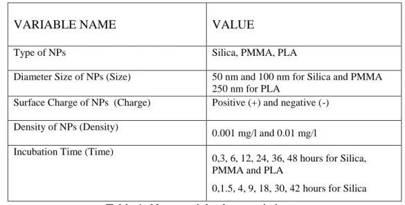
VARIABLE NAME VALUE
Type of NPs Silica, PMMA, PLA
Diameter Size of NPs (Size) 50 nm and 100 nm for Silica and PMMA 250 nm for PLA
Surface Charge of NPs (Charge) Positive (+) and negative (-) Density of NPs (Density)
0.001 mg/l and 0.01 mg/l Incubation Time (Time)
0,3, 6, 12, 24, 36, 48 hours for Silica, PMMA and PLA
0,1.5, 4, 9, 18, 30, 42 hours for Silica
Table 1: Nanoparticle characteristics
The aim of this study is to predict the cellular uptake rate. Hence, the cellular uptake rate is the output variable for all types of NPs. It is calculated according to formula
(5.1)
Detailed information about the data can be found in Section 4.2 in Chapter 4. In the Sections 5.1 - 5.3, the models for Silica, PMMA, and PLA nanoparticles will be explained, respectively. In those sections, fitting procedures are explained in three steps. In the first step, input variables and the design matrices of mixed models are defined. In the second step, the model is constructed. In the third step, the model parameters are estimated. Then prediction intervals are derived in Section 5.4 1st
34
5.1. Proposed Model for Silica Nanoparticles
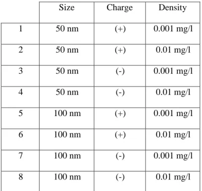
For Silica NP experiments, all possible combinations of input variables stated in Table 1 were used. The experiments were repeated twice with different incubation times. In the first replication, measurements were taken at 3, 6, 12, 24, 36, 48 hours of incubation. In the second replication, measurements were taken at 1.5, 4, 9, 18, 30, 42 hours of incubation. Hence, for each replication, there are 8 groups of nanoparticles. Table 2 presents those groups.
Size Charge Density
1 50 nm (+) 0.001 mg/l 2 50 nm (+) 0.01 mg/l 3 50 nm (-) 0.001 mg/l 4 50 nm (-) 0.01 mg/l 5 100 nm (+) 0.001 mg/l 6 100 nm (+) 0.01 mg/l 7 100 nm (-) 0.001 mg/l 8 100 nm (-) 0.01 mg/l
Table 2: Experimental groups of Silica and PMMA nanoparticles
Step 1: Setting up the input variables and design matrices
In this model, we want to predict the fraction of Silica NPs attached to cell
35
variables Size, Charge, Density; and the continuous variable, Time. Thus, input variables are Size, Charge, Density, and Time. Uptake rate (U) is the output variable. Furthermore, our model does not have intercept because uptake rate is zero at time zero. We also include the interactions between categorical variables and Time, and Time2 into the model since the design matrix of the quadratic
spline basis is as explained in Chapter 4. Then design matrix consists of the fixed effect variables Time (T), Time×Size (TS), Time×Charge
(TC), Time×Density (TD), Time×Size×Charge (TSC),
Time×Size×Density (TSD), Time×Charge×Density (TCD),
Time×Size×Charge×Density (TSCD), Time2 (T2), Time2×Size (T2S),
Time2×Charge (T2C), Time2×Density (T2D), Time2×Size×Charge
(T2SC), Time2×Size×Density (T2SD), Time2×Charge×Density (T2CD) and Time2×Size×Charge×Density (T2SCD).
Recall that our mixed effects model formulation in (4.13) was
.
Hence, the design matrix becomes
. (5.2)
To construct Z-matrix, firstly we need to choose the places for the knots. The number of knots affects the size of the model. A large number of knots increase the
36
number of parameters to be estimated and the computation time while too few knots lead to a poor fit.
Ruppert et al. (2003) propose that the number of knots should be
(5.3)
and the knot locations should be
for k=1,..,K. (5.4)
Those formulas generally give good results but sometimes adjustments are required.
We have 12 unique Time values. Hence, required number of knots is found three with formula (5.3) and knot locations are calculated as κ1 = 5.5, κ2 = 15 and κ3
= 31.5 by (5.4). Thus, the quadratic spline basis for our model becomes
(5.5)
We build a model which includes random counterparts of all the fixed effect variables. Hence, the Z-matrix becomes
37
. (5.6)
We fit our model to the data by using lme() function of package nlme in software R. Firstly, we build a model with X and Z matrices defined in (5.2) and (5.6), respectively, to consider all possible fixed and random effect variables. Then we test for the significance of terms and eliminate insignificant ones. In order to test the significance of the terms, we fit a model with and without a given term. Then we apply ANOVA. If p-value is less than 0.05, then we keep that term in the model. Otherwise, we eliminate it. Moreover, Repeat (R) is modeled as a random effect because we want to make inference not only for those two replications but also for the future replications.
According to the test results, we find that Time (T), Time×Size (TS), Time×Charge (TC), Time×Density (TD), Time×Size×Charge (TSC), Time×Charge×Density (TCD), Time2 (T2), Time2×Size (T2S),
Time2×Charge (T2C), Time2×Density (T2D), Time2×Size×Charge
(T2SC), Time2×Charge×Density (T2CD), and
Time2×Size×Charge×Density (T2SCD) are statistically significant fixed effect variables. Time2×Size×Density (T2SD), Time×Size×Density (TSD), and Time×Size×Charge×Density (TSCD) are insignificant fixed effect
38
variables with p-values 0.0823, 0.9786, and 0.424, respectively. Random effect counterpart of Size and Size×Density turns out to be insignificant with p-values 0.1805 and 0.9999 respectively. Hence, after the elimination of insignificant terms, the final design matrices are
, (5.7) and . (5.8)
Step 2: Model formulation
For Silica NPs, the proposed model is
(5.9) where all f functions are smooth functions of the terms whose both fixed and random counterparts are statistically significant .
39
With the mixed model formulation, (5.9) is written as
(5.10)
where are fixed parameters and are random
variables for replications 1 and 2, respectively, where k=1, 2, 3.
Step 3: Estimation of model parameters
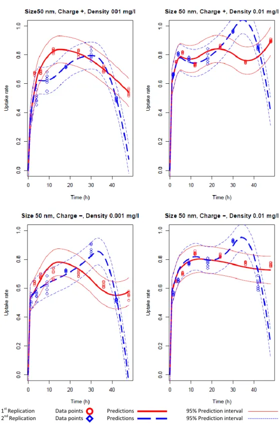
The model (5.10) is implemented in R using lme() function in the nlme package (see Appendix B.1 for the code). Then and are obtained. To see the hourly predictions of the cellular uptake, X and Z matrices are formed for hourly grid Time=0,1,…49 hours. Using those matrices, the fitted lines are obtained with the formula
. (5.11)
40
1st Replication Data points Predictions 95% Prediction interval 2nd Replication Data points Predictions 95% Prediction interval
41
1st Replication Data points Predictions 95% Prediction interval 2nd Replication Data points Predictions 95% Prediction interval
42
5.2. Proposed Model for PMMA Nanoparticles
For PMMA NP experiments, the same eight combinations of input variables of Table 2 were used. The measurements were taken at 3, 6, 12, 24, 36, 48 hours of incubation. The experiments were repeated for positively charged nanoparticles with concentration of 0.001 mg/l. Measurements were taken at the same time points with the previous replication to be sure of the results since PMMA NPs having those characteristics behave different from the other configurations of PMMA NPs.
Step 1: Setting up the input variables and design matrices
In this model, we want to predict the fraction of PMMA NPs attached to cell surface or penetrated into the cell. Input variables are two level categorical variables, Size, Charge, and Density; and the continuous variable, Time. Intercept is forced to be zero because uptake rate is zero at time zero. Hence, we do not have intercept term, and involve the interactions between the categorical variables and Time, and Time2. Uptake rate (U) is the output variable.
Initially, all the terms and their interactions mentioned above are added to the model as both fixed and random effects. Then design matrix consists of the fixed effect variables Time (T), Time×Size (TS), Time×Charge (TC), Time×Density (TD), Time×Size×Charge (TSC), Time×Size×Density (TSD), Time×Charge×Density (TCD), Time×Size×Charge×Density (TSCD), Time2 (T2), Time2×Size (T2S), Time2×Charge (T2C),
43
Time2×Size×Density (T2SD), Time2×Charge×Density (T2CD) and Time2×Size×Charge×Density (T2SCD). Hence, it becomes
. (5.12)
We have 12 unique Time values in PMMA NP experiments, and 3 knots are recommended by (5.3). However, a poor fit is obtained with 3 knots, whose locations are computed by (5.4). We tried 5 knots which give a more satisfactory fit. Knots are located at κ1 = 5.5, κ2 = 10, κ3 = 18, κ4 = 28 and κ5 = 38 by (5.4). Quadratic spline
basis becomes
, (5.13)
and Z matrix becomes
44
. (5.14)
Moreover, Repeat (R) is modeled as a random effect as in the model of Silica NPs.
Firstly, we fit a model with X and Z matrices in (5.12) and (5.14), respectively. Then we apply ANOVA to test the significance of each term in the model. We find that Time (T), Time×Size (TS), Time×Charge (TC), Time×Density (TD), Time×Size×Charge (TSC), Time×Size×Density (TSD), Time×Charge×Density (TCD),Time×Size×Charge×Density (TSCD) and Time2 (T2) are the significant fixed effect variables since p-values are less than 0.002.
After removing the statistically insignificant variables, the new X and Z matrices become , (5.15) and
45 , (5.16) respectively.
Step 2: Model formulation
For PMMA NPs, the proposed model is
(5.17)
where all f functions are smooth functions. The final mixed model can now be written as
(5.18)
where are fixed effects and are random effects
46
Step 3: Estimation of model parameters
The R code for the implementation of model (5.17) can be seen in Appendix B.2. Using the values and obtained from R, the fitted lines for replication 1 and 2 are calculated by (5.8) for hours 0 to 48 with the appropriate X and Z matrices formed for hourly grid Time= 0, 1,..,49 hours. Hourly predictions for PMMA NPs can be seen in Figure 11 and 12.
47
1st Replication Data points Predictions 95% Prediction interval 2nd Replication Data points Predictions 95% Prediction interval
48
1st Replication Data points Predictions 95% Prediction interval 2nd Replication Data points Predictions 95% Prediction interval
49
5.3. Proposed Model for PLA Nanoparticles
In PLA experiments, nanoparticles of 250 nm size were used only because of technical feasibility of synthesizing. Measurements were taken at 3, 6, 12, 24, 36, 48 hours of incubation.
Size Charge Density
1 250 nm (+) 0.001 mg/l
2 250 nm (+) 0.01 mg/l
3 250 nm (-) 0.001 mg/l
4 250 nm (-) 0.01 mg/l
Table 3: Experimental groups of PLA nanoparticles
Step 1: Setting up the input variables and design matrices
In this model, we want to predict the fraction of PLA NPs adhered on the cell surface or penetrated into the cell. Input variables are two level categorical variables, Charge and Density; and the continuous variable, Time. Size is not an input variable here because it has only one level. Intercept is zero since the uptake rate is zero at time zero, as mentioned before for Silica and PMMA. Moreover, we involve the interactions between categorical variables and Time, and Time2. Uptake
rate (U) is the output variable.
Initially, all the terms and their interactions are added to the model as both fixed and random effects. Then the design matrix becomes
50
(5.19)
We obtain a good fit with 3 knots. Knots are located at κ1 = 7.5, κ2 = 18 and κ3
= 33 by (5.4). The quadratic spline basis for our model becomes
. (5.20)
Then the Z-matrix becomes
(5.21)
After fitting our model to the data, we test the significance of each term in X and Z matrices via ANOVA and eliminate insignificant ones. According to the test results, we find that Time (T), Time×Charge (TC), and Time2 (T2) are significant fixed effect variables with p-values less than 0.0001. Their random counterparts are also significant. After eliminating the insignificant terms, the new X and Z matrices become
(5.22)
and
51
(5.23) respectively.
Step 2: Model formulation
For PLA NPs, the new model becomes
, (5.24)
where is a smooth function of Time and is a smooth function of Time×Charge (TC). The final mixed model formulation becomes
(5.25)
where are fixed coefficients, and are random coefficients
where
Step 3: Estimation of model parameters
The model (5.25) is implemented in R with the code in Appendix B.3. Then the values and are acquired from R, and the predictions are calculated by (5.8) for hours 0 to 48 with the appropriate design matrices. Figure 13 displays both data and fit from our model.
52
1st Replication Data points Predictions 95% Prediction interval
53
5.4. Derivation of Prediction Intervals
The aim of this research is to predict NP-cell interaction based on results of the experiments conducted with Silica, PMMA, and PLA NPs. Hence, we want to know the interval in which our future estimates will fall. Therefore, we need to find prediction intervals.
Recall the mixed model formulation in (4.13)
,
where . We can write
, (5.26)
where and . For the mixed model representation of penalized splines, Ruppert et al. (2003) derive the 100(1-α)% confidence interval as
(5.27)
where
, (5.28)
, and . Therefore, 100(1-α)% prediction interval for our case is
54
Figures 9-13 plot both the fits and their 95% prediction intervals obtained from our models.
55
Chapter 6
Comparison and Discussion
In this thesis, cellular uptake of nanoparticles is investigated through a mixed model. Mixed models are formed by extending regression models with random effects. As explained in Chapter 4, mixed models handle semiparametric smoothing since smoothing methods that utilizes basis functions with penalization can be represented as a mixed model. They are generally preferred for clustered, hence dependent, data collected hierarchically. This situation arises, for example, when observations are obtained from related subjects or when data is collected on the same subject over time.
In our study, we model the uptake rates of Silica, PMMA, and PLA nanoparticles into the cell in 48-hour time interval by means of a penalized moothing splines mixed effects model. For each type of NP (Silica, PMMA, and PLA), we develop a model that takes NP size, charge, concentration and incubation time as inputs to predict the cellular uptake rate. For Silica NP experiments, the experiments are repeated for all eight groups of different size, charge, and solution concentration. Observations are taken at different time points in two replications. Also, for PMMA NPs, the experiments conducted with positively charged NP solutions of 0.001 mg/l