Capacity of noisy, discrete memoryless channels under input constraints

■ ■ С А Р Ж !Τ Υ ' O r ; н а ш , ,

S lS S B iT ë ' MfcMOñYLÉSS, о

'U M O iiR · O O 'N 'S T BaIMTS'·^· ■ « i W -Ѣ ■ :■*' ·; ‘ *W· '*· '■ ■ -. . O' о i İT. J V · —· A-· ¿ г ; Γϋ' I’ '^Л. 1·· ' Г -·; ·■.■ ·■« ' ■ "'jW..· Γ.'··,.·,·η ^ . . ,

Qf9

Ζ6Ψ

. Ä 3 ? t

/330

C A P A C IT Y OF N O IS Y ,

D IS C R E T E M E M O R Y L E SS C H A N N E L S

U N D E R I N P U T C O N S T R A IN T S

A THESIS

SUBMITTED TO THE DEPARTMENT OF ELECTRICAL AND ELECTRONICS ENGINEERING

AND THE INSTITUTE OF ENGINEERING AND SCIENCES OF BILKENT UNIVERSITY

IN PARTIAL FULFILLMENT OF THE REQUIREMENTS FOR THE DEGREE OF

MASTER OF SCIENCE

tarafiadan l)2|5o!aami§iir.

By

Ezhan Kara§an June 1990

I certify th at I have read this thesis and th at, in my opinion, it is fully adequate, in scope and in quality, as a thesis for the degree of Master of Science.

Associate Prof. Dr. Erdal Arikan (Principal Advisor)

I certify th a t I have read this thesis and th at, in my opinion, it is fully adequate, in scope and in quality, as a thesis for the degree of Master of Science.

Associate Prof. Dr. Melek D. Yücel

I certify th at I have read this thesis and th at, in my opinion, it is fully adequate, in scope and in quality, as a thesis for the degree of Master of Science.

T

A s s i.s ta n t Prof. Dr. Gürhan Şaplakoğlu

Approved for the J^istitute of Engineering and Sciences:

f _____________

Prof. Dr. M ehm etB aray

A B S T R A C T

In this thesis work, we examine the capacity of discrete memoryless channels under input constraints. We consider a certain class of input-restricted channels for which con­ strained sequences can be modeled as outputs of a finite-state machine(FSM). No efficient algorithm is known for computing the capacity of such a channel. For the noiseless case, i.e., when the channel input letter and the corresponding output letter are identical, it is shown th at [1] the channel capacity is the logarithm of the largest eigenvalue of the adjacency m atrix of the state-transition diagram of the FSM generating the allowed chan­ nel input sequences. Furthermore, the probability distribution on the input sequences achieving the channel capacity is first-order markovian.

Here, we discuss the noisy case. For a specific input-restricted channel, we show that unlike the noiseless case, the capacity is no longer achieved by a first-order distribution. We derive upper and lower bounds on the maximum rate achievable by a K-th order markovian distribution on the allowed input sequences. The computational results show that the second-order distribution does strictly better than the first-order distribution for this particular channel.

A sequence of upper bounds on the capacity of an input-restricted channel is also given. We show that this sequence converges to the channel capacity. The numerical results clarify that markovian distribution may achieve rates close to the capacity for the channel considered in this work.

Keywords: Channel capacity. Input-restricted channel, Finite-state machine, Marko­ vian distribution.

Ö ZET

Bu tez çalışmasında girdi kısıtlamaları altında ayırtık, hafızasız kanalların sığaları İncelenmektedir. Burada tartışılan girdi kısıtlamak kanallar için izin verilen girdi dizileri bir sonlu durumlu makinenin çıktıları olarak modellenebilir. Böyle bir kanalın sığasını hesaplayabilmek için verimli bir algoritma bilinmemektedir. Gürültüsüz durumda (kanal girdi harfiyle karşılık gelen çıktı harfi aynı olduğu zaman), Shannon[l] kanal sığasının, kısıtlandırılmış kanal girdi dizilerini üreten sonlu durumlu makinenin bitişiklik matrisinin en büyük özdeğerinin logaritm asına eşit olduğunu göstermiştir. Ayrıca, kanal sığasına ulaşan girdi dizileri üzerindeki olasılık dağılımı birinci dereceden bir markov dağılımıdır.

Bu çalışmada biz gürültülü durumu tartışıyoruz. Belirli bir girdi kısıtlamak kanal için, gürültüsüz durumdan farklı olarak, sığanın birinci dereceden bir markov dağılımı tarafından ulaşılamadığı gösterilmektedir. İzin verilen girdi dizileri üzerinde K ’nıncı derece­ den bir markov dağılımının ulaşabileceği en yüksek hız üzerine alt ve üst sınırlar elde edilmektedir. Hesaplamalar sonucunda ikinci dereceden bir dağılımın birinci dereceden bir dağılıma göre daha yüksek hızlara ulattığı görülmüştür.

Bu çalışmada ayrıca girdi kısıtlamak kanalların sığaları üzerine bir üst sınırlar dizisi verilmektedir. Bu dizinin kanal sığasına yakınsadığı gösterilmektedir. Hesaplamalar sonu­ cunda bu çalışmada kullanılan kanallar için markov dağılımlarının kanal sığasına oldukça yakın hızlara ulaştıkları gözlenmektedir.

Anahtar sözcükler: Kanal sığası. Girdi kısıtlamak kanal. Sonlu durumlu makine, Markov dağılımı.

A C K N O W L E D G E M E N T

I would like to express my gratitutes to Dr. Erdal Arikan, my supervisor, for his invaluable guidance and suggestions throughout this work. I also thank to N. Gem Oğuz and M. Şenol Toygar for their helps in drawing the figures in the thesis. Special thanks are due to Oya Ekin for her moral support and help in typewriting the text.

Contents

1 IN T R O D U C T IO N 1

1.1 Examples of Input-Restricted Channels 2

1.2 Capacity of Input-Restricted DMC’s ... 3 1.3 Com putation of Channel C a p a c i t y ... 4 1.4 Capacity of Input-Restricted ChannelsiThe Noiseless C a s e ... 5 1.5 Probability Assignments on Constrained Sequences and Summary of Results 5

2 C A P A C I T Y OF N O ISY , IN P U T C O N ST R A IN E D C H A N N E L S 8

2.1 Upper and Lower Bounds on the Maximum Rate Achievable by Markovian D is trib u tio n ... 8 2.2 Com putational R e s u lts ... 11

2.3 Upper bounds on C 13

2.4 Rate of Convergence of Cyv to the C a p a c ity ... ... . . 15

3 C O N C L U SIO N S 20

A Proof that the limit in (1.1) exists 21

B List of Upper Bounds on the Capacity 23

R E F E R E N C E S

List of Figures

1.1 State-transition diagram for an input constraint

1.2 State transition diagram for RLL(d,k) c o d e ... 3 1.3 State transition diagram for charge c o n s tr a in t... 3 1.4 Double-step transition diagram for the channel constraint in Figure 1.1 . . . 6

2.1 Cn vs. N for constrained BSC with e= 0 . 0 1 ... 17

2.2 Cn vs. N for constrained BSC with e = 0 . 0 5 ... 17

2.3 Cn vs. N for constrained BSC with e= 0.1 18

2.4 Catvs. N for constrained BEC with e=0.1 18

2.5 Catvs. N for constrained BEC with e= 0.2 19

2.6 Catvs. N for constrained BEC with e=0.3 19

List of Tables

2.1 Computed bounds for BSC 1.3

2.2 Computed bounds for B E C ... 13 2.3 Upper bounds computed by Arimoto-Blahut algorithm(BSC) 14 2.4 Upper bounds computed by Arimoto-Blahut algorithm(BEC) 14

B .l Upper bounds computed by Arimoto-Blahut a lg o rith m (B S C )... 23 B.2 Upper bounds computed by Arimoto-Blahut a lg o rith m (B S C )... 24 B.3 Upper bounds computed by Arimoto-Blahut a lg o rith m (B S C )...24 B.4 Upper bounds computed by Arimoto-Blahut a lg o rith m (B E C )...2-5

C hapter 1

IN T R O D U C T IO N

In this ^thesis work, we examine the capacity of discrete channels for which input sequences are restricted to satisfy certain channel input constraints. To introduce the problem, consider a binary symmetric channel

(BvSC)

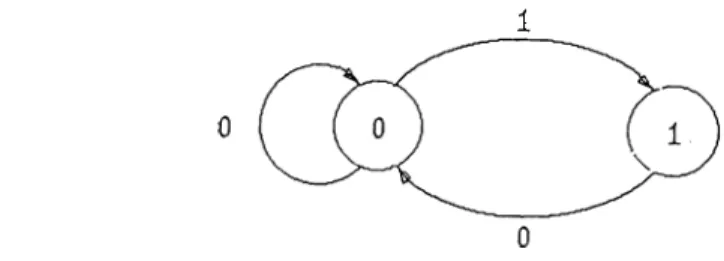
with the restriction th at input sequences cannot contain consecutive I ’s. For example, the sequence (1 ,0 ,0 ,0 ,1 ,0 ,1 ,0 ,0 ,1 ,0 ) is an allowed input sequence, whereas (1 ,0 ,1 ,1 ,0 ,0 ) is not. These constraints can be presented by the finite-state machine (FSM) in Fig. 1.1. The binary numbers assigned to each state transition corresponds to the output of the FSM produced on th at transition. It is readily seen th a t no sequence of transitions will generate a sequence containing consecutive I's.

Figure 1.1: State-transition diagram for an input constraint

There is no known practical algorithm for computing the capacity of an input- restricted channel. Even for the simple channel with an input constraint represented by the FSM in Fig.1.1, the capacity is unknown. The difficulty is caused by the input constraints on the one hand and the noisy nature of the channel on the other. Although the channel is memoryless, each letter at the channel output depends on the corresponding input and on the past input and output letters. An efficient way for computing the capacity is presently unknown.

input distributions. We show th at, unlike the noiseless case for input- restricted channels, improvements in the achievable rate are obtained by increasing the memory of markov distribution. We present numerical results for the channel in Fig. 1.1 showing this im­ provement. We also derive upper bounds on the channel capacity to see how close one can get to capacity by using markovian channel input distributions.

In the rest of this introductory chapter, we define the above concepts more precisely, state the problem and give a summary of results. In section 1.1, we give examples of channel constraints that find various applications in practice. In section 1.2, we define the capacity of input-restricted, discrete, memoryless channels and give a brief review of channel coding theorem. Computation of the capacity of a discrete constrained channel is discussed in section 1.3. In section 1.4, we summarize the earlier work of Shannon [1] on the capacity of discrete, input-restricted, noiseless channels and on the input distribution achieving capacity. In the final section, we introduce markovian distributions on the allowed input sequences and the main contribution of this thesis is stated.

CHAPTER 1. INTRODUCTION

2

1.1

E xam p les o f In p u t-R e str ic te d C h an nels

In this section, we give two examples of input-restricted channels and explain the state diagram presentation of such channels. Both examples presented here belong to the class of input-restricted channels for which the allowed input sequences can be modeled as outputs of a FSM, with a set of states S = {^i, 5*2, . . . , S j } and at each state transition a letter from a discrete alphabet A is produced. Throughout this work, we consider input-restricted channels where constrained sequences are generated by FSM ’s.

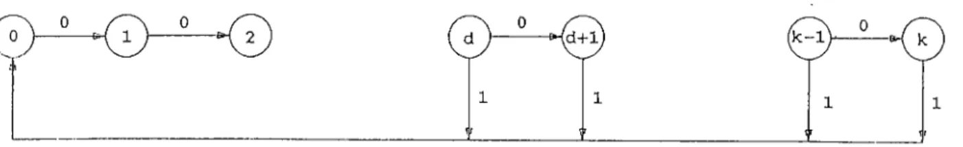
Input-restricted channels play an im portant role in many digital transmission and recording systems, such as magnetic recording and optical transmission and recording. Recording codes based on runlength-limited sequences are widely used in optical and magnetic disk recording applications. In digital magnetic recording systems, encoding schemes (such as NRZI) encode a 1 by a change in the magnetization polarity and a 0 by no change in polarity. Systems using self-clocking for clock regeneration require frequent changes in polarity. Long sequences of like polarity may result in loss of synchronization. Therefore, the encoded sequences are restricted by design to have a maximum runlength (k-f-1), i.e., the number of consecutive O’s between any two I ’s does not exceed k. A second type of constraint is imposed by the intersymbol interference considerations. In order to reduce intersymbol interference, a constraint is placed on the minimum number of O’s between neighboring I ’s which is denoted by d; (d + 1) is called the minimum runlength of the code. The resulting code with parameters (d,k) is called a runlength limited (RLL) code. RLL(d,k) sequences may be thought as being generated by a finite-state machine with state transition diagram given in Fig. 1.2.

CHAPTER 1. INTRODUCTION

0 - ^ * 0

Figure 1.2: State transition diagram for llLL(d,k) code

The input-restricted channel in Fig. 1.1 corresponds to a runlength constraint (l,oo) on the input sequences.

Another kind of restriction on binary sequences is the charge constraint. Charge constrained sequences with maximum charge C are generated by an FSM with (2C+1) states as shown in Fig. 1.3.

( - C + 1 I

0

Figure 1.3: State transition diagram for charge constraint

1.2

C ap acity o f I n p u t-R e s tr ic te d D M C ’s

Consider a discrete memoryless channel (DMC), with input alphabet A , output alphabet B and channel transition probabilities P{y\x)^ y E B^ x E A. Let Ayv be the set of channel input sequences = ( x i , . . , ,xj\j) ^ X{ E A , i = 1, . . . , A , of length N th a t satisfy the channel input constraints, starting from an arbitrary state(initial state not fixed).

The capacity C, of such a channel is defined by: C = lim sup — — —

-Pn(Xt^) A'

(1.1)

where Pn{·) is a probability distribution on Ayv, I { X ^ ; Y ^ ) is the average mutual infor­ mation between channel input sequence and channel output sequence

Pn( Y ^ \ X ^ )

/ ( X ^ ; F ^ ) = X ; P N { Y ^ \ X ^ ) P N i X ^ ) \ o g

CHAPTER 1. INTRODUCTION

and

N

¿=1

since the channel is memoryless. The proof of the existence of the limit in (1.1) is given in Appendix A.

The channel capacity is a quantity of information theoretical significance [1]: At rates below it, we can communicate reliably through the channel by choosing proper encoding and decoding strategies (the term reliably means that, the probability of error averaged over the ensemble of codes can be made arbitrarily close to zero). Conversely, for rates exceeding the capacity, the probability of error for any encoder-decoder pair is bounded away from zero.

Determining channel capacity requires finding the probability distribution th at max­ imizes the average m utual information. Knowledge of this probability distribution is also valuable in the construction of actual encoders and decoders.

1.3

C o m p u ta tio n o f C h an nel C ap acity

The computation of channel capacity is a maximization of a nonlinear function over many variables with equality and inequality constraints. Fortunately, this problem is greatly simplified by the convexity of the average mutual information function, and there exists an algorithm for finding the capacity of a DMC (without input constraints) devised by Arimoto [4] and Blahut [5]. Starting from an arbitrary input distribution, the algorithm converges to the capacity.

When constraints on channel input sequences exist, making use of the Arimoto- Blahut algorithm we can compute

1

Cn = -Tt I { X ^ \ Y ^ )

for any fixed N > 1, by considering the extended channel with input alphabet Ayv ^nd channel transition probabilities

However, we have no efficient way of computing the capacity C = lim 6V· Though TV—^oo

it is possible in principle to approximate C as closely as desired by computing Cm for N sufficiently large, this quickly becomes impractical since the com putation complexity grows exponentially in N. If we stop at a certain iV, we have an upperbound on C, given by C < Cm as stated in Appendix A.

1.4

C a p a city o f In p u t-R e str ic te d C h a n n els:T h e N o iseless

C ase

CHAPTER 1. INTRODUCTION

5

Suppose th at we transm it the constrained sequences through a noiseless channel, i.e., the channel input letter and the corresponding output letter are identical. In this case, the probability distribution on the constrained channel input sequences achieving the capacity is first-order markovian, as shown by Shannon [1, Theorem 8]. That is, no improvement in maximum rate is possible by considering higher order distributions. Also, a formula is given in [1] for computing the capacity in the noiseless case:

C = log IT

where W is the largest eigenvalue of the adjacency m atrix of the state transition diagram of the FSM [1, Theorem 1]. In fact. Shannon’s result covers the case where letters may have different time durations.

In this work, we are concerned with the noisy, input-restricted DMC’s and we ask whether the capacity is still achieved by a first-order markovian distribution on the con­ strained input sequences. Before discussing this problem, we will consider markovian distributions on the constrained input sequences th a t are generated by a FSM.

1.5

P r o b a b ility A ssig n m en ts on C o n stra in ed S eq u en ces and

S um m ary o f R e su lts

In section 1.1, examples of constraints where allowed channel input sequences can be represented as outputs of a FSM were presented. Suppose we have a FSM with a set of states S = {*?!, ¿'25 · · · i and at each time instant, a state transition occurs and a letter from a discrete alphabet A is produced.

The probability distribution on the constrained sequences is first-order markovian if P r { a ; t + i |5 < , S ( _ i , . = P r{ x i+ i|5 i) (1.2) all St E Xt^i E: A ^ t Ei Z ( Z is the set of integers, where St is the state of the machine at time t and Xt^i is the output produced at time ( t + 1)).

If probabilities {pij} are assigned to the transition from state S{ to state with

J

Pij > 0, y^jHj = 1 all z = 1 , 2 ,..., J , then the probability of the letter emitted at any time i=i

instant depends only on the previous state and the distribution on the allowed sequences will be first-order markovian.

CHAPTER 1. INTRODUCTION

6

We can also consider a K-th order markovian distribution on the channel input sequences so th at each produced letter depends statistically only on the K previous states.

P r { x t + l \ s t , S t - l

=

P r { X t + l \ S t , S t - l

, . . . ,

S t - K + l }

One can view the K-th order Markov distribution for a FSM as a one-step Markov distribution for an extended FSM, which also models the same input constraints. For a given FSM, consider the possible state sequences of length K and construct a new FSM with each state corresponding to to such a sequence. Let 5 ' =

represent the state space of the new FSM, where S- = (Si^^ ^ 1 < ik < J· Assign an edge from .S'^ = (S'q, Si^, . . . , Si,^) to 5'· = {Sj, Sj,^.) if Sj^ = 5,·,^^, I = l , . . . , ( / i " — 1) and the letter emitted at th at transition is the letter produced at the transition from Sij^^ to Si,. in the original FSM.

If a first-order markovian distribution is defined on the sequences generated by the new FSM, then by (1.2),

= P r{a;i+ i|s'J

= |s ij, . . . , }

where s[ = , · . . , Stj^) £ 5" and 5^. E *?, i = 1 , . . . , /if. The sets of sequences generated by both machines are identical. Hence, we obtain a K-th order markovian distribution on the sequences generated by the original FSM.

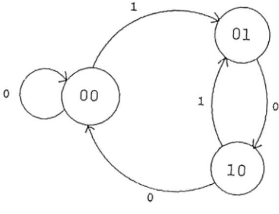
As an illustration, a two-step transition diagram for the channel constraint given in Figure 1.1 is shown in Figure 1.4. The set of states S = {.?o — (00),i?i = (01), ^2 = (10)}

Figure 1.4: Double-step transition diagram for the channel constraint in Figure 1.1 includes all possible state sequences of length two th at can be generated by the FSM in Figure 1.1. Letters produced at each state transition are assigned as labels to the edges. If we assign non-negative probabilities {pij} on each directed branch with poo + Poi =

1 i Pi2 = 1 i P21 + P20 = 1) then the distribution on the sequences generated by the FSM in Fig. 1.4 will be first-order markovian which corresponds to a second-order distribution on the sequences generated by the FSM in Fig. 1.1.

Note that the set of first-order markovian probability distributions on the con­ strained sequences is a subset of the set of second order distributions.

Our main contribution in this context is an answer to the question mentioned in section 1.4 stating that the input distribution maximizing the average mutual information is not first-order markovian. In particular, our lower and upper bounds on the maximum rate achievable by markovian input distribution show that using a second-order markovian distribution on the allowed input sequences for the input-restricted BSC for which con­ strained sequences are generated by the FSM in Fig. 1.1, higher rates can be achieved as compared with the first-order distribution. Hence, assuming a markovian distribution on the constrained input sequences of a noisy channel, we may achieve higher rates by con­ sidering higher order markovian distributions. Using the observation made in section 1.5, we may believe that second-order markovian distribution also does not achieve capacity, since it can be viewed as a first-order distribution for another FSM.

CHAPTER 1. INTRODUCTION

7

In the next chapter, our main results are presented and discussed. In chapter 3, conclusions and suggestions for future research are stated.

C hapter 2

C A P A C IT Y OF N O ISY ,

IN P U T -C O N S T R A IN E D C H A N N E L S

In section 2.1, upper and lower bounds on the maximum mutual information achieved by markovian input distribution are derived. The results obtained by using these bounds on the capacity of binary symmetric channel (BSC) and binary erasure channel (ВЕС) with the input constraint given in Fig.1.1 are tabulated and discussed in section 2.2. In section 2.3, the upper bounds Cm computed by using Arimoto-Blahut algorithm for the same channels are given both tabularly and graphically. In the final section, a new problem dealing with the convergence in the capacity is discussed.

2.1

U p p er and Low er B o u n d s on th e M axim u m R a te A ch iev ­

able by M arkovian D istr ib u tio n

By (1.1), the capacity of an iiTput-restricted, discrete channel is given by C = lim

N-^oo_Psup

n(X^ N

where for each A , the supremum is taken over all distributions on the con­ strained channel input sequences of length N. Since the set of such distributions on the constraint set is compact and the average mutual information function is continuous in Pat(X ^ ) , the supremum in (1.1) can be replaced by maximum [6, p.49].

In this work, we ask whether a first order markovian distribution achieves C . The results clarify that it does not. We prove this by showing that for the channel in Fig.1.1, a second order markovian distribution does strictly better than a first order markovian distribution. We define

CHAPTER 2. CAPACITY OF NOISY, INPUT CONSTRAINED CHANNELS

9

where the maximum is taken over all K-th order markovian distributions on the constrained channel input sequences th a t are generated by a FSM. In particular, we will show that Ri < R2 for the channel of Fig. 1.1.

To show this, we derive upper and lower bounds on R¡^. Assume th at the channel input distribution is stationary (when constrained input sequences are generated by a FSM with an irreducible and aperiodic set of states and the probability distribution on the sequences is markovian, then starting infinitely far in the past, the distribution becomes stationary since ergodicity implies the existence of limiting state probability distribution). When the channel input distribution is stationary,

Ti-\-k P i V n — Pn·) · · · ) Vn+k — /^n+A:) — ^ ^ · · · í ^n-\-k ~ ^ ’n+/c) P ^ V i — P i \ ^ i — ^'t) i = n k — ^ ^ P { ^ 0 — Í ^ k — ^ n - f A;) J[ P ( . y i ~ Pn-\-i — ^ n + i ) i= 0 ~ P { y O ^ P u ) · · · ^yk — Pn-\-k)

for all integers n, k and channel output sequences (/?n, · · · ^Pn-\-k) of length {k + 1), where the second equality is obtained by using the stationarity of the input distribution and the discrete memoryless channel assumption. Therefore, the channel output distribution is also stationary.

We can write

K^XN.^yN) ^

Define Hoo(Y) as lim ^ and by Theorem 3.5.1 of [2] ^ 7V-.CO N

Hoo{Y) = lim H( Yn\Yn-i, . . . , Yi)

N—*■00 (2.2)

On the other hand,

H{Y^\X^)

N

N

^ E { l o g p ^ ( ^ Y N \ X N y ^ } = Í E ^ í ( y n \ X n )X

(2.3) where the second equality follows since the channel is memoryless.

1

H ( Y n \ X n ) =

E

í ’Í!'" = = “ № » = « ) log ^ _

aeA,peB ~

Since the input distribution is stationary, for any n

CHAPTER 2. CAPACITY OF NOISY, INPUT CONSTRAINED CHANNELS

10

and since the channel is memoryless

P{yn = P\Xn

= a) =

P{y = P\x = a)

(2.5)

Then, by using (2.4) and (2.5), we obtain

H { Y ^ \ X ^ ) = N H { Y \ X ) where H { Y \ X ) is given by

n{Y\X) = J : P {

v

=

/J|x

=

a)P(x

=

CX j(3 (2.6) (2.7) By (2.2) and (2.6), (2.1) becomes Rk = Jim max f J i( r y y iy ;v _ a ,...,T i) - //( F |X ) ] N-^ooPj^(XN)

= lim max [7i (T o ii- i, · · ·, Y -n) - H{Yo\Xo)]

N-*oo

where the second equality follows from the stationarity of the channel output.

(

2

.

8

)

P r o p o s itio n 1 The maximum rate achievable by a K-th order markovian distribution on the input sequences of an input-restricted channel satisfies

(i) Rk < max f/7 (y o |y _ i,. . . ,y _ (N -i)) - 77(5"o|Xo)] Pn{X^)

(it) Rk > ^ m ax^^^^[/f(yo|y_i,. . . ,y_(£,_i),X _i,,. . . ,X_(L4-/c_i)) - //(YblvYo)] where the maximums are taken over all K-th order markovian probability distributions on the allowed input sequences.

P ro o f:

(i)

^max^^[ir(yo|y_i,... ,y_(N-i)) -

H{Yo\Xo)]

< ^m ax^^[7/(yo|y_i,. . . , y_(M -i)) - H{Yo\Xo)] (2.9) for integers N^M] M < where the first inequality follows from the fact th a t condition­ ing can not increase entropy. Hence, from (2.8) and (2.9) we can write an upper bound for capacity

Rk < max [ff (y o |y _ i, . . . , y_(;v-i)) - 77(yo|Xo)] (2.10)

for any positive integer N, where the maximum is taken over all markovian probabilities {Pk{ X ^ ) } on the sequences satisfying the input constraints.

CHAPTER 2. CAPACITY OF NOISY, INPUT CONSTRAINED CHANNELS

11

(ii) Suppose the probability distribution on the constrained channel input sequences is /i- th order markovian. Since conditioning can not increase entropy,

lim H i Y o \ Y - i , Y -2 , . . . , Y - i N - u ) > lim H{Yo\ X -l, ■ ■ ■ , X - (l+k-i) Y -i, ■ ■ ■ , Y - (n-i)) = H (Yo\ Y- i, . . . , Y - i L - i ) X - L , .. . ,X_(/.+/c_i))(2.11) for any positive integer where the equality follows from the fact that the channel is memoryless and input distribution is /i"-th order markovian.

rriax [//(y o |y -i, r _ 2 , .. . , Y _ (l-i) X -l, · · ■ , X - (l+i<-i)) ~ //(l"o|Xo)] < Jim max [ / / ( y o |y _ i ,...,y _ ( ;v - i) ) - / / № |X o ) ]

N-^oo ^ '

= Rk (2.12)

the inequality follows from (2.11), where the maximums are taken over all /i'-th order markovian input probability distributionsD.

Thus, combining the two bounds (2.10) and (2.12), for any two integers N and L greater than 1, we obtain

max J H ( Y o \ Y - i , . . . , Y - i L - i ) , X - L , . . . , X - i L + K - i ) ) ~ H(Yo\Xo)] < Ri<

< m ^ [ H { Y o \ Y - u - - . . Y - ( N - i ) ) - H ( Y o \ X o ) ] (2.13) These bounds are computable fcxr finite N and L, As K increases, i.e., the order of the markovian distribution increases, the lower bound will become closer to channel capacity. In general, as /if, A , L approach infinity the two inequalities become equalities. How­ ever, even for moderately large parameters , N and L, these computations may become impractical because of the extremely long run-times.

2.2

C o m p u ta tio n a l R e su lts

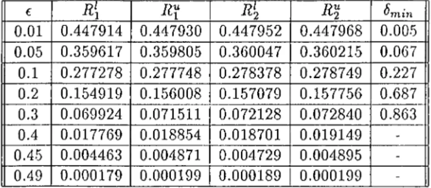
In this section, we present the computational results obtained by using (2.13) for the input constraint given in Figure 1.1 on BSC and ВЕС. The bounds in (2.13) are computed for two different input distributions: first-order and second-order markovian. The parameters are taken as N —7 and T=3. In Tables 2.1 and 2.2, and R\ denote the upper and lower bounds respectively on /¿i, whereas i?2 R2 denote the same bounds for Л2· All bounds are in the unit of nats per channel uses, e denotes the cross-over probability of BSC and the erasure probability for the ВЕС.

We define

CHAPTER 2. CAPACITY OF NOISY, INPUT CONSTRAINED CHANNELS

12

This corresponds to a lower bound on the incremental improvement in percentage gained by using second order markovian distribution on the input sequences of a constrained channel. Tables 2.1 and 2.2 also list the 6ynin values.

The results show that for both channels, when the channel is noisy, the input distri­ bution achieving the capacity is not first-order markovian, since R\ < < R ‘2 < R 2 < C . By considering higher order distributions on the allowed channel input sequences, it seems that further improvements in the maximum rate can be obtained.

We know that for the noiseless channel, first-order markovian distribution achieves capacity. When the channel introduces a low level of noise, i.e., e in BSC and ВЕС is close to zero, 6min is quite small. As the noise level increases, we can gain more in rate by increasing the order. At the extreme point, 6=0.5 in BSC, we know th at the capacity is zero and any probability distribution achieves this rate. Hence, at those values of e near 0.5 we obtain small gains by considering second-order markovian distribution on the channel input sequences. For BSC, higher improvements are obtained for intermediate values of e between 0 and 0.5. Similar comments can be made for constrained ВЕС as e goes to 1.

A situation arising in BSC for e =0.4, 0.45, 0.49 is th at the upper bound on the capac­ ity for the first-order markovian input distribution exceeds the lower bound for the second- order distribution. The same situation occurs also for constrained ВЕС with 6=0.95. This situation is related to the tightness of the bounds. For higher noise levels, knowledge about a particular input letter gives more information about a later channel output let­ ter; thus the entropy of the output letter decreases considerably when conditioned on a previous input letter. The lower bound on the maximum achievable rate by markovian input distribution of constrained BSC is not tight for values of 6 near 0.5 (same situation is valid for ВЕС with 6=1).

This observation may explain the above situation. We can still expect that second- order markovian distribution improves the rate by examining the upper bounds on these values of 6. By increasing the parameter L, it is possible to obtain tighter lower bounds and in this case we can have a more informative answer to this problem.

Another comparison can be made between results of BSC and ВЕС when 6 is between 0 and 0.3. The output of a ВЕС resembles the input more as compared with BSC having a cross-over probability equal to the erasure probability of ВЕС, since observing a non­ erasure letter at the output, we are sure about the corresponding input letter. Therefore, the perturbation on the input sequences of a ВЕС can be thought to be less, compared with BSC having the same cross-over probability. Consequently, optimal one-step distribution achieves rates closer to the capacity for ВЕС. As 6 goes to 0.5, the capacity of constrained BSC approaches zero and improvements become smaller, whereas for constrained ВЕС

CHAPTER 2. CAPACITY OF NOISY, INPUT CONSTRAINED CHANNELS

13

there are improvements for e near 0.5 (capacity of ВЕС goes to zero as c approaches one).

€ _{Ц Ц Щ} ^min 0.01 0.447914 0.447930 0.447952 0.447968 0.005 0.05 0.359617 0.359805 0.360047 0.360215 0.067 0.1 0.277278 0.277748 0.278378 0.278749 0.227 0.2 0.154919 0.156008 0.157079 0.157756 0.687 0.3 0.069924 0.071511 0.072128 0.072840 0.863 0.4 0.017769 0.018854 0.018701 0.019149 -0.45 0.004463 0.004871 0.004729 0.004895 -0.49 0.000179 0.000199 0.000189 0.000199

-Table 2.1: Computed bounds for BSC

€ _Щ R^ _{R ‘2 Щ ^min} 0.01 0.477374 0.477374 0.477375 0.477375 2.10*10-^ 0.05 0.461891 0.461892 0.461915 0.461915 4.98*10-3 0.1 0.442237 0.442238 0.442329 0.442331 0.021 0.2 0.401858 0.401871 0.402206 0.402217 0.083 0.3 0.359922 0.359973 0.360650 0.360668 0.188 0.4 0.316246 0.316380 0.317426 0.317521 0.331 0.5 0.270600 0.270889 0.272244 0.272435 0.500 0.6 0.222699 0.223244 0.224758 0.225081 0.678 0.7 0.172185 0.173100 0.174532 0.175007 0.827 0.8 0.118609 0.119957 0.120990 0.121566 0.861 0.9 0.061426 0.062978 0.063280 0.063925 0.480 0.95 0.031286 0.032542 0.032457 0.032698

-Table 2.2: Computed bounds for ВЕС

2.3

U p p e r b oun d s on C

The upper bounds {Cj\j} on the capacity of BSC and ВЕС with the input constraint given in Fig. 1.1 are tabulated in Tables 2.3 and 2.4. In Tables 2.3 and 2.4, for each channel the upper capacity Cm is provided for the largest value of N th at could be computed. The

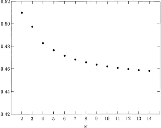
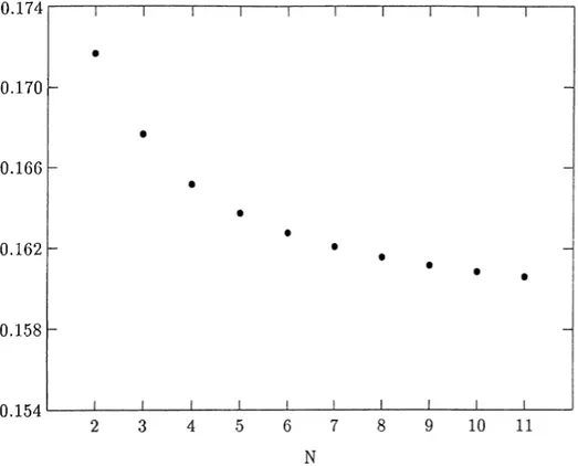
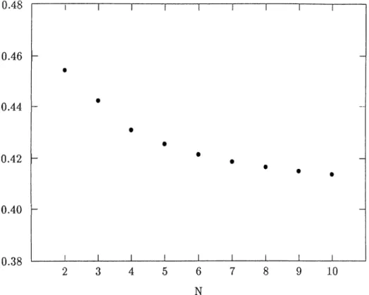
complete list of upper bounds Сдг is given in Appendix B. In Figures (2.1)-(2.6), Cm vs.

N are plotted for various channels considered in this work for giving a visual inspection to the reader.

These values are computed by using Arimoto-Blahut algorithm with an error term 10“ ®. The error term is defined as the difference between results of two consecutive iterations of the algorithm. The number of iterations performed in order to achieve the desired error term are noted.

CHAPTER 2. CAPACITY OF NOISY, INPUT CONSTRAINED CHANNELS

14

The bounds may give some idea about how close markovian distributions on the channel input sequences get to capacity. Obtaining closer bounds by computing C/v for larger values of N was not possible due to extremely long run-times and huge memory requirements.

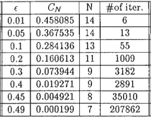
By examining results, one can conclude that assuming markovian distribution on the channel input sequences it is possible to achieve rates near capacity for the channels considered in this work. However, for a more complicated channel the situation may be quite different so that it is possible to achieve considerably much higher rates by using nonmarkovian distributions as compared with the rates achievable by markovian distributions. e Cn N iter. 0.01 0.458085 14 6 0.05 0.367535 14 13 0.1 0.284136 13 55 0.2 0.160613 11 1009 0.3 0.073944 9 3182 0.4 0.019271 9 2891 0.45 0.004921 8 35010 0.49 0.000199 7 207862

Table 2.3: Upper bounds computed by Arimoto-Blahut algorithm(BSC)

6 Cn N # o f iter.

0.1 0.456009 10 8

0.2 0.413863 10 13

0.3 0.370379 10 26

CHAPTER 2. CAPACITY OF NOISY, INPUT CONSTRAINED CHANNELS

15

2.4

R a te o f C on vergen ce o f

C

m

to th e C ap acity

In this section, we will discuss the rate of the convergence Cm to the capacity as N goes to infinity, where

Cm = max

Pn{X^'] N Using (A.5), we can write

N Cm < (A - l)Cyv-i + C i

Rearranging the terms, we obtain

Cm-1 - Cm > Cm- 1 — Cl N

Therefore, the difference between consecutive terms of the sequence {Ca^} goes to zero at fastest reciprocally in A as A goes to infinity. Since we use Arimoto-Blahut algorithm for computing Cyv, which has a computation complexity th at is exponential in A , the rate of convergence of {Cat} is quite small. In Appendix B, we give the complete list of {Cm} computed for the channels considered in this work.

A computationally more efficient way of getting closer to C may be to assume a markovian distribution on the allowed channel input sequences and to find a practical method for computing Rk, By increasing the memory of the input distribution, we can get better estimates of C. The problem is the rate of convergence to Rk as one considers (2.1). We think that the convergence in (2.8) to Rk is achieved exponentially, i.e., the difference between two consecutive terms goes exponentially to zero as A tends to infinity.

As shown in section 2.1, the maximum mutual information of a DMC under input constraints achieved by K-th order stationary markovian distribution can be written in the form (2.8):

Rk = lim rn^x [ H{Y o\ Y- uY-2 ,. . ■ , Y -n) ~ H {Y\ X) ] N-^od

We investigate the difference A a/, between two consecutive terms as we approach the limit in (2.8).

Am = H ( Y o \ Y - u - - - , Y - ( N - i } ) - H{Yo\ Y -u - - - , Y -n) (2.14)

Since conditioning can not increase entropy, Am > 0. Furthermore, convergence in

the capacity assures th at lim Am = 0. We can write (2.14) by using (2.2.26) of [2] in the

N —^oo

form

C H A P T E R 2. C A P A C I T Y OF NOISY, I NPU T C ONS TRAI NE D CHANNELS 16

We can upperbound A^r as

If the rate of convergence in (2.8) is exponential, then A at can be upperbounded with a function which goes to zero exponentially in N as TV —> oo. When the channel output sequences are K-th order markovian, Ayv = 0 for TV > K + 1. However, for an arbitrary distribution on Y ^ , A]\i may be positive for all N. We have proved that when the channel input distribution is ergodic and markovian I(Yo; Y -n) goes to zero exponentially in N as N tends to infinity . There is no general equality or inequality condition between I{Yo]Y~n\ Y-i ) · · · i Y- (N-i)) /(To; Y -n)· However, in our case the sequence Y ^ is not completely arbitrary. The sequences correspond to the output sequences of a DMC when the probability distribution on channel input sequences is markovian. For distributions satisfying the condition that I{Yo\ Y ^m) is larger then /(To; T _ /v |T -i, . . . , y_(yv-i))> the

desired result is shown.

If this statement is true, the upper bound given in (2.13) will be exponentially tight and hence, we can get a good estimate of maximum achievable rate with a markovian distribution on the constrained input sequences. And we can use (2.13) for estimating Rk,

since the convergence will be exponential, we can get close to Rk even for small values of TV. Even the optimal distribution is not markovian in the noisy case, we can still find a good approximation to the capacity by assuming higher order markovian distributions on the channel input sequences.

CHAPTER 2. CAPACITY OF NOISY, INPUT CONSTRAINED CHANNELS

17

0.52 0.50 0.48 0.46 0.44 -0.42 1---1---1---1---1---r "1---1 I--- r I I I I_____\_____ I_____ L

Figure 2.1: Cn v s. N for constrained BSC with c=0.01

0.42 0.40 -0.38 0.36 0 .3 4

-1---- ^

---- r

1---- r

"I--- 1--- ^--- r

•

·

0.32

J _____ L J _____ L J _____ I_____ ^_____ L 2 3 4 5 6 7 8 9 10 11 12 13 14 N

CHAPTER 2. CAPACITY OF NOISY, INPUT CONSTRAINED CHANNELS

18

0.174 0.170 -0.166 0.162 0.158 -0.154

Figure 2.3: Сдг vs. N for constrained BSC with c=0.1

0.52

₁

---

1

---

1

--- г

1

--- г 0.50 0.48 -0.46 0.44

-0.42

J ________I________\________L J _______ I________I________L 2 3 4 5 6 N 7 8 9 10

CHAPTER 2. CAPACITY OF NOISY, INPUT CONSTRAINED CHANNELS

19

0.48 0.46 0.44 0.42 0.40 -0.38

Figure 2.5: Cn vs. N for constrained ВЕС with e=0.2

0.41 0.40 0.39 0.38 0.37

-0.36

_L "I---1---1---1---1--- г J _______ ^________I________L J _______ L 2 3 4 5 6 7 N 8 9 10

C hapter 3

C O N C LU SIO N S

In this work, we v/ere mainly concerned with the capacity of noisy, input-restricted, dis­ crete, memoryless channels. No efficient algorithm is known for computing the capacity of such channels. In particular, we considered BSC and ВЕС with the input restriction given in Fig. 1.1. Our main result is th at, unlike the noiseless case, one-step Markov distribution on the channel input alphabet does not achieve the channel capacity when noise is present. We showed th at a second-order markovian distribution is strictly better than a first order distribution for the BSC and ВЕС with an input constraint in Fig. 1.1.

The amount of incremental improvement in maximum rate by increasing order is also an interesting problem. Code designers search for better codes that achieve higher rates closer to channel capacity. Information about the input distributions on the constrained channel input sequences achieving higher rates is required for finding such codes. Our results show that one may have to use higher order markovian distributions in order to achieve higher rates. However, increasing the order results in an increase in the code complexity. Hence, there is a trade-off between rate and complexity. Future research may be directed at finding bounds on the incremental improvement in the maximum mutual information as one considers higher order markovian distributions on the input sequences of the constrained channel. Such a bound will give an information to the code designer about the trade-off between achievable rate and implementation complexity.

A p p en d ix A

P ro o f th at th e lim it in (1.1) exists

In this part, we present a proof of the existence of the limit in (1.1), i.e., we show that the capacity of a DMC (with an arbitrary input constraint) defined by (1.1) exists.

where C = lim Cat N^oo

^

I{XN-YN)

Cn = max --- —--- ^

Q

n

{X^)

N

and the maximum is taken over the probability distributions on the channel input sequences satisfying channel input constraints. The following is a proof of the limit in (1.1) exists.

Let be the input distribution that achieves Cyv- Let n and / be two positive integers with n + I = N and let X i and X2 be the ensembles of input sequences Xi = ( x i , .. . ,Xn) ^nd X2 = (xni-u · · · â.nd let Yi and Y2 be the resulting channel output ensembles.

N Cn = Iq- J XiX2-,YiY 2 ) ^ Tq^ J XuYi) + TqI,{X2;Yi\ Xi) + Iq^ J XiX2;Y2\Yi) (A .i)

The first term in (A .I) satisfies

/<?· ( X i ; U ) < nCn (A.2)

Since conditional on X i , X2 and Ti are independent, Iq.^{X,;Yi\ Xi) = 0 lQ.^{XiXr,Y2\Yi) = II(Y2\Yi)-iIiY2\XiX2Yi) < I K Y2 ) - n(Y2\X2) = Iq- ^{ Y2; X2)<ICi

21

(A.3) (A.4)

APPENDIX A.

2 2

where the first inequality follows from the fact that unconditioning cannot decrease entropy and conditional on X2 , Y2 is independent of X i and Yi. Combining (A .l), (A.2), (A.3) and (A.4), we obtain

A 6V < nC’n + ICi (A.5)

Applying Lemma 4A.2 of [2, p.ll2 ] for the bounded sequence {Cyv} satisfying (A.o), it follows th a t C exists and is given by

C — lim Cat = infCyv^. N —> 0 0 N

(A.6)

Clearly, > C for all N . Although the sequence {C/v} is not monotonically decreasing, an immediate consequence of (A.5) is

A p p en d ix B

List o f U p per Bounds on th e C apacity

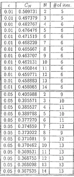
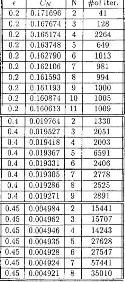
In this appendix, the complete list of upper bounds {Cat} on the capacity of the input- restricted channel, with a constraint represented by the FSM in Fig.1.1. These bounds are computed by using Arimoto- Blahut algorithm.

c Cn N T^of iter. 0.01 0.509731 2 5 0.01 0.497379 3 5 0.01 0.482767 4 6 0.01 0.476476 5 6 0.01 0.471519 6 6 0.01 0.468220 7 6 0.01 0.465667 8 6 0.01 0.463707 9 6 0.01 0.462131 10 6 0.01 0.460844 11 6 0.01 0.459771 12 6 0.01 0.458883 13 6 0.01 0.458085 14 6 0.05 0.405988 2 9 0.05 0.395571 3 10 0.05 0.385527 4 11 0.05 0.389788 5 10 0.05 0.377270 6 11 0.05 0.374859 7 12 0.05 0.373022 8 9 0.05 0.371601 9 12 0.05 0.370462 10 13 0.05 0.369531 11 1 13 0.05 0.368755 12 13 0.05 1 0.368098 13 13 0.05 1 0.367535 14 13

Table B .l: Upper bounds computed by Arimoto-Blahut algorithm(BSC)

APPENDIX B.

24

e _Cn N # o f iter. 0.1 0.310650 2 11 0.1 0.302569 3 21 0.1 0.296059 4 29 0.1 0.292736 5 37 0.1 0.290377 6 43 0.1 0.288729 7 47 0.1 0.287423 8 49 0.1 0.286516 9 51 0.1 0.285743 10 52 0.1 0.285110 11 53 0.1 0.284582 12 54 0.1 0.284136 13 55 0.3 0.077271 2 160 0.3 0.075849 3 691 0.3 0.075173 4 3241 0.3 0.074723 5 2546 0.3 0.074429 6 3029 0.3 0.074222 7 3145 0.3 0.074066 8 3159 0.3 0.073944 9 3182 0.49 0.000200 2 107583 0.49 0.000200 3 150464 0.49 0.000200 4 174862 0.49 0.000200 5 190908 0.49 0.000199 6 201427 0.49 0.000199 7 207862 € Chj N # o f iter. 0.2 0.171696 2 41 0.2 0.167674 3 128 0.2 0.165174 4 2264 0.2 0.163748 5 649 0.2 0.162790 6 1013 0.2 0.162106 7 981 0.2 0.161593 8 994 0.2 0.161193 9 1000 0.2 0.160874 10 1005 0.2 0.160613 11 1009 0.4 0.019764 2 1330 0.4 0.019527 3 2051 0.4 0.019418 4 2003 0.4 0.019367 5 6591 0.4 0.019331 6 2406 0.4 0.019305 7 2778 0.4 0.019286 8 2525 0.4 0.019271 9 2891 0.45 0.004984 2 15441 0.45 0.00-4962 3 15707 0.45 0.004946 4 14243 0.45 0.004935 5 27628 0.45 0.004928 6 27547 0.45 0.004924 7 57441 0.45 0.004921 8 35010 Table B.2: Upper bounds computed by

Arimoto-Blahut algorithm(BSC)

Table B.3: Upper bounds computed by Arimoto-Blahut algorithm(BSC)

APPENDIX B.

25

€ C'n N # o f iter. 0.1 0.502475 2 6 0.1 0.489871 3 7 0.1 0.476003 4 7 0.1 0.469837 5 8 0.1 0.465084 6 8 0.1 0.461885 7 8 0.1 0.459425 8 8 0.1 0.457531 9 8 0.1 0.456009 10 8 0.2 0.454333 2 9 0.2 0.442372 3 10 0.2 0.430993 4 10 0.2 0.425596 5 9 0.2 0.421601 6 9 0.2 0.418860 7 12 0.2 0.416772 8 12 0.2 0.415158 9 12 0.2 0.413863 10 13 0.3 0.404763 2 11 0.3 0.393825 3 15 0.3 0.384691 4 19 0.3 0.380102 5 22 0.3 0.376816 6 24 0.3 0.374529 7 24 0.3 0.372797 8 25 0.3 0.371454 9 26 0.3 0.370379 10 26

R E F E R E N C E S

[1] Shannon, C .E .,“A m athem atical theory of communication,” Bell Syst. Tech. vol.27, pp.379-423(part 1), 1948.

[2] Gallager, R.G., Information Theory and Reliable Communication. New York: Wiley, 1968.

[3] Zehavi, E. and Wolf, J.K .,“On runlength codes,” I T 5^(1988), pp.45-54.

[4] Arimoto, S.,“An algorithm for computing the capacity of arbitrary discrete memoryless channels, ”I T 18 (1972), p p .14-20.

[5] Blahut, R .,“Computation of channel capacity and rate-distortion functions,” IT 18 (1972), pp.460-473.

[6] McEliece, R.J., The theory of information and coding. Massachusetts: Addison-Wesley.