Fractional Fourier optics
Haldun M. Ozaktas
Department of Electrical Engineering, Bilkent University, 06533 Bilkent, Ankara, Turkey
David Mendlovic
Faculty of Engineering, Tel Aviv University, 69978 Tel Aviv, Israel Received May 20, 1994; accepted August 22, 1994
There exists a fractional Fourier-transform relation between the amplitude distributions of light on two spherical surfaces of given radii and separation. The propagation of light can be viewed as a process of continual fractional Fourier transformation. As light propagates, its amplitude distribution evolves through fractional transforms of increasing order. This result allows us to pose the fractional Fourier transform as a tool for analyzing and describing optical systems composed of an arbitrary sequence of thin lenses and sections of free space and to arrive at a general class of fractional Fourier-transforming systems with variable input and output scale factors.
Key words: Diffraction, Fourier optics, optical information processing, fractional Fourier transforms.
1.
INTRODUCTION
The ath-order fractional Fourier transformsFaqˆdsud of the
function ˆqsud is defined for 0 , jaj , 2 as
sFaqˆdsud ;Z
` 2`
Basu, u0d ˆqsu0ddu0,
Basu, u0d ;
expf2isp ˆfy4 2 fy2dg jsin fj1/2
3 expfipsu2cot f 2 2uu0csc f 1 u0 2cot fdg , (1)
where
f;ap
2 (2)
and ˆf sgnssin fd. The kernel is defined separately for a 0 and a 62 as B0su, u0d ; dsu 2 u0d and
B62su, u0d ; dsu 1 u0d, respectively.1,2 One may easily
extend the definition outside the intervalf22, 2g by not-ing that F4j 1aqˆ Faqˆ for any integer j. Both u and u0
are interpreted as dimensionless variables.
Some essential properties of the fractional Fourier transform are as follows: (i) It is linear. (ii) The first-order transform sa 1d corresponds to the com-mon Fourier transform. (iii) It is additive in index, Fa1Fa2qˆ Fa11a2qˆ. Other properties may be found
in Refs. 1 – 11.
Optical implementations of the fractional Fourier transform have already been presented. In Refs. 3 – 7 we discussed the fractional Fourier-transforming property of quadratic graded-index media. Lohmann suggested two systems consisting of thin lenses separated by free space.9
The fact that the two approaches were equivalent and rep-resented the fractional Fourier transform as defined in Refs. 1 and 2 was demonstrated in Ref. 10. Applications have been suggested in these references and in Refs. 7, 11, and 12. Later research13,14 provided certain
exten-sions and experimental verification of the above results.
In this paper we derive a fundamental result stating that there exists a fractional Fourier-transform relation between the (appropriately scaled) optical amplitude dis-tributions on two spherical reference surfaces with given radii and separation (Fig. 1 below). This result provides an alternative statement of the law of propagation and allows us to pose the fractional Fourier transform as a tool for analyzing and describing a rather general class of optical system. (Previous research has been primar-ily concerned with offering optical realization of the frac-tional Fourier transform. These realizations follow as special cases or applications of our more general formula-tion, which allows us to state the necessary and sufficient conditions for a fractional Fourier transform in full gen-erality.)
After discussing in some detail the above-mentioned re-sult, we show how the Fresnel diffraction integral can be expressed in terms of a fractional Fourier transform. We discuss how axially centered systems composed of an arbitrary number of lenses separated by arbitrary dis-tances can be analyzed by means of fractional Fourier transforms. As an instructive example, we concentrate on the classical single-lens imaging configuration. We also specify the general conditions under which an arbi-trary system is a fractional Fourier transformer.
Whenever we can express the result of an optical prob-lem (such as Fraunhofer diffraction) in terms of a Fourier transform, we tend to think of this result as simple and elegant. This is justified by the fact that the Fourier transform has many simple and useful properties that make working with it attractive. The Fourier transform and image occur at certain privileged planes in an opti-cal system. Often all our intuition about what happens in between these planes is that the amplitude distribu-tion is given by a complicated integral. In this paper we show that the distribution of light at intermediate planes can be expressed in terms of the fractional Fourier trans-form (which also has several useful properties and opera-tional formulas). Thus the fractional Fourier transform
completes in a natural way the study of optical systems often called Fourier optics.
We note in passing that, although one-dimensional signals are considered throughout this paper for nota-tional simplicity, straightforward generalization of the results to two dimensions is possible. Although for one-dimensional systems it is more correct to speak of circu-lar (or cylindrical) surfaces, here we customarily speak of spherical surfaces.
As a final word on terminology, we believe that ulti-mately the term Fourier transform should mean, in gen-eral, fractional Fourier transform and that the currently standard Fourier transform should be referred to as the first-order Fourier transform. Likewise, DFT should de-note the discrete (fractional) Fourier transform, etc., and the invention of new acronyms and abbreviations should be discouraged. Then, instead of speaking of fractional Fourier optics, we will be able to speak simply of Fourier optics.
2.
FRACTIONAL
FOURIER-TRANSFORMING PROPERTY OF
PROPAGATION THROUGH FREE SPACE
We refer to Fig. 1. The complex amplitude distribu-tions with respect to the first and the second spherical reference surfaces are denoted by q1sx0d and q2sxd,
re-spectively. The distributions with respect to the planar surfaces tangent to the spherical surfaces on the optical axis are likewise denoted by p1sx0d and p2sxd. If the
radii of the spherical surfaces are denoted by R1and R2,
we have
p2sxd q2sxdexpsipx2ylR2d , (3)
p1sx0d q1sx0dexpsipx0 2ylR1d , (4)
where l is the wavelength. Assuming propagation from left to right, p2sxd is related to p1sx0d by a Fresnel integral:
p2sxd
expsi2pdyldp
ild
Z ` 2`
expfipsx 2 x0d2yldgp
1sx0ddx0.
(5) Combining Eqs. (3) – (5), we can obtain a relation between
q1sx0d and q2sxd. To permit comparison of this relation
with Eq. (1) we introduce the dimensionless variables u0;
x0ys1 and u; xys2, where s1and s2 are real-valued scale
parameters with dimensions of length. Also introducing the hatted functions ˆq1su0d ; q1su0s1d and ˆq2sud ; q2sus2d,
we obtain ˆ q2sud expsi2pdylds1 p ild 3Z ` 2` exp " ip ldsg2s2 2u22 2s 1s2uu01 g1s12u0 2d # 3 ˆq1su0ddu0, (6)
where we established the definitions
g1; 1 1 dyR1, (7)
g2; 1 2 dyR2. (8)
Now, comparing this result with the definition of the fractional Fourier transform [Eq. (1)], we conclude that
ˆ
q2sud is proportional to the fractional Fourier transform
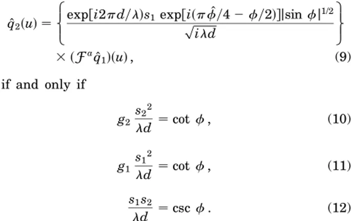
of ˆq1su0d, i.e., ˆ q2sud 8 < :expfi2pdylds
1expfisp ˆfy4 2 fy2dgjsin fj1/2
p ild 9 = ; 3sFaqˆ1dsud , (9) if and only if g2 s22 ld cot f , (10) g1 s12 ld cot f , (11) s1s2 ld csc f . (12) These three equations are the necessary and sufficient conditions for Eq. (9) to hold.
We now discuss the consequences of these equations from three perspectives.
A. Analysis
1. Problem
Given R1, R2, and d, find s1, s2, and a (or, equivalently,
f; apy2). That is, we are given the reference surfaces and wish to find the order and the scale parameters of the resulting transform.
Equations (10) and (11) imply that
g1s12 g2s22. (13)
Now, using the identity cot2f 1 1 csc2f and
Eqs. (10) – (13), we obtain
s24 sldd2s g2yg12 g22d21, (14)
s14 sldd2s g1yg22 g12d21. (15)
Note that Eq. (13) implies that g1g2 $ 0 and that
Eqs. (14) and (15) imply that s g2yg1 2 g22d $ 0 and
s g1yg22 g12d $ 0. These conditions can be summarized
in the form
0 # g1g2# 1 . (16)
If a fractional transform relation is to hold, R1, R2, and
d must be specified such that this condition holds. (It
Fig. 1. Two spherical surfaces. This figure is drawn such that R1 , 0 and R2 . 0. The distance d is always taken to be
is interesting that if Fig. 1 is interpreted as a spherical mirror resonator, this equation is the stability or the confinement condition of the resonator.15)
We can see that, given R1, R2, and d, js2j and js1j
are uniquely determined by Eqs. (14) and (15). Then Eq. (10) or (11) enables us to determine f according to
tan f 6fs1yg1g2d 2 1g1/2, (17)
where the 6 is determined according to the common sign of g1 and g2. The ambiguity in the inverse
tan-gent function is resolved by examination of the sign of csc f. Equation (12) tells us that, if we choose the signs of s1and s2such that s1s2$ 0, then csc f $ 0, so that f
lies inf0, pg. In contrast, if s1s2# 0, then csc f # 0, so
that f lies inf2p, 0g. These results are consistent with inversion and parity properties of the fractional Fourier transform.
2. Result
A fractional Fourier-transform relation exists between two spherical surfaces of radii R1, R2 and separation d
if and only if 0 # g1g2# 1. If this condition is satisfied,
js1j and js2j are determined by Eqs. (14) and (15), and f
is determined within 6p by Eq. (17). The quadrant of f is determined by our choice of the signs of s1 and s2,
or vice versa.
B. Synthesis
1. Problem
Given s1, s2, and a (or, equivalently, f ; apy2), find
R1, R2, and d. That is, we wish to design a fractional
Fourier-transform system with specific order and scale factors.
Notice that Eq. (12) implies that the sign of s1s2 must
be the same as the sign of csc f, which is the same as the sign of f. If s1, s2, and f have been specified consistent
with this requirement, Eq. (12) determines d:
d ss1s2yldsin f . (18)
Then Eqs. (10) and (11) give g1 and g2, which in turn
give R1 and R2:
1 1 dyR1; g1 ss2ys1dcos f , (19)
1 2 dyR2; g2 ss1ys2dcos f . (20)
Note that g1 and g2, as given by these equations, will
always satisfy g1g2 cos2f, and thus 0 # g1g2# 1.
2. Result
A fractional Fourier-transform relation of order a be-tween two spherical surfaces with the input and the out-put scaled by s1 and s2, respectively, can be obtained
if and only if sgnss1s2d sgnssin fd. If this condition
is satisfied, we must choose R1, R2, and d according to
Eqs. (18) – (20).
C. Propagation
1. Problem
Given s1, R1, and d, find a (or f), s2, and R2. That is,
given the radius of the spherical reference surface and
the scale parameter on the input side, find them at a distance d to the right, as well as the order of the resulting transform at that distance.
Because R1and d are given, g1 is also known. Using
Eqs. (10) – (12), we can obtain tan f ld g1s12 , (21) s22 g12s121 sldd 2 s12 , (22) 1 2 dyR2; g2 g1s14 g12s141sldd2 . (23)
We are free to choose the sign of s2, which together with
the specified sign of s1determines the sign of csc f. This
sign determines the quadrant of f in Eq. (21). If we as-sume that s1, s2 are both positive, f lies in the
inter-valf0, pg. Now f, as given by Eq. (21), is a continuous monotonic increasing function of d. Let us assume that the location of the first surface is fixed at the origin z 0 of the optical axis and that we examine the distribution of light after it has propagated a distance z d in the posi-tive z direction. For larger values of d, we observe frac-tional transforms of the initial distribution of larger-order f; the amplitude distribution of light is continuously frac-tional Fourier transformed as it propagates.
2. Result
Given the distribution of light on a spherical reference surface of radius R1 and scale parameter s1, we can
ob-serve its fractional Fourier transform on another spheri-cal reference surface a distance d to the right. The radius
R2 and scale parameter s2 for this surface and the order
of the fractional transform are given by Eqs. (21) – (23), where the quadrant of f is determined by our choice of the sign of s2.
3.
ILLUSTRATIVE APPLICATIONS
We now consider some applications of the above results. For convenience we restrict s1 and s2 to positive values.
This implies csc f . 0, so that f lies in the interval f0, pg. Using Eq. (12) we can now write Eq. (9) in the more meaningful form
ˆ
q2sud fexpsi2pdyldexps2iapy4d
q
s1ys2g sFaqˆ1dsud .
(24) The phase factor expsi2pdyld is associated with propaga-tion over the distance d. The phase factor exps2ify2d is the Gouy phase shift.15 The factorps
1ys2ensures power
conservation.
A. Fresnel Diffraction as a Fractional Fourier Transform
Let us assume that a plane wave of unit amplitude illumi-nates a planar screen with complex amplitude transmit-tance tsxd. We can handle this case by letting R1! `,
as given in Fig. 1. We then have q1sx0d p1sx0d tsx0d.
Because g1 1 in this case, Eq. (11) implies that cot f $
We also assume that the scale parameter s1associated
with the planar reference plane is specified freely. Then Eq. (11) gives us the order of the fractional transform observed at a distance d from the screen. The scale s2
of the transform at this distance can then be found from Eq. (12). Then Eq. (10) yields g2 and hence R2. Thus
the observed field p2sxd at a distance d . 0 is given by
p2sxd fexpsi2pdyldexps2iapy4d p s1ys2gexpfsipx2ylR2dg 3sFaˆtdsxys2d , (25) with ap 2 ; f arctan √ ld s12 ! , (26) s2 s1 " 1 1 sldd 2 s14 #1/2 , (27) R2 d " 1 1 s1 4 sldd2 # , (28)
where ˆtsu0d ; tsu0s
1d. We can eliminate the spherical
phase factor expsipx2ylR
2d by choosing a spherical
ref-erence surface with radius R2, i.e., if we observe g2sxd
instead of p2sxd. (The various phase factors would have
no effect if we were observing only the intensity.) Thus we conclude that the Fresnel diffraction integral can be formulated as a fractional Fourier transform. As
d is increased from 0 to `, the order a of the fractional
transform increases according to Eq. (26) from 0 to 1. Letting d ! `, we obtain the intuitively appealing a 1,
s2 ldys1, and R2 d, which we readily associate with
the Fraunhofer diffraction pattern, which is nothing but the Fourier transform of the diffracting screen.
B. Symmetric Case
Referring to Fig. 1, let us consider the special case in which 2R1 R2 ; R and g1 g2 ; g ; 1 2 dyR.
Equations (10) and (11) then imply that s1 s2, which
we denote by s. The condition 0 # g1g2 # 1 becomes
0 # g2# 1 or, more simply, jgj # 1. This result implies
that 0 # dyR # 2 and hence that R $ dy2. Equations (10) and (12) now become
gss2yldd cot f , (29)
s2yld csc f , (30)
from which it also follows that
g cos f . (31) Given R and d such that jgj # 1, Eq. (31) immediately determines f. Then either Eq. (29) or (30) yields s. Al-ternatively, given f and s, we can use the same equations to find d and g and hence R.
C. Fractional Fourier Transform between Planar Surfaces
We have seen that there exists a fractional Fourier-transform relation between two spherical surfaces, as depicted in Fig. 1. By using a lens to compensate the spherical phase factors at both surfaces, we can obtain a fractional Fourier transform between two planar surfaces.
We simply choose lenses with focal lengths f1 2R1and
f2 R2. Thus, with our synthesis result, it is possible
to design a fractional Fourier transformer of given order
a and of desired input and output scale parameters s1
and s2.
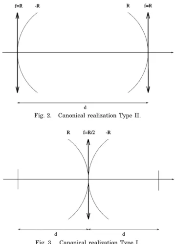
Let us restrict ourselves to the symmetric case for which R $ dy2 . 0. Then, using two positive lenses of focal length f R . 0, we obtain Lohmann’s Type II frac-tional Fourier-transforming system (Fig. 2).9 If the
or-der of the fractional transform apy2 ; f and the scale s are specified, then the separation of the lenses d and their focal length f must be chosen as
d ss2yldsin f , (32)
f ss2yldcotsfy2d. (33)
Alternatively, let us consider an asymmetric pair of spherical surfaces with R1! ` and R2 R. Let us place
immediately to the right of the second surface a thin lens of focal length f Ry2, whose effect will be to map the amplitude distribution on the spherical surface of radius
R onto a spherical surface of radius 2R. Now let us place after the lens a second asymmetric pair of spherical surfaces with R1 2R and R2 ! `. The overall
sys-tem consists of a stretch of free space followed by a lens followed by another stretch of free space, which is noth-ing but Lohmann’s Type I fractional Fourier-transformnoth-ing system (Fig. 3). Its analysis is similar to what has been presented above and is thus not repeated.
We refer to such realizations of the fractional Fourier transform as canonical realizations Type II and Type I.
Fig. 2. Canonical realization Type II.
They are summarized below within the framework of this paper. An alternative discussion of these systems is to be found in Lohmann’s paper.9
Canonical fractional Fourier-transforming configura-tions have planar input and output reference surfaces separated by a distance l and with scale parameter s. The focal lengths of the lenses are denoted by f. The output pout of such a system is related to the input pin
by the relation ˆ
poutsud expsi2plyldexps2iapy4dsFapˆindsud , (34)
where u ; xys2, u0 ; x0ys1 and pˆoutsud ; poutsus2d,
ˆ
pinsu0d ; pinsu0s1d. We can see that the output is
es-sentially the ath-order fractional Fourier transform of the input.
1. Type II
A Type II system consists of a lens of focal length f fol-lowed by a section of free space of length d folfol-lowed by a second lens of focal length f (Fig. 2). Thus its total length is l d. We can obtain d and f in terms of s and f (or a) by using
d ss2yldsin f , (35)
f ss2yldcotsfy2d. (36)
Alternatively, provided that f $ dy2, we can find f (or a) and s in terms of d and f by using
f arccoss1 2 dyfd , (37)
s4 l 2df
2 2 dyf. (38)
2. Type I
A Type I system consists of a section of free space of length
d followed by a lens of focal length f followed by a second
section of free space of length d (Fig. 3). Thus its total length is l 2d. We can obtain d and f in terms of s and f (or a) by using
d ss2yldtansfy2d, (39)
f ss2yldcsc f . (40)
Alternatively, we can find f (or a) and s in terms of d and f by using
f arccoss1 2 dyfd , (41)
s4 l2dfs2 2 dyfd . (42)
D. Classical Single-Lens Imaging
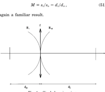
Consider the classical single-lens imaging configuration in which the object is located a distance d0. 0 to the left
of the lens and the image is located a distance di . 0 to
the right of the lens, which has focal length f . 0 (Fig. 4). We can view this system as performing two consecutive fractional Fourier-transform operations (from the object to the lens and from the lens to the image), provided that the radius R2of the spherical reference surface just before the
lens and the radius R1 of the spherical reference surface
just after the lens are related by
1yR1 s1yR2d 2 s1yfd . (43)
This equation states that the amplitude distribution of light on the reference surface with radius R2 is mapped
by the lens onto a reference surface with radius R1. If we
are to look into the combined effect of the two consecutive fractional transforms, we should choose the scale factors
s2 and s1 immediately before and immediately after the
lens such that
s1 s2. (44)
Letting fo; aopy2 and fi; aipy2 denote the order of
transformation occurring from the object to the lens and from the lens to the image, respectively, we can write the imaging condition (for an inverted image) as ao1 ai 62
or, equivalently,
fo1 fi 6p . (45)
This condition follows from the fact that F62f ˆqsudg
ˆ
qs2ud for any ˆqsud.
Now, with the definitions g2 ; 1 2 doyR2, g1 ; 1 1
diyR1, we have [see Eqs. (10) and (11)]
cot fo g2ss22yldod , (46)
cot fi g1ss12yldid . (47)
It is now possible to show that Eq. (45) implies the well-known imaging condition
1yf s1ydod 1 s1ydid . (48)
Furthermore, if we let soand si denote the scale factors
associated with the object and the image, Eq. (12) lets us write
sos2yldo csc fo, (49)
s1siyldi csc fi. (50)
Now, because Eq. (45) implies that csc fo csc fi, we
obtain the magnification M of the scale factors
M; siyso diydo, (51)
again a familiar result.
E. General Lens Systems Analyzed as Consecutive Fractional Fourier Transforms
More-complicated systems involving several lenses sepa-rated by arbitrary distances can be analyzed in a similar manner. For simplicity let us restrict ourselves to posi-tive lenses. Let the distance separating the input (or the object) from the first lens be d0; the distance separating
the first and the second lens, d1; and the distance
sepa-rating the ith and thesi 1 1dth lens, di. The focal length
of the ith lens is denoted by fi. In general, the subscripts
i2 and i1 are used to denote quantities immediately to
the left and the right of the ith lens, respectively. fi
de-notes the order of the fractional transform associated with propagation from lens i to lens i 1 1.
Assume that the input is specified with respect to a particular spherical reference surface of radius R01 and
that the input scale parameter is denoted by s01. Just
before the first lens in the system we observe the frac-tional Fourier transform of the input of order f0, where
f0can be calculated from cot f0 g01s012yld0[Eq. (11)],
with g01 ; 1 1 d0yR01. The scale of this transform is
s12 sld0ys01dcsc f0[Eq. (12)], and the transform is
ob-served on a spherical reference surface of radius R12,
which we can calculate from g12; 1 2 d0yR12and g12
sld0ys122dcot f0 [Eq. (10)].
Now we can make our way through the lens, using
s11 s12 and 1yR11 1yR122 1yf1[Eqs. (43) and (44)].
Then, just before the second lens, on a spherical reference surface of radius R22, we observe the fractional Fourier
transform of the input of order f01 f1, and so on.
Let us assume that all d0, d1, . . . , f1, f2, . . ., as well
as s01 and R01, are specified. Then we can work our
way through the system iteratively, using the following equations for i 0, 1, 2, . . . :
gi1 1 1 diyRi1, (52)
cot fi gi1si12yldi, (53)
ssi11d2 sldiysi1dcsc fi, (54)
ssi11d1 ssi11d2, (55)
gsi11d2 fldiyssi11d22gcot fi, (56)
Rsi11d2 di
1 2 gsi11d2
, (57)
Rsi11d1ffi11Rsi11d2
i112 Rsi11d2
. (58)
Here si1 and Ri1 may be considered to be the state
vari-ables of the iteration. The cumulative order of the trans-form just before the ith lens is fcumi f01 f11 · · · 1
fi21. This procedure allows us to find the orders of the
transforms at the lenses, but of course it is also possible to calculate the order of the transform observed at any intermediate location (the propagation result).
Thus we can see that, in an optical system involving many lenses separated by arbitrary distances, the ampli-tude distribution is continuously fractional Fourier trans-formed as it propagates through the system. The order fszd of the fractional transform observed at the distance
z along the optical axis is a monotonically increasing
function. The transforms are observed on spherical
ref-erence surfaces. Wherever the order of the transform fszd is equal to s4j 1 1dpy2 for any integer j, we observe the Fourier transform of the input. Wherever the order is equal tos4j 1 2dpy2, we observe an inverted image, etc. The results of this subsection can be generalized for systems composed of an arbitrary sequence of spherical refracting surfaces.
F. Interpretation of Quadratic Graded-Index Media as a Continuum of Infinitesimal Thin Lenses Interspersed with Infinitesimal Sections of Free Space
The fractional Fourier-transforming property of quadratic graded-index media was discussed in Refs. 4 – 7 and 10. The refractive index in such a medium has the following dependence on x:
n2sxd n02f1 2 sxyjd2g , (59)
where n0 . 0 and j . 0 are the medium parameters.
In considering such a medium of length l, the output is related to the input by Eq. (34) just as well, provided that we replace l ! lyn0. Now f; apy2 and s . 0 are given
in terms of n0, j, and l by
f lyj , (60)
s2 ljyn
0. (61)
Now we discuss the relation between such fractional Fourier transformers and the canonical systems discussed in Subsection 3.C. Let us consider Type I (the discussion is similar for Type II). Assume that we cascade N Type I systems, each of length 2d, so that the overall length of the system is l N2d. Now, keeping this overall length and the scale parameter s fixed, we let N ! ` and 2d ! 0. Physically, what we obtain is a large number of closely spaced weak-focal-power lenses.16 In the limit
the average refractive-index distribution of this assembly will have a quadratic dependence on x, similar to Eq. (59). To see that this is true, let us consider optical paths parallel to the optical axis. Using small f approxima-tions of Eqs. (39) and (40), we can show that the phase collected along such a path through the infinite cascade of infinitesimal Type I systems is
.2pfsxysd2
, (62)
where we have dropped the constant term 2pN2dyl. Turning our attention to quadratic index media, Eqs. (59) – (61) allow us to write the collected phase in exactly the same form as above. This means that if we assume functional equivalence of the two sys-tems (identical values of f and s) we can deduce their physical equivalence (identical collected phase, which is proportional to optical density).
From the same sets of equations we can derive another relation that is valid for both cases:
f slys2d, , (63)
4.
GENERAL CONDITIONS FOR
THE OPTICAL FRACTIONAL
FOURIER TRANSFORM
The class of quadratic-phase systems17–21is characterized
by linear transformations of the form
poutsxd Z` 2` hsx, x0dpinsx0ddx0, hsx, x0d C expfipsax22 2bxx0 1 gx0 2dg , (64) where C is a complex constant, and a, b, and g are real constants independent of x and x0. Optical systems
in-volving an arbitrary sequence of thin lenses and sections of free space (in the Fresnel approximation) belong to this class. (We can easily show this by first proving that the kernel for a section of free space followed by a lens and a lens followed by a section of free space both assume the above form and by then noting that an arbitrary system can be composed of these units.)
For this class of systems it is sufficient to specify the pa-rameters C, a, b, and g to characterize the system com-pletely. The condition for a fractional Fourier transform can be stated in terms of these parameters as follows. There should exist scale parameters s1, s2such that
as22 cot f gs12, (65)
bs1s2 csc f (66)
for some f. It can be shown that such scale parameters can be found if and only if 0 # ag # b2. If this condition
is satisfied, the necessary scale parameters and the order of the resulting transform are given by
s14 s b2gya 2 g2d21, (67)
s24 s b2ayg 2 a2d21, (68)
tan f 6s b2yag 2 1d1/2, (69) where the sign of tan f is the same as the identical signs of a and g and where f lies in the intervalf2p, 0g or f0, pg according to whether bs1s2# 0 or bs1s2$ 0. For
example, if s1s2 $ 0, a $ 0, and b $ 0, f lies in the
interval f0, py2g.
If the condition 0 # ag # b2 is not satisfied, it is still
possible to observe a fractional Fourier transform between spherical (rather than planar) reference surfaces at the input and the output. (That is, it is possible to take any system and make a fractional Fourier transformer out of it by appending lenses to the input and the output.) To show this, we note that the kernel h0sx, x0d between
the new spherical reference surfaces will be modified ac-cording to a0 a 2 1ylR
2, b0 b, and g0 g 1 1ylR1,
where R1and R2are the radii of the new input and
out-put reference surfaces. Now we can always ensure that 0 # a0g0# b0 2by an appropriate choice of R
1and R2.
It is possible to arrive at the same results through a different formalism. Let us define the transformation matrix characterizing the optical system as
" A C B D # ; " gyb 2b 1 agyb 1yb ayb # " ayb b 2 agyb 21yb gyb #21 , (70)
with determinant AD 2 BC 1. There are many rea-sons for defining such a matrix. First, if several systems, each characterized by such a matrix, are cascaded, one can find the matrix characterizing the overall system by mul-tiplying the matrices of the several systems. Second, the effect of the optical system on the Wigner distribution17,18
of the input is easily expressed in terms of this matrix. Third, this matrix can be made the basis of a geometrical-optics description of a quadratic-phase system; it is es-sentially the well-known ray matrix.15 These issues are
discussed extensively in the research of Bastiaans,17–21so
they are not considered further here. (Bastiaans actu-ally deals with the inverse of the above matrix.)
Introducing the variables u; xys2 and u0 ; x0ys1 in
Eqs. (64), one can write the kernel as / expfipsau2
2 2buu01 gu0 2dg, with a as
22, b bs1s2, and g gs12.
It is now possible to show that the elements of the new transformation matrix associated with the dimensionless variables are related to the elements of the original trans-formation matrix given in Eq. (70):
2 4 A C B D 3 5 " gyb 2b 1 a gyb 1yb ayb # " As1ys2 Cs1s2 Bys1s2 Ds2ys1 # . (71)
The transformation matrix associated with the frac-tional Fourier transform of order f is the rotation matrix4,9,10 " cos f 2sin f sin f cos f # . (72)
Thus the condition for a fractional Fourier transform is that there exist scale parameters s1and s2such that the
matrices given in expressions (71) and (72) are equal for some f. The necessary and sufficient condition for such scale parameters to exist can be expressed as 0 # AD # 1 (or, equivalently, 21 # BC # 0). If this condition is satis-fied, the necessary scale parameters and the order of the resulting transform are given by
s14 B2sAyD 2 A2d21, (73)
s24 B2sDyA 2 D2d21, (74)
cos f 6sADd1/2, (75)
where sgnscos fd sgnsAs1ys2d and f lies in the
inter-valf2p, 0g or f0, pg according to whether Bys1s2# 0 or
Bys1s2$ 0. For example, if s1s2$ 0, A $ 0, and B $ 0,
f lies in the interval f0, py2g.
If the condition 0 # AD # 1 is not satisfied, we can still make a fractional Fourier transformer out of this sys-tem by appending lenses at its input and output surfaces. (That is, for any system, it is possible to find spherical in-put and outin-put reference surfaces between which a frac-tional Fourier-transform relation exists.) To show this, we multiply the transformation matrix from the left and the right by the transformation matrix of a thin lens15:
" A0 C0 B0 D0 # " 1 2K2 0 1 #" A C B D #" 1 2K1 0 1 # , (76)
where K1, K2 are measures of the powers of the lenses.
Multiplying the matrices, we find that A0 A 2 K 1B
and D0 D 2 K
2B. It is clearly possible to satisfy the
condition 0 # A0D0
# 1 by an appropriate choice of K1
and K2.
5.
CONCLUSIONS
There exists a fractional Fourier-transform relation be-tween two spherical reference surfaces of given radii and separation. It is possible to determine the order and the scale parameters associated with this fractional trans-form, given the radii and the separation of the surfaces. Alternatively, given the desired order and scale parame-ters, it is possible to determine the necessary radii and separation.
The propagation of light along the 1z direction can be viewed as a process of continual fractional Fourier trans-formation. As light propagates, its distribution evolves through fractional transforms of increasing orders. The order fszd of the fractional transform observed at z is a continuous monotonic increasing function of z. (The fractional transform at z is observed on a spherical refer-ence surface intersecting the optical axis at that location.) One of the central results of diffraction theory is that the far-field diffraction pattern is the Fourier transform of the diffracting object. Thus we have shown that the field at a closer distance is the fractional Fourier transform of the diffracting object.
The effect of a thin lens on such a propagating wave-form is merely to bend the spherical reference surface into another reference surface with a different radius. Thus we can continue tracking the evolution of the wave in terms of fractional Fourier transforms, starting from this new reference surface.
It has been shown by Onural22 that the propagation
of light in the Fresnel approximation can be viewed as a wavelet transform. The relation between fractional Fourier transforms and wavelet transforms is discussed in Ref. 7, so that Onural’s result can be tied to ours.
We have discussed rather carefully what we have termed canonical fractional Fourier-transforming sys-tems, which are the simplest symmetric configurations yielding a fractional Fourier transform between pla-nar reference surfaces. We also showed that quadratic graded-index media can be viewed as the limit of a larger and larger number of weaker and weaker lenses.
We derived the (well-known) single-lens imaging equa-tions, starting from an imaging condition stated in terms of fractional Fourier transforms. Generalizing, we saw that fractional Fourier transforms provide a new way of analyzing optical systems involving several lenses sepa-rated by arbitrary distances. Such systems can be an-alyzed by means of geometrical optics, Fresnel integrals (spherical-wave expansions), plane-wave expansions, Hermite – Gaussian beam expansions, and, as we showed, fractional Fourier transforms. The various approaches prove useful in different situations and provide differ-ent viewpoints that complemdiffer-ent each other. The frac-tional Fourier-transform approach is appealing in that it describes the continuous evolution of the wave as it propagates through the system.
Finally, we considered a rather general class of optical
systems and stated the general conditions that a member of this class must satisfy for its output to be viewed as the fractional Fourier transform of its input. We also showed that one can make a fractional Fourier transformer out of any system by appending lenses of appropriate focal length at the input and the output faces.
It is also of interest to formulate our results in the framework and the conventions of Hermite – Gaussian beams. This approach is suitable for studying beam propagation and spherical mirror resonators.14
We have avoided discussing complex-order transforms so as to avoid dealing with complex-valued scale param-eters s1and s2. Such systems do not satisfy 0 # g1g2#
1. Thus, if Fig. 1 is interpreted as a spherical mirror resonator, we are dealing with an unstable resonator.14
This case might be worth investigating.
ACKNOWLEDGMENT
It is a pleasure to acknowledge the contributions of Adolf W. Lohmann of the University of Erlangen-N ¨urnberg, which were made in the form of many discussions and suggestions. He has been a constant source of inspira-tion throughout this research.
Note added in proof: The reader is also referred to Refs. 23 and 24, two recent publications that discuss similar results.
REFERENCES AND NOTES
1. V. Namias, “The fractional Fourier transform and its appli-cation in quantum mechanics,” J. Inst. Math. Its Appl. 25, 241 – 265 (1980).
2. A. C. McBride and F. H. Kerr, “On Namias’s fractional Fourier transform,” IMA J. Appl. Math. 39, 159 – 175 (1987). 3. D. Mendlovic, H. M. Ozaktas, and A. W. Lohmann, “Fourier transforms of fractional order and their optical interpreta-tion,” in Optical Computing, Vol. 7 of 1993 OSA Technical Digest Series (Optical Society of America, Washington, D.C., 1993), pp. 127 – 130.
4. H. M. Ozaktas and D. Mendlovic, “Fourier transforms of frac-tional order and their optical interpretation,” Opt. Commun.
101, 163 – 169 (1993).
5. D. Mendlovic and H. M. Ozaktas, “Fractional Fourier trans-formations and their optical implementation. I,” J. Opt. Soc. Am. A 10, 1875 – 1881 (1993).
6. H. M. Ozaktas and D. Mendlovic, “Fractional Fourier trans-forms and their optical implementation. II,” J. Opt. Soc. Am. A 10, 2522 – 2531 (1993).
7. H. M. Ozaktas, B. Barshan, D. Mendlovic, and L. Onural, “Convolution, filtering, and multiplexing in fractional Fourier domains and their relation to chirp and wavelet transforms,” J. Opt. Soc. Am. A 11, 547 – 559 (1994). 8. L. B. Almeida, “The fractional Fourier transform and
time-frequency representations,” IEEE Trans. Signal Process. 42, 3084 (1994).
9. A. W. Lohmann, “Image rotation, Wigner rotation, and the fractional Fourier transform,” J. Opt. Soc. Am. A 10, 2181 – 2186 (1993).
10. D. Mendlovic, H. M. Ozaktas, and A. W. Lohmann, “Graded-index fibers, Wigner-distribution functions, and the frac-tional Fourier transform,” Appl. Opt. 33, 6188 – 6193 (1994). 11. A. W. Lohmann and B. H. Soffer, “Relationship between two transforms: Radon – Wigner and fractional Fourier,” in An-nual Meeting, Vol. 16 of 1993 OSA Technical Digest Series (Optical Society of America, Washington, D.C., 1993), p. 109. 12. D. Mendlovic, H. M. Ozaktas, and A. W. Lohmann, “Self Fourier functions and fractional Fourier transforms,” Opt. Commun. 105, 36 – 38 (1994).
13. R. G. Dorsch, A. W. Lohmann, Y. Bitran, D. Mendlovic, and H. M. Ozaktas, “Chirp filtering in the fractional Fourier domain,” Appl. Opt. 11, 7599 – 7602 (1994).
14. H. M. Ozaktas and D. Mendlovic, “Fractional Fourier trans-form as a tool for analyzing beam propagation and spherical mirror resonators,” Opt. Lett. 19, 1678 – 1680.
15. B. E. A. Saleh and M. C. Teich, Fundamentals of Photonics (Wiley, New York, 1991).
16. A similar limiting process is discussed in P. J. Readon and R. A. Chipman, “Maximum power of refractive lenses: a fundamental limit,” Opt. Lett. 15, 1409 – 1411 (1990). 17. M. J. Bastiaans, “The Wigner distribution applied to optical
signals and systems,” Opt. Commun. 25, 26 – 30 (1978). 18. M. J. Bastiaans, “Wigner distribution function and its
application to first-order optics,” J. Opt. Soc. Am. A 69, 1710 – 1716 (1979).
19. M. J. Bastiaans, “The Wigner distribution function and Hamilton’s characteristics of a geometric-optical system,” Opt. Commun. 30, 321 – 326 (1979).
20. M. J. Bastiaans, “Propagation laws for the second-order mo-ments of the Wigner distribution function in first-order op-tical systems,” Optik 82, 173 – 181 (1989).
21. M. J. Bastiaans, “Second-order moments of the Wigner dis-tribution function in first-order optical systems,” Optik 88, 163 – 168 (1991).
22. L. Onural, “Diffraction from a wavelet point of view,” Opt. Lett. 18, 846 – 848 (1993).
23. P. Pellat-Finet, “Fresnel diffraction and the fractional-order Fourier transform,” Opt. Lett. 19, 1388 – 1390 (1994). 24. P. Pellat-Finet and G. Bonnet, “Fractional order Fourier
transform and Fourier optics,” Opt. Commun. 111, 141 – 154 (1994).